Article

Application of Machine Learning in Forecasting the Impact of Mining Deformation: A Case Study of Underground Copper Mines in Poland

by
Konrad Cieślik
1,* and
Wojciech Milczarek
2
1
TrainAI GmbH, Oberhusrain 12, 6010 Kriens, Switzerland
2
Department of Geodesy and Geoinformatics, Faculty of Geoengineering Mining and Geology, Wroclaw University of Science and Technology, Wybrzeże Wyspiańskiego 27, 50-370 Wrocław, Poland
*
Author to whom correspondence should be addressed.
Remote Sens. 2022, 14(19), 4755; https://doi.org/10.3390/rs14194755
Submission received: 2 August 2022 / Revised: 14 September 2022 / Accepted: 16 September 2022 / Published: 23 September 2022

Abstract

:
Open access to SAR data from the Sentinel 1 missions allows analyses of long-term ground surface changes. The current data-acquisition frequency of 12 days facilitates the continuous monitoring of phenomena such as volcanic and tectonic activity or mining-related deformations. SAR data are increasingly also used as input data in forecasting phenomena on the basis of machine learning. This article presents the possibility of using selected machine learning algorithms in forecasting the influence of underground mining activity on the ground surface. The study was performed for a mining protective area with a surface of over 500 km 2 and located in western Poland. The ground surface displacements were calculated for the period from November 2014 to July 2021, with the use of the Small Baseline Subset (SBAS) method. The forecasts were performed for a total of 22 identified subsidence troughs. Each of the troughs was provided with two profiles, with a total of more than 10,000 identified points. The selected algorithms served to prepare 180-day displacement forecasts. The best results (significantly better than the baseline) were obtained with the ARIMA and Holt models. Linear models also provided better results than the baseline and their performance was very good at up to 2 months forecasting. Tree-based models including their sophisticated ensemble versions: bagging (Random Forest, Extra Trees) and boosting (XGBoost, LightGBM, CatBoost, Gradient Boosting, Hist Gradient Boosting) cannot be used for this type of predictions since Decision Trees are not able to extrapolate and thus are not a valid stand-alone tool for forecasting in this type of problems. A combination of satellite remote sensing data and machine learning facilitated both the simultaneous quasi-permanent monitoring of ground surface displacements and their forecasting in a relatively long time period.

1. Introduction

Global challenges faced by humans require an increasingly broader and more rapid access among other things to high-quality remote sensing satellite data. Earth observations (EO) and technologies based on research performed from space already play a significant role in generating relevant sets of information which support generally understood disaster management strategies [1,2,3]. A combination of the data currently obtained from space with long series data collected for more than thirty years means that ground surface changes can be traced across the entire planet. A natural application direction for the unprecedented amounts of EO data is to employ them in forecasting future phenomena on the basis of machine learning algorithms. Such forecasts can be performed on a regional [4,5], as well as on a local scale [6,7,8].
Mining-induced ground surface deformations represent a negative result of human activity on the local scale. Ground surface displacements due to mining activity are observed regardless of the mining method (underground, surface or borehole). In many regions of the world, long-term mining exploitation caused a discontinuous [9] and/or continuous [10] degradation of the ground surface. The impact of mining operations is most often manifested on the surface in the form of continuous subsidence troughs which directly result from the formation of empty spaces in the rock mass. These manifestations occur across a lengthy period of time and may depend on a number of factors, such as the mining method (the mining system and depth), or the geological and hydrogeological conditions. Such surface displacements may be experienced even many years after the mining operation is discontinued [11].
Synthetic aperture radar interferometry (InSAR) facilitates the monitoring of the ground surface in order to detect and trace changes of altitude which result from phenomena such as volcanic patterns [12,13], tectonics [14], mining [15], landslides [8], oil and gas extraction [16], pumping water from underground reservoirs [17] or floods [18], as well as glacier displacement [19]. The potential of InSAR methods is demonstrated by the ability to simultaneously trace/monitor changes of ground surfaces with an area of approx. 48,000 km 2 (in the case of Sentinel 1A/1B satellites) with an interval of 10–15 days (due to the SAR data acquisition time). The research results to date demonstrate that InSAR can be successfully used in long-term analyses of surface displacement in mining [20] and post-mining [21,22] areas.
The ability to forecast and estimate the scale of such displacements is an important issue from the perspective of protecting mining areas and minimizing the impact of mining activity on the surface. A number of methods have been developed for forecasting mining-induced surface displacements. They include inter alia empirical methods (the Budryk–Knothe method) and numerical methods (finite element method, discrete element method). Recent years have witnessed the rapid development and increasingly intensive application of machine learning methods, which are based on a broad range of mathematical and statistical methods for building models, and which can be trained on the basis of prepared training datasets. Subsequently, using the relationships present in the training data, machine learning models can forecast the result for the new test data provided to the model.
Machine learning algorithms require large sets of labeled data to train the predictive model. Such data may be provided by synthetic aperture radar interferometry which, unlike GNSS for example, facilitates the detection of ground surface displacements with a significantly higher spatial density. The development of machine learning methods has been accompanied by publications linking them to InSAR measurements [23,24]. However, the number of publications describing solutions related to mining-induced deformations is still limited.
This article analyzes ground surface displacements in the mining protective area of the Legnica-Głogów Copper Belt (LGCB), where 22 subsidence troughs were identified. The ground surface displacements were identified on the basis of satellite radar data from the Sentinel 1 constellation. Long-term displacements were calculated with the use of the Small Baseline Subset (SBAS) method. Using the SBAS results, an attempt was made to forecast deformations based on the identified Line of Sight (LOS) displacements and on selected machine learning algorithms. The machine learning models were assumed to be capable of learning with historical InSAR data and of predicting unseen data—of forecasting future elevation changes. This can provide important insights about the environmental impact of mining operations or natural processes.
The main objective of the study was to determine the forecast displacement values within the limits of all active subsidence troughs in the LGCB area and to evaluate the accuracy of the obtained results. In this article, only the results of ground surface displacement based on the SBAS method were used to build machine learning models and to validate the results afterward. The results obtained are satisfactory. In further studies, once additional geomechanical data are available, the data will be included as training data for new models.

2. Area of Interest

The Legnica-Głogów Copper Belt (LGCB) is located in the area of the Fore Sudetic monocline, in South-West Poland (Figure 1). The area is rich in copper ore, which is currently mined from six deposits by the following three mining plants: Lubin, Rudna and Polkowice-Sieroszowice. The area of the KGHM Polska Miedź S.A. deposit extends 40 km in the strike direction and 20 km in the dip direction, and its depth is from 370 to 1380 m. The copper ore deposit in this area is a sediment-hosted stratabound deposit of the Zechstein copper shales. The deposit is located mainly in the floor part of the Zechstein formation and in the roof part of the Rotliegend sediments. The copper ore deposit is composed of copper sulfide present in white and white-gray sandstone from Rotliegend and Zechstein, as well as in copper shales and Zechstein carbonate rocks. The mined deposit is one of the largest polymetallic deposits in the world. Its area exceeds 750 km 2 . Copper ore in the LGCB region is generally formed in the following three types of rocks: Rotliegend and Grauliegend sandstones, Zechstein copper shales and carbonate rocks. Rocks of the last type, which are typically found in the roofs of the excavations, show high levels of strength and the ability to accumulate elastic energy; therefore, they facilitate the occurrence of tremors [25].
The mining operations are performed following the retreat mining method in the room and pillar system with hydraulic backfill (in the case of areas requiring surface protection). In the case of the LGCB, the extent of continuous ground surface deformations is consistent with the range of a particular deposit within an area of the copper belt. The scale of deformations is mostly influenced by the thickness of the mined rock mass and by the method applied to the liquidation of the mined-out areas. The first and dominating type of deformations are direct continuous deformations represented by land surface deformations manifested as ground subsidences (subsidence troughs) whose range extends beyond the contour of the mining operation. Deformations of the second type result from paraseismic activity. Prior works concerning ground surface deformation analysis for the LGCB area have shown that for most of the identified subsidence troughs, the observed displacements are characterized by long-term linear trends [20,26].

3. Materials and Methods

Long-term displacements were identified on the basis of data from descending orbit no. 73, Figure 1. The LOS displacement calculations were performed with the use of the SBAS method [27] and with simultaneous allowance for the method of reducing the influence of the atmosphere [28]. The temporal base for the presented research was almost 7 years, from November 2014 until July 2021. Based on previous studies for this area, the spatial and temporal base was assumed as standard, at 50 m and 50 days (Table 1). A total of 295 SAR images served to calculate more than 1300 interferograms.
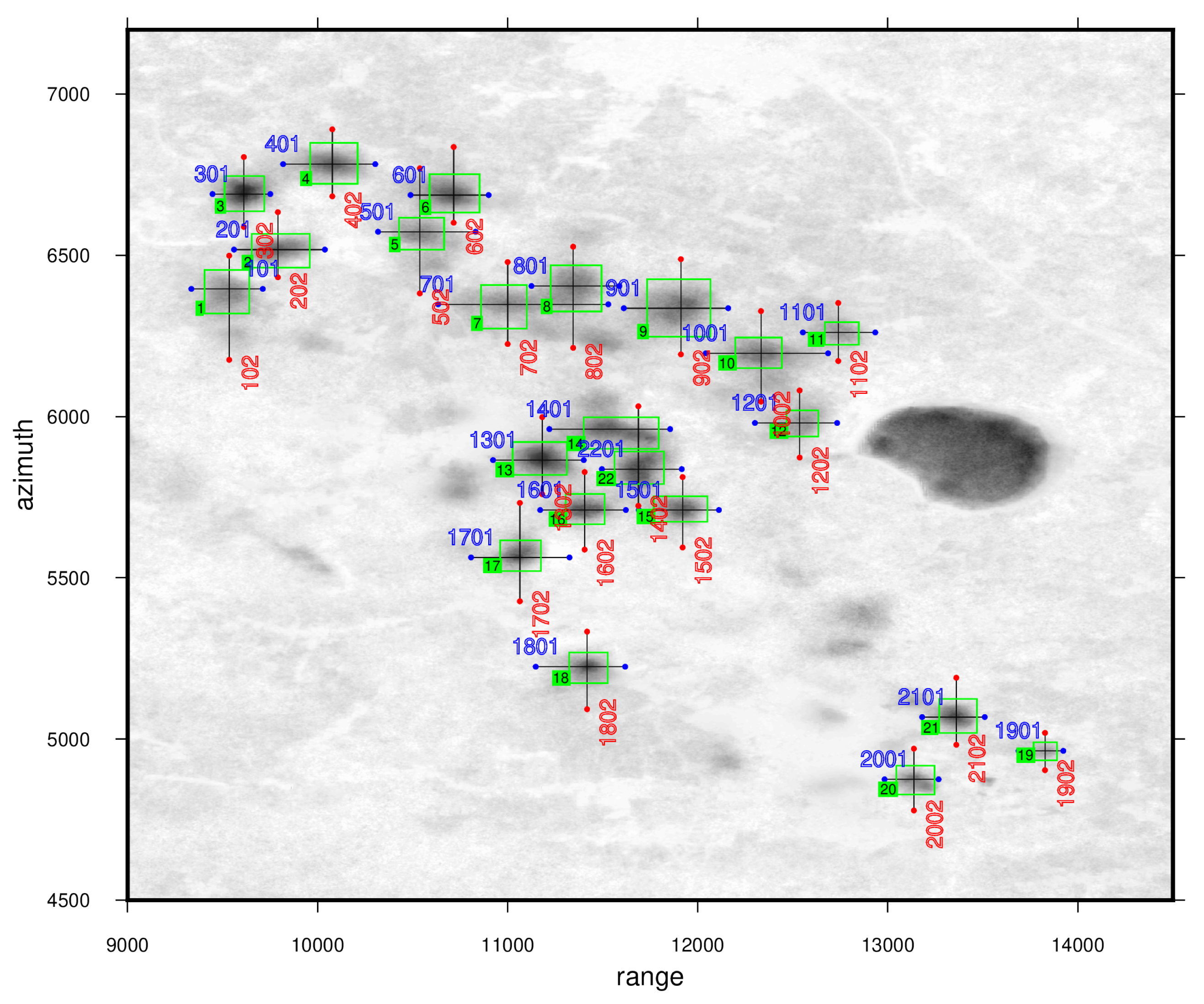
The values of ground surface displacement were forecasted for points located on selected profiles. All of the 22 identified subsidence troughs have two such profiles (Figure 2). One of the profiles is in the azimuth direction, and the other profile is in the range direction (the satellite system). A total of 10,261 points were identified for all of the profiles.
The application of machine learning algorithms in forecasting ground surface displacement in mining areas based on an InSAR time series is a relatively new object of research. Table 2 contains examples of using selected algorithms in analyzing satellite radar data.
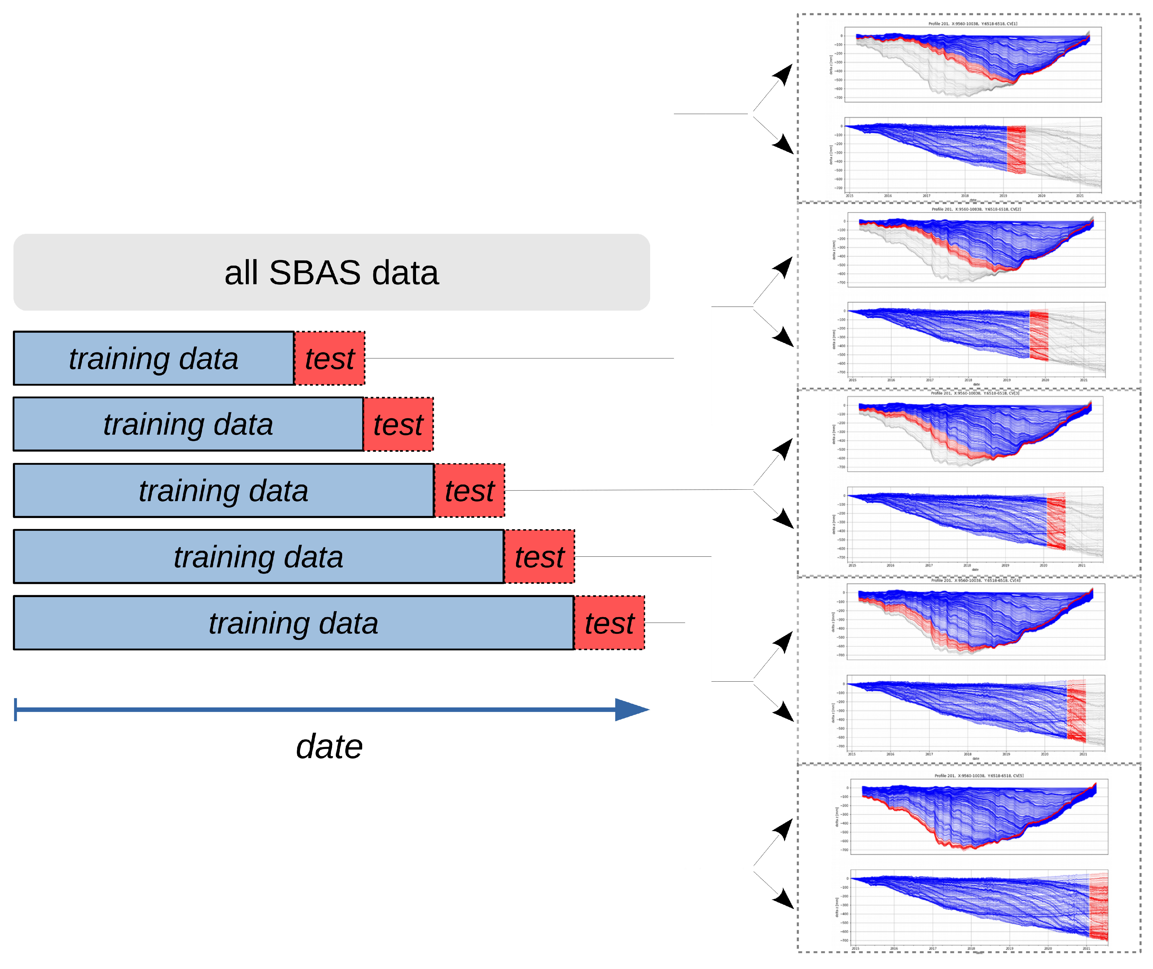
The range of data used in this analysis covers data collected between 15 November 2014 and 23 July 2021. With a regular sampling rate of 6 days, this resulted in 408 samples per location. Any gaps in the data were filled with linear interpolation. Then the data were split into five cross validation (CV) groups (Figure 3, Table 3) using the time-series split approach (ref: scikit-learn.org, accessed on 22 June 2022) with a fixed test size of 30 samples which corresponds to 180 days of the forecasting horizon.
It must be noted that inside all CV test subsets, there were only three dates with missing data (2% of the entire CV dataset). The size of the training dataset is initially 258 samples for the first CV group and increases by 30 samples for each subsequent group to finally reach 378 samples for the fifth and last CV group.
This study focuses mainly on machine learning (ML) models used for forecasting and does not test any deep learning (DL) models. In similar studies, DL models did not provide good results and performed even worse than naive approaches so they were excluded from the analysis. As discussed in the results section, most ML forecasting methods performed significantly better than the naive approaches.
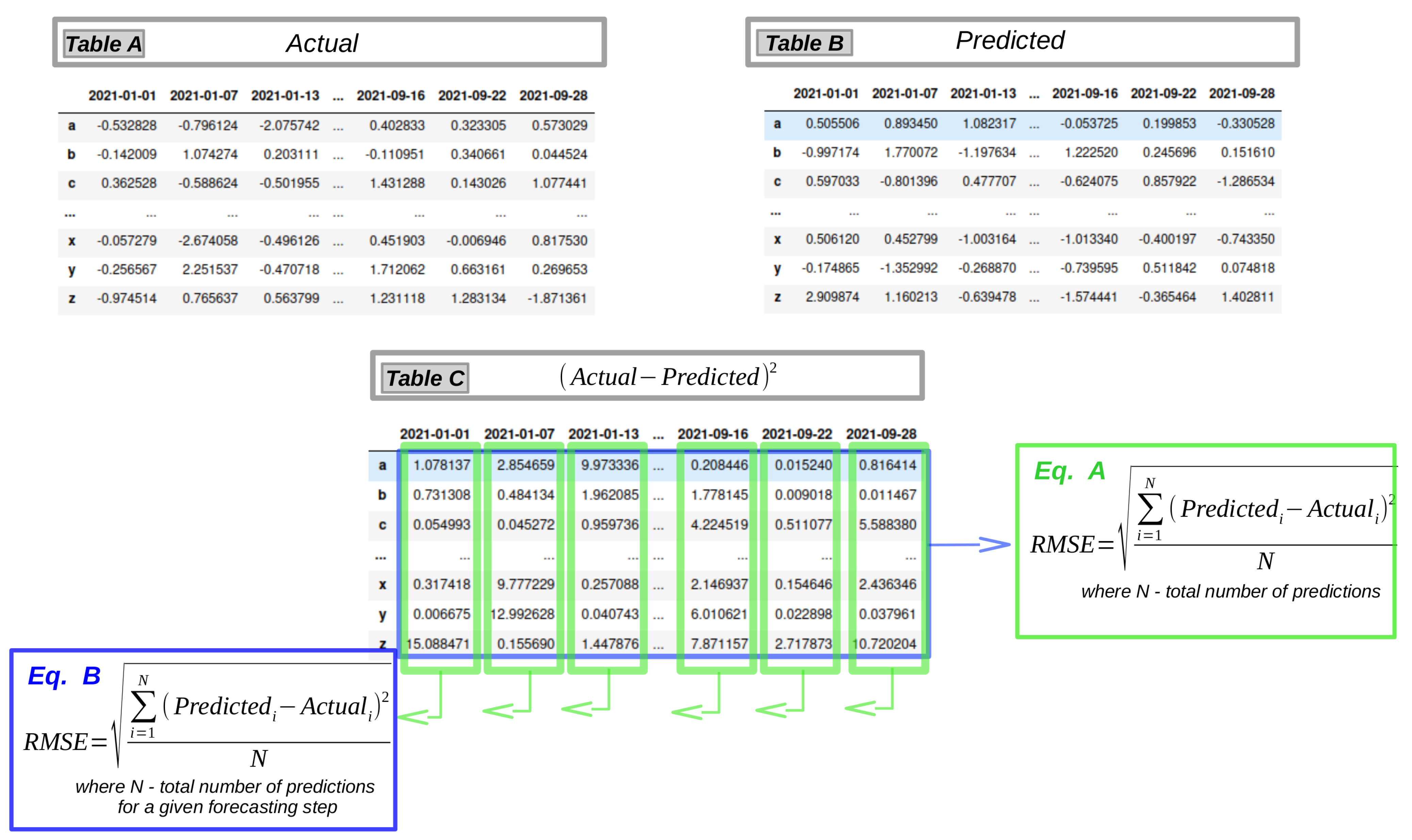
The models were evaluated with the use of Root Mean Square Error (RMSE) so the models with poor predictions (even rare) were penalized more. It is important to calculate this metric as a single value based on all predictions (Figure 4), and not as a mean or, more specifically, not as a median from the RMSE calculated separately for each profile or point. The importance of this approach is demonstrated on the basis of synthetic data in the Discussion section.
The following two RMSE calculation approaches were used for the analysis of the results as a general performance and as a function of the forecasting horizon: (1) Calculation as a single value based on all prediction data–this provided a general overview of how a given model performs on all control points (in space) and on all forecasting horizons (in time). (2) Calculation as a separate single value for each forecasting horizon—this allowed the performance of each model to be analyzed as a function of time.

4. Results

The underground mining activity undertaken in the LGCB area since the 1960s has significantly disturbed the equilibrium in the rock mass. As a consequence, a series of disadvantageous phenomena occur in the vicinity of the mining area [35]. These phenomena include continuous and discontinuous surface deformations. Apart from surface deformations caused by mineral extraction, mining tremors are also recorded [20,25,36].
The satellite radar data from the Sentinel 1 constellation led to the identification of 22 subsidence troughs, for which forecasts were subsequently performed on more than 10,000 points spatially located in 43 profiles. The forecasts of time series were performed on the basis of data on ground surface displacements at 6-day intervals, in the form of a single-step forecast (180 days ahead).
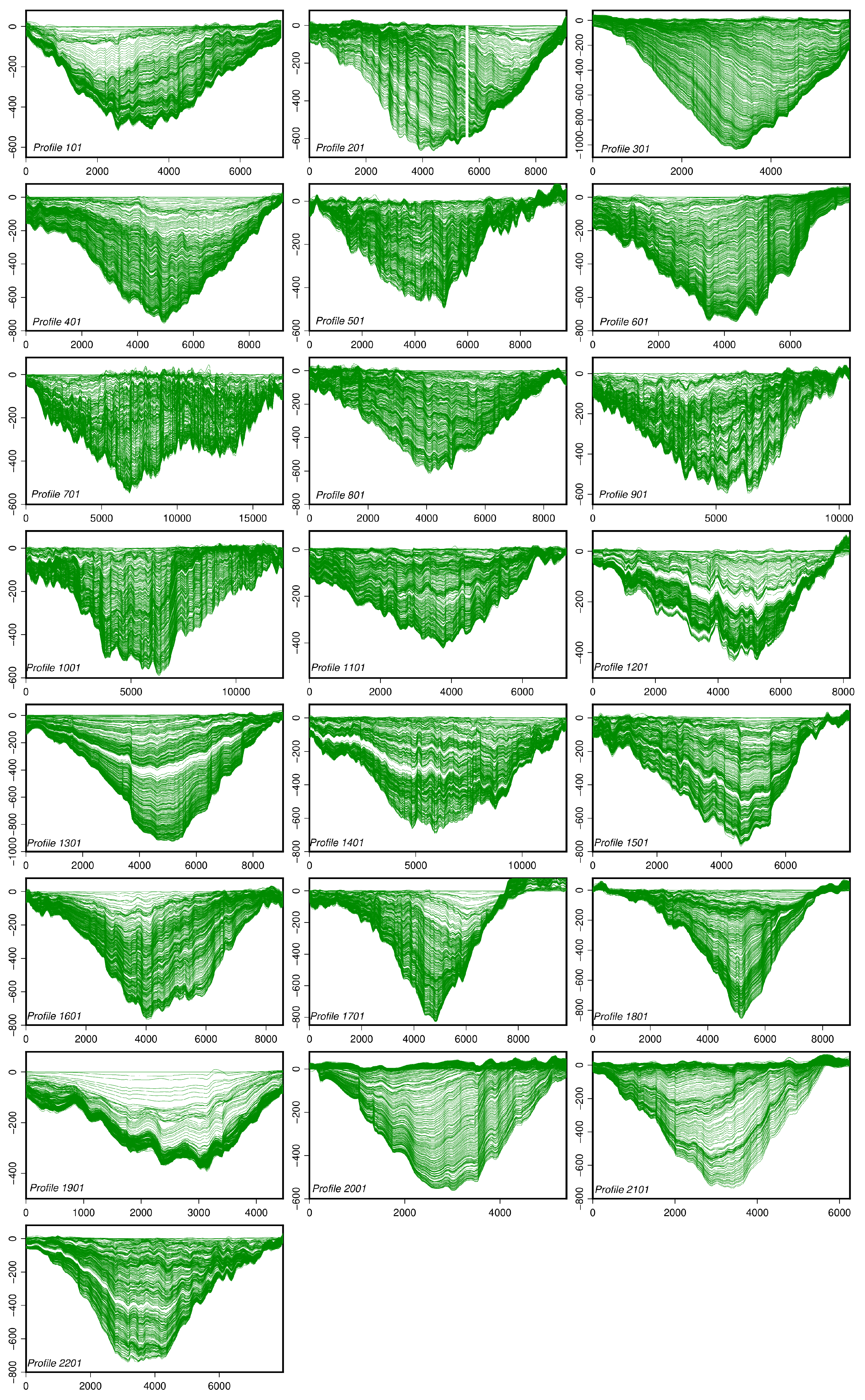
The results obtained as a result of calculating SAR data in a time series demonstrate quasi time-constant ground subsidence in the regions where copper ore is mined. The scale of this subsidence is a direct effect of the geographical range and intensity of a particular mining activity. The cumulative maximum displacement values recorded in trough 3, located in the north-western part of the Sieroszowice mining protective area reach −1060 mm (Figure 5). The mean 12-day subsidence increments are from −4 to −11 mm. The following observed deviating values are due to induced seismic events (please see profiles: 1201; 1301; 1401; 1501 and 2201, Figure 5). This fact has been confirmed in prior research [20].
In theory, the aim of mining forecasts is to determine the values of ground surface deformation indicators (subsidence, horizontal displacement, inclination, deformation) caused by the planned or already performed mining operations. In this particular case, the aim was to determine the forecast displacement values within the limits of all active subsidence troughs in the LGCB area and to evaluate the accuracy of the obtained results. The thus formulated task was the basis to provide a full description and evaluation of the forecast displacements. The analysis included both the points located in the centers of the troughs (i.e., showing maximum subsidence) and the points located on the borders of the troughs (showing minimum subsidence).
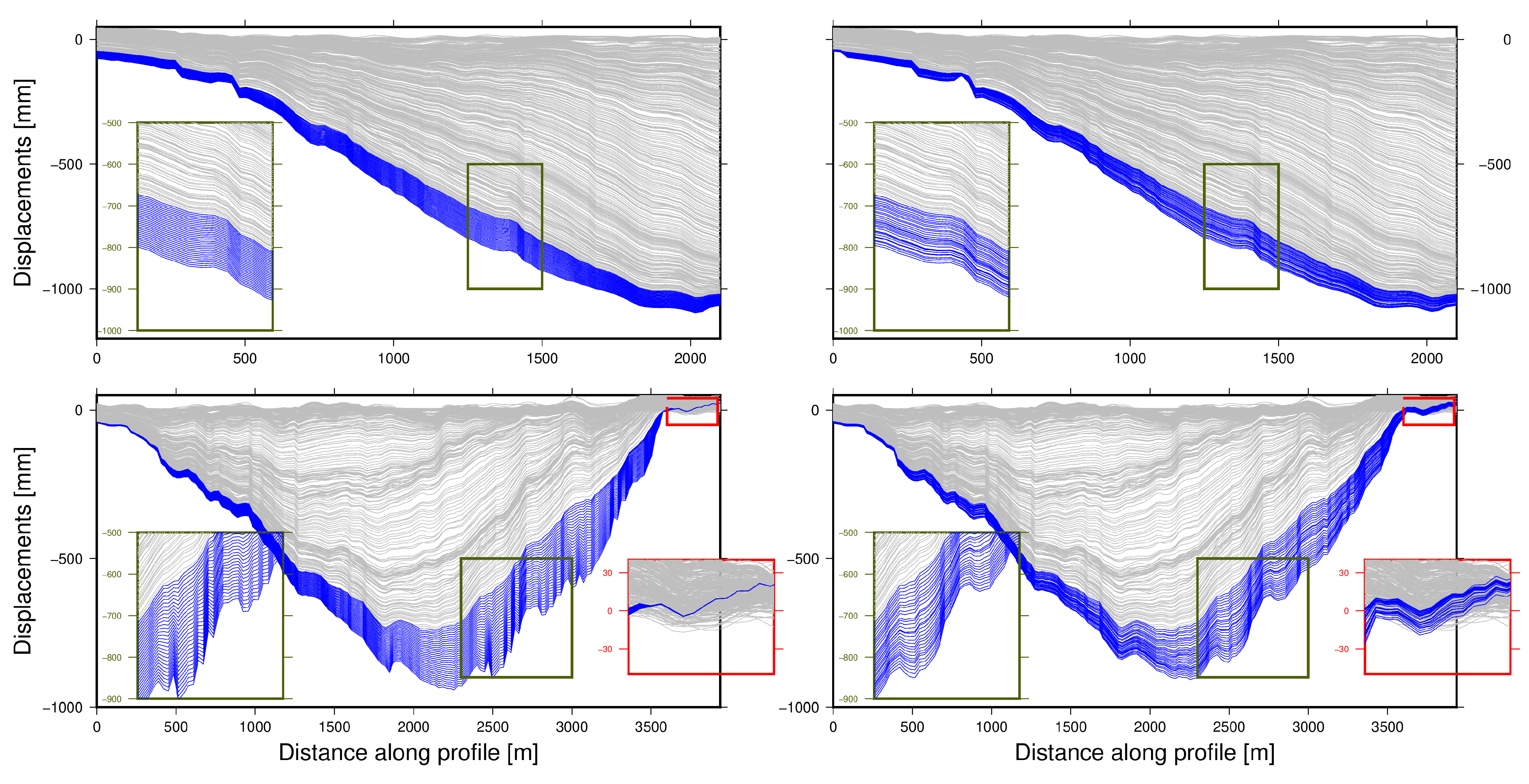
The obtained values of a single-step 180-day forecast demonstrate that the growth of the displacement field continues in all analyzed troughs (Figure 6). This fact is particularly visible in areas with the greatest mining impact (troughs No. 3, see Figure 5). It was observed that the forecast for subsequent 6-day displacement increments were coherent and did not intersect geometrically. Interestingly, the forecast results clearly “propagate information” about local disturbances in the subsidence processes (Figure 6, areas indicated with the green line). On the other hand, the limited forecast values for the trough borders have a significant error (Figure 6, areas indicated with the red line). This error is due to the fact that the SBAS displacement calculation method has the greatest error in these areas. The displacement forecast values are locally positive, which is in contrast to the actual situation.
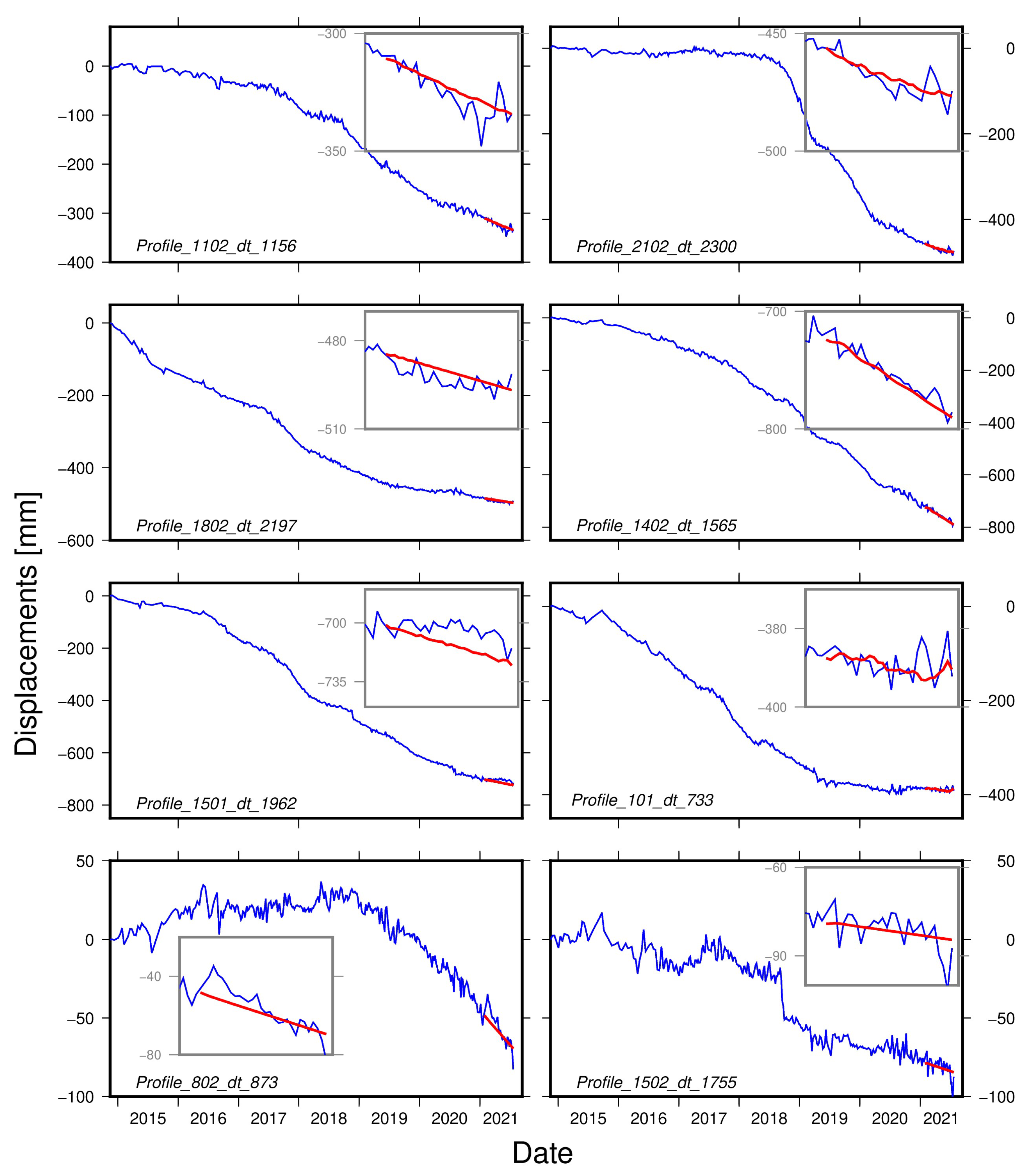
Figure 7 shows the forecasted displacement values calculated with the ARIMA model for randomly selected profiles. The slope of the forecasted values is similar to the actual values. However, the ARIMA model, which provided the most accurate results, did not detect local peaks and therefore its forecast deviates from the actual values.
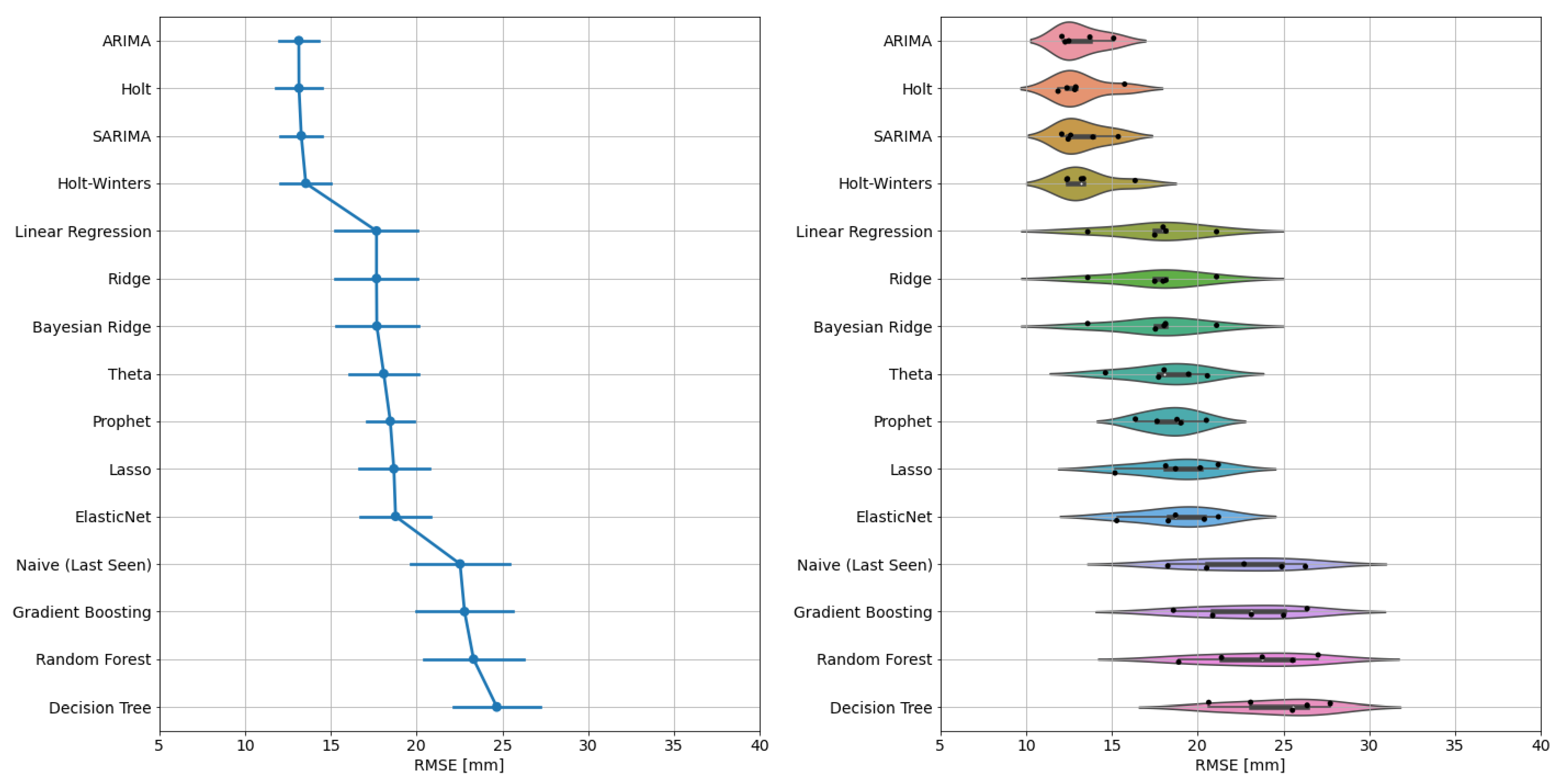
The metric of performance was Root Mean Square Error (RMSE) calculated on the basis of all samples from a given cross validation test window. Table 4 and Figure 8 show the results for each model and each CV test group (five groups). The performance metric obtained from the Naive forecasting strategy served as a baseline/reference. It allowed the relative improvement of the forecasts to be calculated as an absolute difference of RMSE and relative percentage improvement in comparison to the Naive approach.
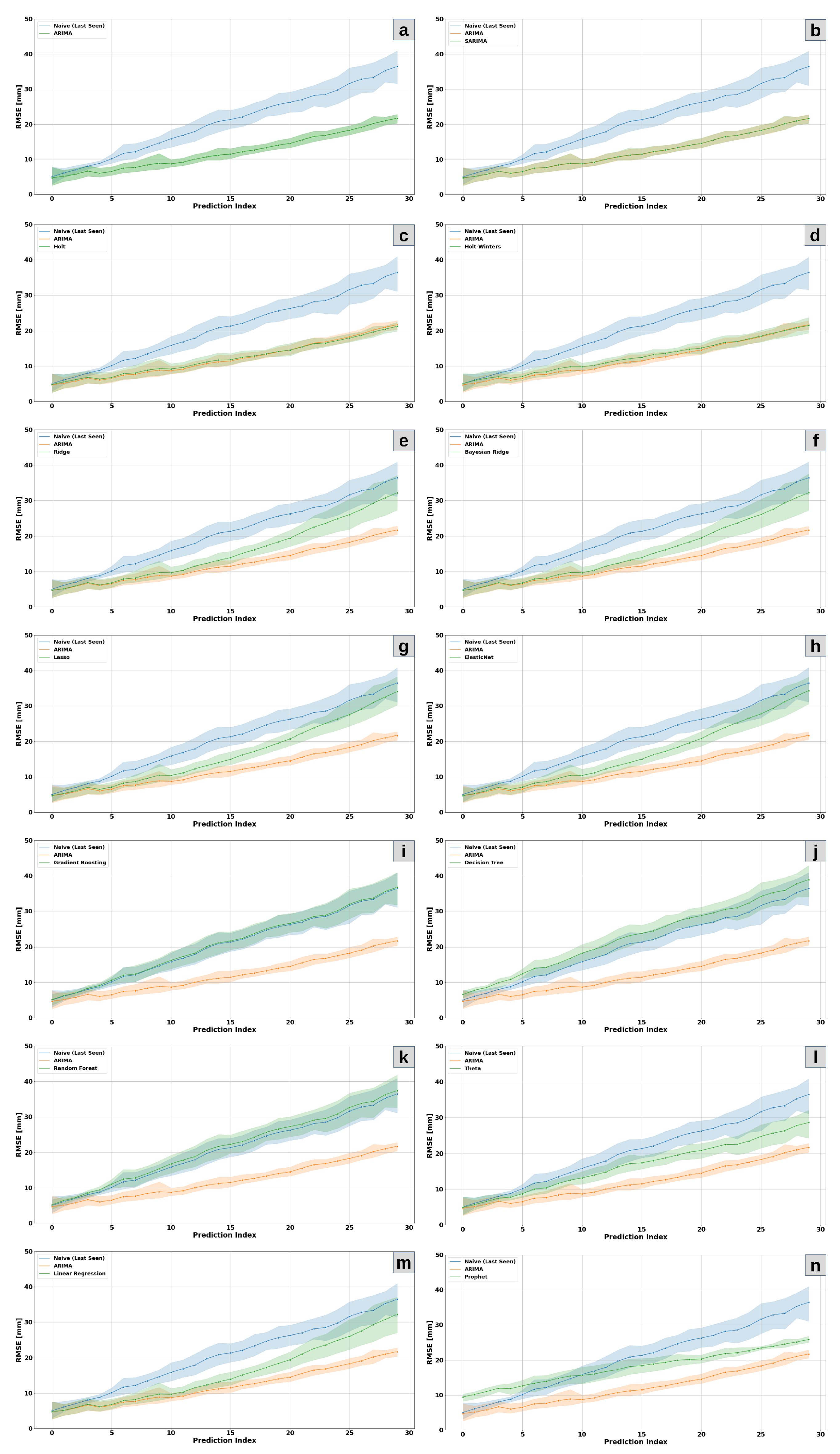
This is apparent in the visualization of the results (Figure 8). The group of methods including ARIMA, SARIMA, Holt and Holt-Winters showed the best performance. The results for this group are approx. 40% better than for the Naive approach. In order to better understand the model performance as a function of the forecasting horizon, the RMSE was calculated for each forecasting time step and CV group within this time step. Figure 9 shows the results as a function of the prediction time. On the X axis, there is a forecasting step as a number of days to the “future” (180 days). On the Y axis, there is the RMSE as a mean of all CV groups and its standard deviation as a shaded area around the mean. As can be observed, the prediction results for the ARIMA and Holt models are very similar over time and are not only significantly better than for the Naive approach but also much more stable (standard deviation does not change much over time). For the Naive approach, the RMSE increases much faster over time and its standard deviation increases as well.
Another group of models which provide significantly better results than the Naive approach are Linear Regression models (including regularized visions: Ridge, Bayesian Ridge, Lasso and ElasticNet). The results of Linear Regression as a function of forecasting time windows and a comparison to the Naive approach (baseline) and to the ARIMA (best mode) are presented in Figure 9a. It can be noted that short term forecasting results (up to 10 steps/60 days) are similar to the ARIMA results. Subsequently, the slope of the RMSE error changes and errors increase much faster for the longer forecasting horizons. The results for longer time periods are also less stable because standard deviation increases over time.
The group of Decision Tree-based models provided the worst results and its performance over time was not better than in the Naive approach. Figure 9i,j shows the results as a function of forecasting time for the Gradient Boosted and the Decision Trees models. The reason for this fact is that Decision Tree models are not able to extrapolate the predictions and instead they provide results only within the range of the target values observed on the training data. This means that DT-based models cannot be used as stand-alone models in these types of projects.
The present study focused on testing two more models (Prophet and Theta) which performed better than the Naive approach and provided a similar average RMSE calculated on the basis of all datapoints (see Figure 8). However, those models demonstrate a completely different behavior over time. Figure 9l shows the results for the Theta forecaster. The error trend line is consistent and follows a nearly central path between the Naive and ARIMA results. The results for Prophet are different (Figure 9n)—the short term results (up to 60 days) are actually worse than the results in the Naive approach, but the slope of the error curve is quite flat and the RMSE does not increase as quickly over time as for most of the tested models.

5. Discussion

This article presents a novel approach which consists of using results obtained with the SBAS method as data which can help in the identification of the influence of mining activity on the ground surface and subsequently when implementing this data as an input set for machine learning models. The current methods for forecasting the impact of mining activity on the ground surface on the one hand rely on a geometric representation of the problem [37,38,39], which allows the entire forecasting process to be based on a relatively small number of both dependent and independent variables. On the other hand, there is a group of numerical methods [40,41] which require precise models of the rock mass, physical and mechanical parameters of the geological and tectonic layers, and the parameters describing the mining process itself. The authors believe that machine learning algorithms can be classified between the above groups of forecasting methods.
The potential of synthetic aperture radar interferometry lies in this case mostly in the temporal resolution offered for obtaining new data. In the case of the Sentinel-1 mission, the current 12-day image-acquisition interval represents a regular source of data on the investigated phenomenon. Doubtlessly, this frequency is hardly achievable with traditional methods, except for on-ground systems which monitor changes in real time. InSAR methods also provide improved coverage of the investigated area with measurement points, which translates into larger ground surface displacement datasets to be used in machine learning algorithms.
Publications which have addressed this issue to date do not present results which are significantly more accurate than in the Naïve approach [7] (please see Figure 6). Nevertheless, our results are significantly more accurate for numerous models than the Naïve approach. This fact could be attributed to the character of the data obtained from the region and/or to the precise preparation of the data and to the implementation of a broad range of models. Many of these models proved more accurate than the Naïve approach; however, some of them provided less accurate results.
A comparison of the results from different machine learning algorithms suggests that the long-term linear trends are the greatest and most important factor, and this observation is consistent with prior works on the LGCB [20,26]. Interestingly, in the case of pairs of similar algorithms in which the first is only capable of forecasting trends (ARIMA, Holt), and the second is capable of predicting both trends and seasonal changes (SARIMA, Holt-Winters), the first algorithm provided better results (ARIMA better than SARIMA, and Holt better than Holt-Winters). This observation may suggest that seasonal changes are more random and that seasonal models are more susceptible to overfitting. The decision-tree (DT) models provided less accurate results and are not recommended as independent tools for analyzing this type of issues, in which extrapolation plays a significant role. However, the DT models may be used as components in hybrid models (comprising a number of algorithms), which will be the object of further research.
The authors believe that the choice of the method of selecting results and the selection of the metrics are of significance when estimating the accuracy of a forecast. In most cases, evaluations of the forecasts based on synthetic aperture radar interferometry involve estimations of the RMSE values. The range of the dataset required in RMSE calculations is selected differently [7,42]. In some cases, the metrics are not calculated from all observations, but rather as the mean or median of metrics calculated separately for each observation.
The RMSE calculation method proposed in this article is believed to provide an improved evaluation of the accuracies of displacement forecasts. As points with high errors have a greater influence on the RMSE value, it was calculated on the basis of all points as a whole. In a case where the majority of measurement points do not show significant displacements (e.g., they are located on the borders of the troughs), the value of the RMSE metrics calculated as a mean or a median [7] from all points will be unreliable and may be biased towards models which predict small or no displacement.
In this study, the RMSE is calculated on the basis of all data points. The difference is clearly visible in the following simple synthetic example (Table 5). A total of 11 random samples were generated with true and predicted values and a single RMSE value was calculated on the basis of all those samples. Subsequently, RMSE was calculated for each pair of points and the mean and the median were extracted from all of those values. Even in the case of normally distributed random samples, RMSE calculated on the basis of all points can be seen to be higher. In order to emphasize the difference, two outliers were introduced by simply adding 100 to the first two predicted values and the metrics were recalculated—the estimated error based on all samples is much higher in comparison to the error estimated with other methods.

6. Conclusions

Forecasting the impact of underground mining activity is one of the key issues in mineral mining. It is particularly important in cases where mining activity is performed in urban areas, where the negative influence of disturbing the rock mass may become a significant threat to both the overground and the underground infrastructure. This attempt at implementing machine learning algorithms in the forecasting of mining-related ground surface deformations offers a new perspective to the problem. The forecasting methods used to date rely on a geometric representation of the problem, which means the entire forecasting process is based on a relatively small number of both dependent and independent variables. On the other hand, numerical methods require precise models of the rock mass, physical and mechanical parameters of the geological and tectonic layers, and the parameters describing the mining process itself. The authors believe that the models based on machine learning may be classified between the two forecasting methods.
This article focuses on investigating the possibility of using satellite radar data in the long-term forecasting of displacements in mining protective areas. The best results were obtained with the use of the ARIMA and Holt models. The accuracy was evaluated with the use of RMSE, which was calculated on the basis of all samples from a particular cross-validation test window. This approach led to the forecasts’ improvement in terms of the absolute RMSE difference and as a percentage in comparison with the Naive approach.
The analysis of deformations in the LGCB mining protective areas involved a relatively large area of almost 500 km 2 . Some of the identified subsidence troughs are located in urban areas or in the vicinity of key infrastructure objects. The presented results of ground surface displacement forecasts based on SAR data and on machine learning have been demonstrated to represent an alternative to the currently employed methods of forecasting mining-induced ground surface deformations.
Many of the tested models provided results that are more accurate than those of the Naïve approach, which is advantageous when compared with the publications to date. The authors consider this fact to be promising and see potential for further improvement. As the models in this research were used to analyze only the data from the SBAS method, the authors believe that the next natural step in further research will be to use new types of data, with geological, geotectonic, mining and man-made activities as additional features in constructing the models. Such an approach will facilitate not only a comparison of the accuracy of models using InSAR results and models using InSAR results together with mining, geological and hydrogeological information, but also a verification of which features have the greatest influence on the accuracy of the predictions.

Author Contributions

Conceptualization, K.C. and W.M.; Formal analysis, K.C. and W.M.; Investigation, K.C. and W.M.; Methodology, K.C. and W.M.; Project administration, K.C. and W.M.; Resources, K.C. and W.M.; Validation, K.C. and W.M.; Visualization, K.C. and W.M.; Writing—original draft, K.C. and W.M.; Writing—review & editing, K.C. and W.M.; All authors have read and agreed to the published version of the manuscript.

Funding

Calculations have been carried out using resources provided by Wroclaw Centre for Networking and Supercomputing (http://wcss.pl (accessed on 14 February 2022)),grant No. 345 and servers from trainAI GmbH.

Data Availability Statement

Not applicable.

Conflicts of Interest

The authors declare no conflict of interest.

References

  1. Schumann, G.J.P.; Frye, S.; Wells, G.; Adler, R.; Brakenridge, R.; Bolten, J.; Murray, J.; Slayback, D.; Policelli, F.; Kirschbaum, D.; et al. Unlocking the full potential of Earth observation during the 2015 Texas flood disaster. Water Resour. Res. 2016, 52, 3288–3293. [Google Scholar] [CrossRef]
  2. Schumann, G.J.P.; Brakenridge, G.R.; Kettner, A.J.; Kashif, R.; Niebuhr, E. Assisting Flood Disaster Response with Earth Observation Data and Products: A Critical Assessment. Remote Sens. 2018, 10, 1230. [Google Scholar] [CrossRef]
  3. Cozannet, G.L.; Kervyn, M.; Russo, S.; Speranza, C.I.; Ferrier, P.; Foumelis, M.; Lopez, T.; Modaressi, H. Space-Based Earth Observations for Disaster Risk Management. Surv. Geophys. 2020, 41, 1209–1235. [Google Scholar] [CrossRef]
  4. Nemni, E.; Bullock, J.; Belabbes, S.; Bromley, L. Fully Convolutional Neural Network for Rapid Flood Segmentation in Synthetic Aperture Radar Imagery. Remote Sens. 2020, 12, 2532. [Google Scholar] [CrossRef]
  5. Naghibi, S.A.; Khodaei, B.; Hashemi, H. An integrated InSAR-machine learning approach for ground deformation rate modeling in arid areas. J. Hydrol. 2022, 608, 127627. [Google Scholar] [CrossRef]
  6. Anantrasirichai, N.; Biggs, J.; Albino, F.; Bull, D. A deep learning approach to detecting volcano deformation from satellite imagery using synthetic datasets. Remote Sens. Environ. 2019, 230, 111179. [Google Scholar] [CrossRef]
  7. Hill, P.; Biggs, J.; Ponce-López, V.; Bull, D. Time-Series Prediction Approaches to Forecasting Deformation in Sentinel-1 InSAR Data. J. Geophys. Res. Solid Earth 2021, 126, e2020JB020176. [Google Scholar] [CrossRef]
  8. Carlà, T.; Intrieri, E.; Raspini, F.; Bardi, F.; Farina, P.; Ferretti, A.; Colombo, D.; Novali, F.; Casagli, N. Perspectives on the prediction of catastrophic slope failures from satellite InSAR. Sci. Rep. 2019, 9, 14137. [Google Scholar] [CrossRef]
  9. Strzałkowski, P.; Szafulera, K. Occurrence of Linear Discontinuous Deformations in Upper Silesia (Poland) in Conditions of Intensive Mining Extraction—Case Study. Energies 2020, 13, 1897. [Google Scholar] [CrossRef]
  10. Cała, M.; Tajduś, A.; Andrusikiewicz, W.; Kowalski, M.; Kolano, M.; Stopkowicz, A.; Cyran, K.; Jakóbczyk, J. Long term analysis of deformations in salt mines: Kłodawa salt mine case study, central Poland. Arch. Min. Sci. 2017, 62, 565–577. [Google Scholar] [CrossRef] [Green Version]
  11. Milczarek, W. Application of PSInSAR for assessment of surface deformations in post_mining area _ case study of the former Walbrzych Hard Coal Basin (SW Poland). Acta Geodyn. Geomater. 2017, 14, 185. [Google Scholar] [CrossRef]
  12. Henderson, S.T.; Pritchard, M.E. Decadal volcanic deformation in the Central Andes Volcanic Zone revealed by InSAR time series. Geochem. Geophys. Geosyst. 2013, 14, 1358–1374. [Google Scholar] [CrossRef]
  13. Albino, F.; Biggs, J.; Yu, C.; Li, Z. Automated Methods for Detecting Volcanic Deformation Using Sentinel-1 InSAR Time Series Illustrated by the 2017–2018 Unrest at Agung, Indonesia. J. Geophys. Res. Solid Earth 2020, 125, e2019JB017908. [Google Scholar] [CrossRef]
  14. Xu, X.; Sandwell, D.T.; Tymofyeyeva, E.; Gonzalez-Ortega, A.; Tong, X. Tectonic and anthropogenic deformation at the Cerro Prieto geothermal step-over revealed by sentinel-1A InSAR. IEEE Trans. Geosci. Remote Sens. 2017, 55, 5284–5292. [Google Scholar] [CrossRef]
  15. Yang, Z.; Li, Z.; Zhu, J.; Wang, Y.; Wu, L. Use of SAR/InSAR in Mining Deformation Monitoring, Parameter Inversion, and Forward Predictions: A Review. IEEE Geosci. Remote Sens. Mag. 2020, 8, 71–90. [Google Scholar] [CrossRef]
  16. Yang, Q.; Zhao, W.; Dixon, T.H.; Amelung, F.; Han, W.S.; Li, P. InSAR monitoring of ground deformation due to CO2 injection at an enhanced oil recovery site, West Texas. Int. J. Greenh. Gas Control 2015, 41, 20–28. [Google Scholar] [CrossRef]
  17. Ojha, C.; Werth, S.; Shirzaei, M. Recovery of aquifer-systems in Southwest US following 2012–2015 drought: Evidence from InSAR, GRACE and groundwater level data. J. Hydrol. 2020, 587, 124943. [Google Scholar] [CrossRef]
  18. Carreño Conde, F.; De Mata Muñoz, M. Flood Monitoring Based on the Study of Sentinel-1 SAR Images: The Ebro River Case Study. Water 2019, 11, 2454. [Google Scholar] [CrossRef]
  19. Friedl, P.; Seehaus, T.; Braun, M. Sentinel-1 Ice Surface Velocities of Svalbard. 2021. Available online: https://datapub.gfz-potsdam.de/download/10.5880.FIDGEO.2021.016nuviews/ (accessed on 26 May 2022). [CrossRef]
  20. Milczarek, W. Application of a Small Baseline Subset Time Series Method with Atmospheric Correction in Monitoring Results of Mining Activity on Ground Surface and in Detecting Induced Seismic Events. Remote Sens. 2019, 11, 1108. [Google Scholar] [CrossRef] [Green Version]
  21. Samsonov, S.; d’Oreye, N.; Smets, B. Ground deformation associated with post-mining activity at the French–German border revealed by novel InSAR time series method. Int. J. Appl. Earth Obs. Geoinf. 2013, 23, 142–154. [Google Scholar] [CrossRef]
  22. Blachowski, J.; Kopeć, A.; Milczarek, W.; Owczarz, K. Evolution of Secondary Deformations Captured by Satellite Radar Interferometry: Case Study of an Abandoned Coal Basin in SW Poland. Sustainability 2019, 11, 884. [Google Scholar] [CrossRef]
  23. Rouet-Leduc, B.; Hulbert, C.; Lubbers, N.; Barros, K.; Humphreys, C.J.; Johnson, P.A. Machine Learning Predicts Laboratory Earthquakes. Geophys. Res. Lett. 2017, 44, 9276–9282. [Google Scholar] [CrossRef]
  24. Gaddes, M.E.; Hooper, A.; Bagnardi, M. Using Machine Learning to Automatically Detect Volcanic Unrest in a Time Series of Interferograms. J. Geophys. Res. Solid Earth 2019, 124, 12304–12322. [Google Scholar] [CrossRef]
  25. Milczarek, W.; Kopeć, A.; Głąbicki, D.; Bugajska, N. Induced Seismic Events—Distribution of Ground Surface Displacements Based on InSAR Methods and Mogi and Yang Models. Remote Sens. 2021, 13, 1451. [Google Scholar] [CrossRef]
  26. Ilieva, M.; Rudziński, Ł.; Pawłuszek-Filipiak, K.; Lizurek, G.; Kudłacik, I.; Tondaś, D.; Olszewska, D. Combined Study of a Significant Mine Collapse Based on Seismological and Geodetic Data—29 January 2019, Rudna Mine, Poland. Remote Sens. 2020, 12, 1570. [Google Scholar] [CrossRef]
  27. Berardino, P.; Fornaro, G.; Lanari, R.; Sansosti, E. A new algorithm for surface deformation monitoring based on small baseline differential {SAR} interferograms. IEEE Trans. Geosci. Remote Sens. 2002, 40, 2375–2383. [Google Scholar] [CrossRef]
  28. Tymofyeyeva, E.; Fialko, Y. Mitigation of atmospheric phase delays in InSAR data, with application to the eastern California shear zone. J. Geophys. Res. Solid Earth 2015, 120, 5952–5963. [Google Scholar] [CrossRef]
  29. Carlà, T.; Intrieri, E.; Traglia, F.D.; Casagli, N. A statistical-based approach for determining the intensity of unrest phases at Stromboli volcano (Southern Italy) using one-step-ahead forecasts of displacement time series. Nat. Hazards 2016, 84, 669–683. [Google Scholar] [CrossRef]
  30. Sompolski, M.; Tympalski, M.; Kopeć, A.; Milczarek, W. Application of the autoregressive integrated moving average (ARIMA) model in prediction of mining ground surface displacement. In Proceedings of the EGU General Assembly 2022, Vienna, Austria, 23–27 May 2022. EGU22-12697. [Google Scholar] [CrossRef]
  31. Moretto, S.; Bozzano, F.; Mazzanti, P. The Role of Satellite InSAR for Landslide Forecasting: Limitations and Openings. Remote Sens. 2021, 13, 3735. [Google Scholar] [CrossRef]
  32. Desjardins, M.; de Graaf, P. InSAR monitoring guidelines: Using simple to use decision trees—An owner’s perspective. In Proceedings of the SSIM 2021: Second International Slope Stability in Mining, Perth, Australia, 26–28 October 2021; Dight, P., Ed.; Australian Centre for Geomechanics: Crawley, Australia, 2021; pp. 185–198. [Google Scholar] [CrossRef]
  33. Zhao, F.; Meng, X.; Zhang, Y.; Chen, G.; Su, X.; Yue, D. Landslide Susceptibility Mapping of Karakorum Highway Combined with the Application of SBAS-InSAR Technology. Sensors 2019, 19, 2685. [Google Scholar] [CrossRef]
  34. Wang, L.; Yang, J.; Shi, L.; Li, P.; Zhao, L.; Deng, S. Impact of Backscatter in Pol-InSAR Forest Height Retrieval Based on the Multimodel Random Forest Algorithm. IEEE Geosci. Remote Sens. Lett. 2020, 17, 267–271. [Google Scholar] [CrossRef]
  35. Antonielli, B.; Sciortino, A.; Scancella, S.; Bozzano, F.; Mazzanti, P. Tracking Deformation Processes at the Legnica Glogow Copper District (Poland) by Satellite InSAR—I: Room and Pillar Mine District. Land 2021, 10, 653. [Google Scholar] [CrossRef]
  36. Kudłacik, I.; Kapłon, J.; Lizurek, G.; Crespi, M.; Kurpiński, G. High-rate GPS positioning for tracing anthropogenic seismic activity: The 29 January 2019 mining tremor in Legnica- Głogów Copper District, Poland. Measurement 2021, 168, 108396. [Google Scholar] [CrossRef]
  37. Knothe, S. Effect of time on formation of basin subsidence. Arch. Min. Steel Ind. 1953, 1, 1–7. [Google Scholar]
  38. Kowalski, A. Surface subsidence and rate of its increaments based on measurements and theory. Arch. Min. Sci. 2001, 46, 391–406. [Google Scholar]
  39. Zhang, L.; Cheng, H.; Yao, Z.; Wang, X. Application of the Improved Knothe Time Function Model in the Prediction of Ground Mining Subsidence: A Case Study from Heze City, Shandong Province, China. Appl. Sci. 2020, 10, 3147. [Google Scholar] [CrossRef]
  40. Sikora, P.; Wesołowski, M. Numerical assessment of the influence of former mining activities and plasticity of rock mass on deformations of terrain surface. Int. J. Min. Sci. Technol. 2021, 31, 209–214. [Google Scholar] [CrossRef]
  41. Dudek, M.; Tajduś, K. FEM for prediction of surface deformations induced by flooding of steeply inclined mining seams. Geomech. Energy Environ. 2021, 28, 100254. [Google Scholar] [CrossRef]
  42. Radman, A.; Akhoondzadeh, M.; Hosseiny, B. Integrating InSAR and deep-learning for modeling and predicting subsidence over the adjacent area of Lake Urmia, Iran. Gisci. Remote Sens. 2021, 58, 1413–1433. [Google Scholar] [CrossRef]
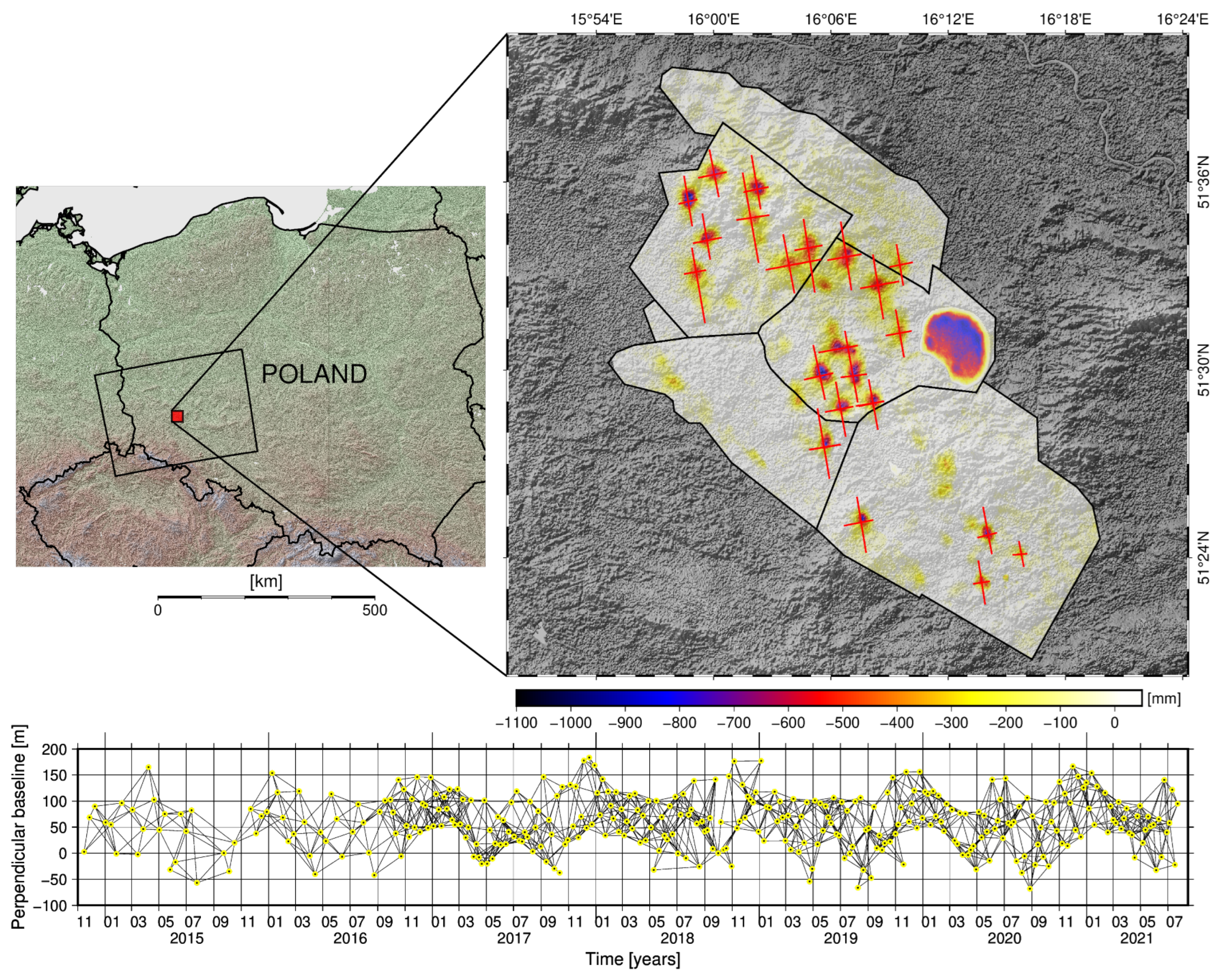
Figure 1. Location of the research area and the displacement results calculated with the SBAS method Red lines represent profiles located within the borders of the largest identified subsidence troughs. Each of the profiles is represented by a set of points used in forecasts. The lower part comprises a graph of baselines for the SBAS calculations of the radar data.
Remotesensing 14 04755 g001
Figure 2. Locations of profiles for the identified subsidence troughs (indicated in green). The results are presented in the satellite system (range/azimuth). The range profiles are indicated in blue, and the azimuth profiles are indicated in red.
Remotesensing 14 04755 g002
Figure 3. Graphical representation of cross validation used for the analyzed SAR data calculations with the use of the SBAS method.
Remotesensing 14 04755 g003
Figure 4. Schematic RMSE calculation method on the basis of synthetic data, following two approaches: as a result from all observations (pattern A—on the right), as a result from the observations which belong to only one time window (pattern B—on the left). Table A contains information about the current state of data in the points (top left corner); Table B contains information with the result of machine learning predictions (top right corner); Table C provides the quadratic difference of the current state and the prediction for each point in time (below).
Remotesensing 14 04755 g004
Figure 5. Results of ground surface displacement calculations performed with the SBAS method from November 2014 to July 2021. The presented results apply to horizontal profiles indicated in Figure 2.
Remotesensing 14 04755 g005
Figure 6. Representative forecast results for the 3rd (bottom) and 21st (top) subsidence troughs: for the ARIMA model (on the left) and for the Holt model (on the right). Featured and enlarged areas (green polygons) show increments dynamics of the forecast results. The areas bounded by the red polygon show displacement forecasts are locally positive, which is in contrast to the actual situation.
Remotesensing 14 04755 g006
Figure 7. ARIMA forecast results for randomly selected profiles.
Remotesensing 14 04755 g007
Figure 8. RMSE calculation results on the basis of the data from all points and time windows (pattern a from Figure 4). The visualization on the left shows the results as a pointplot with the mean and standard deviation values from all five cross validation groups per model. The visualization on the right shows the results as a violinplot from all five cross validation groups per model. Based on the above visualizations, the models can be classified into three groups by their performance in comparison with the Naive approach. Group with the best results includes the following models: ARIMA, Holt, SARIMA and Holt-Winters. Another group which provides results better than the Naive approach, but a worse ARIMA and Holt than group includes the following models: Linear Regression, Ridge, Theta, Prophet, Lasso and ElasticNet. The last group does not provide better results than the Naive approach and includes models based on decision trees (Gradient Boosting, Random Forest and Decision Tree).
Remotesensing 14 04755 g008
Figure 9. RMSE calculation results on the basis of the data from all points for a particular prediction window (Equation (B) from Figure 4). The accuracy of the model is visually represented as a function of time (forecasting horizon). For reference, each of the plots includes the results of the Naive approach (baseline) and of the ARIMA model which provided the best results. The plots present the mean from all cross-validation groups (solid line) for a particular prediction window, along with its 95% confidence interval in the form of a ribbon around the mean. The following plots present the results for (a) ARIMA model, (b) SARIMA model, (c) Holt model, (d) Holt-Winters model, (e) Ridge model, (f) Bayesian Ridge model, (g) Lasso model, (h) ElasticNet model, (i) Gradient Boosting, (j) Decision Tree, (k) Random Forest, (l) Theta model, (m) Linear Regression model and (n) Prophet model, respectively.
Remotesensing 14 04755 g009
Table 1. Basic information of SAR data and SBAS results used in forecasting.
Calculation period15 November 2014–23 July 2021
AensorsSentinel 1A/B
orbit no./IW no.73/IW2
Number of images295
Average interval between acquisitions12 days (until October 2016); 6 days (until July 2021)
Perpendicular baseline/time baseline50 m/50 days
Number of interferograms1343
Table 2. Basic information of SAR data and SBAS results used in forecasting. The third column includes literature references (if applicable).
MethodDefinitionRef.
NaiveThe use of the prior/last period in forecasting the next period is the easiest forecasting method.
ARIMAA common forecasting method for single-variant time series; it can be used if the time series is stationary.[29,30]
SARIMAUsed in analyzing time series with a trend and seasonal variability—it allows for seasonal patterns.[7]
LinearA linear regression model; it is based on an assumed linear relationship.
Regressionbetween the forecasted variable and a single prediction variable.[8,31]
RidgeA linear regression model; expansion of linear regression by modifying
Regressionthe loss function. (reduction in the model’s complexity)
Bayesian RidgeA linear regression model with the L2 regularization.
LassoA type of linear regression employing shrinking which consists of
Regressionthe reduction in the data values towards the central point (e.g., the mean); it employs the L1.
ElasticNetA linear regression model; combines the properties of the Ridge
Regressionand Lasso models.
ThetaA forecasting method which consists of matching two lines and forecasting the lines with the use of simple exponential smoothing followed by combining the forecasts from the two lines in order to obtain the final forecast.
Holt-WintersA group of exponential smoothing models; it is capable of “handling” time series characterized by both a trend and seasonal variability.
HoltA group of exponential smoothing models
Decision TreeUsed in predictive modeling of classification and regression[5,32]
GradientBoosted decision trees used in predictive modeling of classification
Boostingand regression.[5]
Random ForestBagged decision trees, used in predictive modeling of classification and regression; forecasts time series (supervised training); requires step validation.[33,34]
ProphetForecasts data in time series based on an additive model, in which non-linear trends are matched to a defined period; Prophet was released by the Core Data Science team from Facebook.
Table 3. Temporal summary of cross validation test windows.
CV No.CV-1CV-2CV-3CV-4CV-5
Time range of the following10 February 20199 August 20195 February 20203 August 202030 January 2021
test groups (start-end)3 August 201930 January 202028 July 202024 January 202123 July 2021
Table 4. Comparison of the calculated errors for all analyzed models.
ModelCV-1CV-2CV-3CV-4CV-5MeanMedianNaive
Improvement
[mm]
Naive
Improvement
[%]
ARIMA12.0812.2713.7115.1012.4813.1312.48−9.40−41.73
Holt12.3812.8412.8915.7411.8613.1412.84−9.39−41.69
SARIMA12.0712.4513.8915.3712.5913.2812.59−9.26−41.09
Holt-Winters12.4113.3413.2216.3512.3813.5413.22−9.00−39.92
Linear Regression17.9813.5921.1018.1417.5017.6617.98−4.87−21.62
Ridge17.9813.5921.1018.1417.5017.6617.98−4.87−21.62
Bayesian Ridge18.0513.5921.1018.1317.5417.6818.05−4.86−21.55
Theta20.5719.4718.0417.7214.6218.0818.04−4.45−19.75
Prophet19.0216.3720.5117.6418.7918.4718.79−4.07−18.06
Lasso18.1415.1821.2020.1518.7118.6818.71−3.86−17.13
ElasticNet18.2915.2821.2120.3918.7118.7718.71−3.76−16.69
Naive (Last Seen)26.2824.9022.7120.5218.2622.5422.710.000.00
Gradient Boosting26.3825.0123.1320.8818.5922.8023.130.261.16
Random Forest27.0225.5423.7721.3918.8923.3223.770.793.49
Decision Tree27.7326.3825.5323.0920.6424.6725.532.149.50
Table 5. Comparison of RMSE results for the actual and the synthetic data.
No OutliersWith Outliers
y_truey_predRMSEy_truey_predRMSE
0.1554-0.09110.24640.155499.908999.7536
0.19920.68580.48660.1992100.685100.4866
−1.4259−2.58141.1555−1.4259−2.58141.1555
−0.28310.16510.4482−0.28310.16510.4482
−0.5662−0.26640.2998−0.5662−0.26640.2998
1.2243−0.61561.83991.2243−0.61561.8399
2.1519−2.67254.82442.1519−2.67254.8244
−0.8778−1.75280.875−0.8778−1.75280.875
−1.28630.0831.3694−1.28630.0831.3694
−0.49850.02640.525−0.49850.02640.525
0.45850.30880.14970.45850.30880.1497
RMSE based on all samples = 1.09RMSE based on all samples = 42.91
mean from RMSE of each point = 0.91mean from RMSE of each point = 18.99
median from RMSE of each point = 1.03median from RMSE of each point = 1.09
Publisher’s Note: MDPI stays neutral with regard to jurisdictional claims in published maps and institutional affiliations.