Abstract
The radio propagation loss prediction model is essential for maritime communication. The oceanic tropospheric duct is much more complicated than the atmospheric structure on land due to the rough sea surface influence, and it leads to difficulties in loss prediction. Classical radio wave propagation loss prediction models are either based on complicated electromagnetic wave theories or rely on empirical data. Consequently, they suffer from low accuracy and a limited range of application. To address this issue, a novel maritime propagation loss prediction approach is proposed, which fully exploits the data for training. In this new approach, 3D sea surface contour profiles are generated based on the Pierson–Moskowitz spectrum theory and the direction expansion formula Stereo Wave Observation Program (SWOP), by sweeping the parameters. The full-wave propagation procedure of radio signals over the sea surface is simulated by commercial EM analysis software CST Studio Suite. Based on the large quantity of simulated data, the BP neural network is employed to fit the radio propagation loss and obtain the sea surface radio wave propagation prediction model. Other classical machine learning methods are also compared to validate the proposed approach. Traditional empirical model construction relies on observation data. This approach, for the first time, proposed an automatic scheme which covers the whole procedure from the data generation to prediction model training. It avoids the requirements for on-site observation, as well as significantly decreases the cost of experiments. The application scope of the prediction model such as propagation distance range and working frequency range could be adaptive through adjustments for simulated sea size and simulated working frequency. This approach is validated to save 99% of prediction time in comparison with the full-wave simulations. The prediction model trained via our proposed method could obtain the coefficient of determination R2 which is over 0.92, demonstrating the superiority of this method.
1. Introduction
The propagation of radio waves in the atmospheric duct and in water at sea have always drawn great attention [1,2,3,4,5,6,7]. The former is related to ocean communication, while the latter has applications such as mineral exploration and submarine detection and communication. However, the propagation in the oceanic duct layer is rarely discussed, mainly due the complicated electromagnetic environment characteristics.
During the propagation process, the propagation environment leads to great prediction difficulties. It is mainly influenced by the weather, which causes evaporative waveguides, rainfall interference, and the irregular propagation path which is also known as rough sea. The rough sea combined with the upper bound of the atmosphere results in oceanic tropospheric duct phenomena, which are not included in loss prediction on land [8].
The most important application of radio propagation over the sea is the communication between maritime ships [9,10]. The communication frequency between ships is generally high, and the distance is relatively close compared to the physical scale of the ocean. As a consequence, the radio does not propagate through the atmospheric duct. At the same time, the height of the communication antenna on ships is generally between a few meters to a dozen meters, so radio waves will be absorbed and reflected by the sea surface. The reflection and scattering effect from the sea surface will result in multipath components between transmitting and receiving antennas. The random phase and amplitudes of different multipath components cause fluctuations in signal strength, thereby inducing small-scale fading [11]. To take the rough sea factor into consideration, the existed prediction models are yet to be revised.
Since the 1950s, research on radio wave propagation model is mainly based on land wireless communication and divided into analytical model, empirical model and analytical-empirical combined model. Early analytical formulations were mostly established based on the assumption of ray tracing [12] representations in two dimensions (2D) or over a smooth spherical earth through homogeneous (standard) atmosphere [13,14,15,16,17]. The complex boundary effects of electromagnetic wave refraction and reflection for a rough sea surface limits the application of analytical models. Empirical models such as the Okumura–Hata model [18,19] and Egli model [20] build formulas based on data obtained from long-term radio propagation observation on the main-land. As a result, the empirical model is not applicable when analyzing radio propagation over the sea. Analytical–empirical combined models utilize both analytical theory and observation data to build simple models such as the Longley–Rice [21] model and the ITU-R P 1546 [22] model, but they ignore traditional high-frequency (HF) communication and the irregular sea surface due to the wind. According to [23], the propagation loss is proportional to irregular parameters during line-of-sight propagation. It is necessary to take terrain into consideration when the sea wind speed is relatively high.
In order to make up for the deficiencies in the analytical or empirical models and the full wave calculation methods of radio propagation on the sea surface, this paper conducts the research of seeking an efficient and accurate surrogate model to predict the electromagnetic wave propagation loss over the sea. This model contains major important parameters which can affect the path loss, such as the wind speed vector, the locations of the ships, and the height of the antennas. This paper proposes for the first time to construct a three-dimensional sea surface model based on the theory of ocean wave spectrum, so as to simulate the full wave process of radio propagation on the sea surface to construct the data set with high fidelity, and then use machine learning methods to establish the surrogate radio wave propagation loss model on the sea surface.
Two-dimensional ocean surface establishment has a mature ground theory. General approaches to simulate sea surface can be divided into three different categories. The first is based on the physical characteristics of ocean waves utilizing the Navier–Stokes equation and calculating the moving state of each particle [24]. The second method starts from the geometric shape of the waves and uses geometric curves or surfaces to represent the surface of the waves according to the geometric shapes of the waves and sets the parameter values of various attributes of the waves artificially, so as to generate various types of wave data on the computer. The typical methods of this modeling technology include the bump mapping method, the modeling method based on the Stokes model, the modeling method based on the Pachey model, and the modeling method based on the Gerstner model [25]. The third method is the wave-spectrum-based approach. It regards the random waves as a random process, which means a random wave can be represented as the sum of many random components. This method was proposed in the 1940s by oceanographers Neuman and Pierson et al. At present, the mature stochastic wave models include the Pierson model [26], the Longuet–Higgins model [27], and the Fourier–Stieltjes integral model [28], etc. Jensen [29] and Tessendorf [30] described in detail the use of ocean statistics and empirical models, respectively, using a series of superpositions of sine waves to simulate the sea surface and quickly generating a height field simulation similar to the wave spectrum distribution through Fast Fourier transform (FFT). Jocelyn [31] uses the Gerstner model based on the wave spectrum and the Fourier transform method to simulate waves in deep water.
The rapid development of simulation software for electromagnetic waves offers possibilities of full-wave simulations in three-dimensional space. The simulation of electro-magnetic propagation in software gradually becomes a validation method aside form experiment data. The implementation of accuracy makes the simulation data more reliable to the extent that the data provided by software can be regarded as ground truth. Chen et al. [32] proposed the application of commercial software CST studio to simulate radio wave propagation in the petroleum industry to distinguish oil and water. Cao et al. [33] simulated the electromagnetic field produced by a horizontal electric dipole with the CST.
The machine learning combined propagation loss prediction model now attracts great attention. Artificial Neural Networks (ANNs) can adapt to nonlinear prediction tasks due to their activation function, and they achieve better performance compared to statistical methods [34,35]. In recent years, ANNs have been shown to successfully perform path-loss predictions in rural [36], suburban [37], urban [38], and indoor [39] environments. Mom et al. [40] predicted the path loss of radio propagation in an urban microcellular environment. Ostlin et al. [41] trained an ANN radio wave path loss prediction model based on the pilot signal of a commercial code-division, multiple-access (CDMA) mobile telephone network in rural Western Australia. Cheerla et al. proposed a path loss model for cellular mobile networks at 800 and 1800 MHz bands based on a neural network [42]. Table 1 introduces the latest breakthroughs of machine learning application on radio propagation prediction.

Table 1.
The latest machine learning application on radio propagation prediction.
Motivated by these the methods, this research simulated the radio propagation over rough seas in CST studio and trained an ANN-based prediction model. Figure 1 shows the overall process of this prediction method mentioned above. This paper is arranged as follows. In the second section, the formulations for sea surface generation, the full wave simulation procedure, and neural network tailored for this research are described in detail. In the third section, an experiment has been conducted to validate the effectiveness and its advantages of this new prediction model. In the last section, the conclusions are provided.
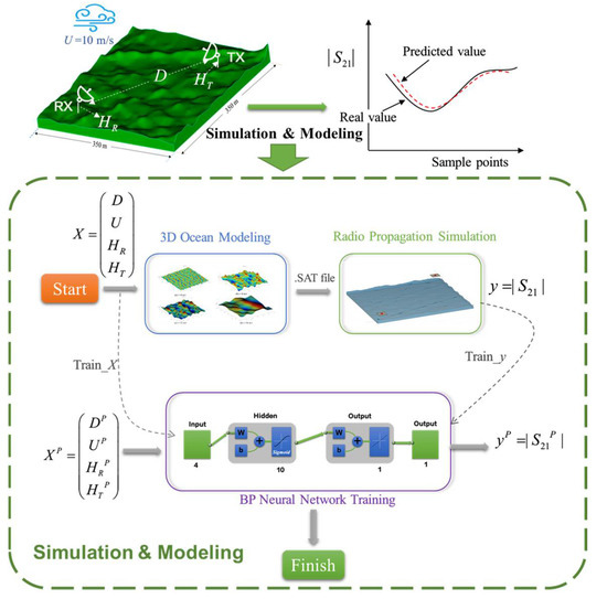
Figure 1.
The schematic illustration of the work, where D means antenna distance, HR, HT are height of receiving antenna (RX) and transmitting antenna (TX), U is wind speed, and S21 is radio propagation loss. X stands for training input; y represents training target. XP is the prediction input, yP is the prediction response.
2. Methodology
In this section, we will illustrate the realization of the simulation-training process, including 3D large-scale sea surface geometry generation, full-wave radio propagation simulation, and the neural-network-assisted surrogate model of radio propagation loss between the antennas on ships over the sea surface.
2.1. Rough Sea Surface Modeling Based on Directional Spectrum
The sea surface is a naturally formed complex and dynamic rough surface, and its formation is influenced by ocean surface wind speed, sea surge, and other factors [47]. Ocean surface wind plays a dominant role in changing the shape of the sea surface. Considering that the time scale of ocean wave movement is relatively large compared to the duration of radio wave propagation, we assume that the sea surface is static during the radio wave propagation.
Major methods for building a three-dimensional (3D) sea surface can be divided into two parts [35]. The first is based on the physical characteristics of the ocean wave such as Navier–Stokes equation. It is precise but consumes too many computational resources. The second builds a 3D sea surface through the inversion of selected ocean wave spectra. The ocean wave observation results derive the ocean wave spectrum and the Inverse Fast Fourier Transform (IFFT) converts the spectrum in the frequency domain to the 3D sea surface in space domain. To reduce the computation load, we choose the spectrum-based method, specifically, the one-dimensional Pierson–Moskowitz (P-M) spectrum [24] are combined with the direction expansion formula Stereo Wave Observation Program (SWOP) [47] to generate a 3D sea surface.
The spectrum-based method comes from linear wave theory, which is widely used in ocean engineering and computer graphics. In this approach, linear ocean waves are viewed as the superposition of harmonics with different amplitudes, phases, and directions. The ocean wave spectrum describes the distribution of these harmonics in the frequency domain. According to Fourier Transform theory, to calculate the instant height z of every certain two-dimensional point , we should use (1):
where is the initial wave height (typical value equals to 0), n represents the number of harmonic waves, stands for the amplitude of harmonic waves, and is the frequency of harmonic waves. The angular frequency . The wave number is where is the wavelength. represents the wave propagation direction in the horizontal plane, is the initial phase angle, which is generally a random quantity. The variable t stands for time.
According to the linear wave theory, for deep water waves, we have:
where g represents the gravitational acceleration, is the wave number, and is the angular frequency.
As shown in (1), the amplitude , frequency , and direction for every single harmonic wave determine the wave height. Therefore, we extract these parameters from the directional spectrum.
Assume there is a function containing the angular frequency and wave direction of the unit wave, and within the interval from to and to , the energy is proportional to . We call the direction spectrum of the ocean wave:
where is the amplitude of the harmonic wave, and and mean the ith frequency sample value and j-th wave direction sample value, respectively. and stand for the step intervals of and .
Since wave spectra are usually one-dimensional, to obtain a 2D spectrum, we will introduce the direction expansion function . After that, the 2-D spectrum can be formulated as:
In (4), is the 1D spectrum, and is the angle between the main direction of the sea wave, which is usually replaced by the average wind direction, and the wave direction of the unit wave.
We choose the P-M spectrum as in this research. The P-M spectrum is a one-dimensional spectrum proposed by Neumann and Pierson. It describes fully developed seas under certain wind influence and is derived from statistical observation in the North Atlantic. The formulation is:
where , and g stands for gravitational acceleration constant. There is only one variable parameter, , in (5), which stands for the wind speed at 10 m above sea level, indicating that the wind speed determines the energy distribution. Figure 2 illustrate the relationship between different wind speeds with the energy distribution. We can obtain that most of the energy is distributed between angular frequencies of 1 and 2 rad/s.
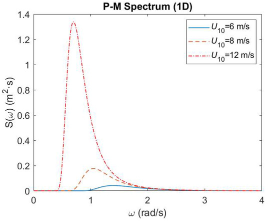
Figure 2.
Energy distribution under different wind speeds. The higher the wind speed is, the more concentrated the energy distribution.
As for direction expansion function, it must satisfy (6):
From (6), we can obtain the spectrum energy E in frequency range and the total energy of directional spectrum :
The direction spectrum employed in this research is from the Stereo Wave Observation Program, which is conducted by U. S. Navy organizations and civilian research organizations as:
where p and q are parameters related to and , which can be obtained through (10) and (11), respectively:
where .
Figure 3 illustrates the 2D wave spectrum . Since the energy is only distributed in a limited area, we can decrease the upper frequency limit in our simulation, and it will be introduced in Section 3.1.
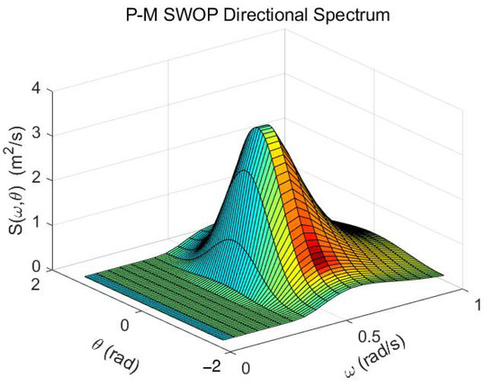
Figure 3.
The 2D PM-SWOP spectrum with the wind speed of 12 m/s. is in the range [ ].
2.2. Simulation of Radio Wave Propagation over Sea
Radio wave propagation models are generally divided into two types: experimental models and analytical models. Experimental models are established based on observation data or mathematical modeling experiments [18,19,20], while analytical models analyze the propagation mechanism of radio waves, which directly finds the main propagation routes based on phenomena such as reflection, diffraction, and scattering [10].
Aimed at simulating ship-to-ship communication, we conducted short-distance radio propagation in our research to establish an empirical–analytical combined propagation model. Considering that practical frequency in maritime communication usually ranges from 1.6 MHz to 25.6 MHz and the working frequency determines the length of the antenna [48,49,50], we set the working frequency at 5 MHz.
2.3. Surrogate Model Based on Machine Learning
In a typical surrogate model, the commercial software package CST is used as a reliable forward modeling tool which can perfectly simulate the propagation in the physical world, and then the output can be used as the truth value. We can obtain high-precision response data which are calculated by the CST and build the surrogate model between the input parameters and the output response value [51]. Figure 4 represents the most typical surrogate model generation process. The computation is completely hidden, as what we are interested in is only the input and output [52].
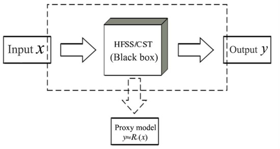
Figure 4.
The illustration of surrogate model design. The output value can be calculated by commercial software automatically.
Furthermore, as a surrogate model requires a large amount experimental data, a highly efficient batch simulation is required. In our research, we use python scripts to realize this procedure, and it will be introduced in Section 3.2.
After the training data are obtained, we establish an analytical model between the input parameter and output response. Backpropagation (BP) [53] neural network is a widely used neural network for training regression and classification tasks. In our study, we used a BP neural network to fit our radio propagation response data with input parameters and obtained the prediction model. The basic BP neural network process is described in Figure 5 [54].
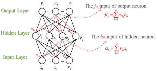
Figure 5.
BP network schematic diagram and variable in the algorithm.
Given a network with d features, l outputs, and q hidden layers, assume hidden layers and output layers use the Sigmoid function as the activate function, where represents the threshold of the jth output neuron and represents the threshold of the jth hidden neuron. The weight between the ith input neuron and hth hidden neuron is , and the weight between the hth hidden neuron and jth output neuron is . The input for the hth hidden neuron is , and the input for the jth output neuron is .
Given a training sample , assume that the truth is n-dimensional, which is . The output of the neural network is . The jth component of can be calculated through:
where f depends on the exact activation function, for example, Rectified Linear Activation Function (ReLU).
Then, the mean square error (MSE) of the network on is:
To determine the weights and threshold of the network, we should update the parameters using gradient descent strategy. The update formulation of parameter is:
where is the learning rate, is the gradient of the mean square error, and the weight value is continuously updated until the loss function reaches the stop requirement.
The gradient of the jth output layer neuron is:
and the update formula of in the BP algorithm is:
The gradient of hidden layer neurons is:
while the update formulas of in the BP algorithm are:
The learning rate controls the update step during every iteration.
In the training process, we provide an input neural layer with the training set. Then, the network will calculate the forward weight until reaching the output layer. We calculate the output error and back-propagate it to hidden layers. Finally, we will adjust the weights and the thresholds according to the hidden layer errors. The algorithm will stop until certain requirements are satisfied. Algorithm 1 describes the process of back propagation.
| Algorithm 1. Back Propagation Algorithm. | |
| Input: | Train set , learning rate |
| Procedure: | |
| 1. | Randomly initialize all connection weights and thresholds in the network within the range of (0, 1) |
| 2. | Repeat |
| 3. | for all do |
| 4. | Calculate current output |
| 5. | Calculate the gradient of the output layer neuron. |
| 6. | Calculate the gradient of hidden layer neurons |
| 7. | Update connection weight and threshold |
| 8. | end for |
| 9. | until: stop requirement satisfied |
| Output: | Multi-layer feedforward neural network with connection weights and thresholds determined |
3. Results
3.1. Three-Dimensional Sea Surface Establishment
The directional spectrum is a continuous function of frequency and direction . It must be discrete in practical calculation, and a limited number of unit waves will be sampled to synthesize the ocean waves. We defined a sampling area , and it can cover 99.9 % of the energy in the frequency domain. Both the frequency and direction interval and are divided uniformly. In this research, we set and , where N and M are the numbers of sampling frequencies and directions. We take according to (9) in this research.
As illustrated in (5), the energy is mainly distributed in the low frequency range when the wind speed is relatively high. It is important to set a proper limit to the and in integral (7) to avoid energy leakage. A large amount computing resources will be saved through accurate limit settings.
We set the upper limit of the integral (7) as , where the integration value is equal to . We calculate under different wind speeds, and the results are shown in Table 2.
Table 2.
With different wind speeds.
The relationship between windspeed and is apparently a smooth curve, as shown in Figure 6, and the regressive model is:
where U is the wind speed.
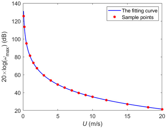
Figure 6.
Sample points are fitted by Equation (21) perfectly; is rescaled by log.
In the experiment, the wind speeds range from 2 m/s to 20 m/s, and the wind speed interval is set as 2 m/s. The size of the sea is set to be to imitate real maritime communication scenarios under small distances between ships. Figure 7 is the sample sea surface, which is utilized in our propagation simulation experiment.
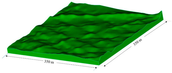
Figure 7.
The 3D ocean geometry with the size of .
Traditional 3D modeling software such as Maya, Unity, and SolidWorks do not support script operation. Coreform Cubit is a fully featured software toolkit for robust generation of two- and three-dimensional finite element meshes (grids) and geometry preparation. Scripting functionality is available directly via the command line with a built-in python interpreter or via file input for batch mode operation. In our experiment, we utilize the python API interface provided by Cubit to build the 3D ocean area automatically.
The process is indicated in Figure 8. The input parameter is only wind speed U, and the script will generate a height map based on the 3D ocean spectrum equation. Then, the Cubit API is called, the 3D surface is drawn in Cubit anonymously, and the 3D sea entity is created by “webcut” tool in this software. In the end, the sea entity is exported automatically. The script realizes an automatic method of 3D sea entity creation.
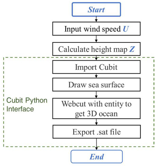
Figure 8.
Python API provided by CUBIT offers batch generation ability. In this research, the input parameter is only the wind speed vector.
Figure 9 shows the sea surface under the influence of different wind speeds. Corresponding to our prior knowledge, the faster the wind is, the choppier the sea surface is. When the wind speed is 4 m/s, the sea surface tends to be flat with small ripples.
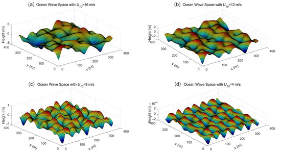
Figure 9.
The 3D sea surface simulation figure with different wind speeds of (a) U = 16 m/s; (b) U = 12 m/s; (c) U = 8 m/s; (d) U = 4 m/s.
3.2. Radio Propagation Simulation over Rough Sea
Simulation of the radio propagation is realized through commercial software CST Studio Suite (CST).
As discussed in Section 2.3, automatic batch simulation plays a key role in this research. We utilize the python API to control the CST. Simulation and data exporting are performed automatically by the python script interface. Through the script operation, we can make sure every operation in CST is standard and precise; human operation interaction will be excluded.
Figure 10 explains the procedures in the python script. The program starts with reading radio propagation parameter table, which includes ship distance and antenna height. After that, the CST python API will be called and enter the background computation mode. In this stage, the 3D sea entity is imported into the workspace and radio propagation simulation is conducted by CST microwave function. Finally, the response data and simulation project file will be saved automatically. With proper loop setting and reading result script, the Python script will form a table which includes the input sea parameters and output response data, fulfilling the automatic method of batch simulation and exportation.
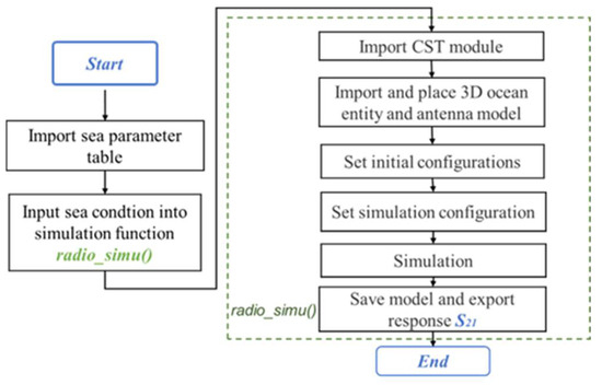
Figure 10.
The diagram for automatic batch simulations. Sea parameters including ship distance D, antenna heights HR and HT, and wind speed U are input parameters, and the response will be exported to a table automatically.
In our research, two 1/4 monopole antennas working at MHz are set up in the experiment as signal-transmitting and -receiving devices. means the wavelength of the radio signal and can be calculated through Equation (22):
where c means the speed of light.
The wind speed ranges from 1 m/s to 20 m/s. The distance between the two antennas ranges from 141 m to 500 m, and the distance between the antenna and the sea surface ranges from 6 m to 20 m.
Figure 11a shows the monopole antenna used in our research, the antenna height is 15 m, and the GND is designed as a 30 m × 30 m square. Figure 11b shows the relative position of two antenna above the sea, which is also an illustration of simulation scenery in CST.
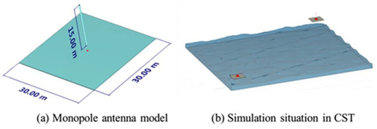
Figure 11.
Monopole antenna model and radio propagation simulation schematic diagram, where the GND is a 30 m × 30 m square, and the pole’s length equals to 15 m.
3.3. BP Neural Network Generates Prediction Model
3.3.1. Experimental Data Set
After the radio propagation simulation, we obtain the radio propagation decay ratio S21, where S21 stands for the ratio between the received signal and transmitted signal with in dB. In the large-scale experiment, we obtained 250 sets of loss data of samples points.
Some preprocessing steps are necessary on the response data. According to related surveys [22,55], when a radio propagates in close distance (<1 km), the radio wave mainly follows the double path propagation, which can be expressed as:
where HT and HR denote the heights of the transmitting antenna and the receiving antenna, and D is the antenna distance.
Therefore, we conduct the data preprocessing as , where x could be distance D or antenna heights HT and HR.
In Table 4, we list part of our training dataset, which is composed of the variables including wind speed, ship distance, antenna height, and the radio signal attenuation response S21.
In Table 3, D means antenna distance; HR, HT are the height of the receiving antenna and transmitting antenna, respectively; U is the wind speed; and S21 is the ratio between the received signal and transmitted signal in dB.
Table 3.
Partial Input Sea Parameter and Output Response.
In this study, the wind speed, the distance between the ships, and the heights of the transmitting and receiving antenna are independent variables.
3.3.2. Evaluation Criteria for Prediction Capacity
Targeting predicting propagation-loss, the Mean Square Error (MSE evaluation criterion) is proposed to optimize the prediction model. The coefficient of determination R Squared () reveals the model’s capacity.
The MSE represents the average of squared error between the predicted propagation loss value () and the real loss value ():
The R Squared represents the proportion of the variance for a dependent variable that is explained by an independent variable or variables in a regression model:
3.3.3. Other Compared Classical Machine Learning Methods
Generally speaking, our task is a typical regression problem. In the machine learning field, there already exist many mature tools to perform regression tasks, such as support vector machines (SVM), artificial neural networks (ANN), and some ensemble methods such as random forest. Considering that the size of our training dataset and the dimensions of the data are relatively small in the context of machine learning, classical machine learning methods can already make the R2 over 0.9, which means it has high credibility. To verify the effectiveness of our proposed method, we made a comparison with three other classical machine learning method, which are the support vector machine, decision tree, and random forest methods. The three methods are estimated as having good performance when handling regression problems. Other state-of-the-art machine learning or deep learning methods such as LSTM [56], ResNet [57], or Transformer [58] perform well in large datasets and complex tasks but have little contribution to the optimization of task scores on the basis of BP neural networks. In our study, we will focus on the optimization of classical regression methods.
- Support Vector Machine (SVM):
SVM is an algorithm for supervised learning, used for classification and regression. SVM’s aim is to find the individual hyperplane with the highest margin that can divide the classes linearly. The goal of supporting vector machine learning is to identify data sets where the number of training data is limited and where the optimal solution cannot be ensured by the normal use of large numbers of statistics. In order to find a hyperplane that better divides data into its groups, SVM utilizes different kernel functions such as the radial base function (RBF) or polynomial kernel and, when used for minimal training sets, has good classification performance. SVM is basically designed to solve classification problems, and the method of Support Vector Classification (SVC) can be extended to solve regression problems, which is called Support Vector Regression (SVR) [59].
- 2.
- Decision Tree (DT) method [60]:
DT is a data mining method targeting classification tasks which are based on multiple covariates. This method classifies a population into branch-like segments that construct an inverted tree with a root node, internal nodes, and leaf nodes. The algorithm is non-parametric and can efficiently deal with large, complicated datasets without imposing a complicated parametric structure. When the sample size is large enough, study data can be divided into training and validation datasets. The training dataset is used to build a decision tree model and a validation dataset to decide on the appropriate tree size needed to achieve the optimal final model.
- 3.
- Random Forest (RF) method [61]:
Random Forest Regression is a supervised learning algorithm that uses ensemble learning method for regression, classification, and other tasks. The ensemble learning method is a technique that combines predictions from multiple machine learning algorithms to make a more accurate prediction than a single model. The combination of several machine learning techniques can reduce variance and prevent overfitting, reduce bias, and improve prediction. Bagging (Bootstrap aggregating) [62], AdaBoost (Adaptive boosting) [63], and stacking are utilized here.
3.3.4. Optimization of the BP Neural Network
In our study, we proposed the BP neural network as the most advantageous method in prediction. As shown in Figure 12, the network is composed of one input layer, one hidden layer, and one fully connected layer with one dimension output. The activation function in the hidden layer is Sigmoid. We optimize the squared error MSE using the stochastic gradient method. A regularization term is added to the loss function which shrinks model parameters to prevent overfitting.
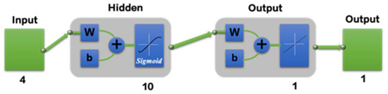
Figure 12.
BP neural network illustration with Sigmoid hidden neurons and linear output neurons.
Considering the dataset size, the maximum iteration number is set to 10,000, and the batch size is set to 64. Cross-Validation (CV) is utilized to avoid over-fitting, the number of k folds is set to 5. The ratio of training data to testing data is set to 8:2, and validation is no longer required according to CV. Early stopping is set to true to avoid over-fitting and unnecessary resource consumption.
Hyper parameter tuning is conducted under a grid search, which contains all possible parameter combinations. Hidden-layer neurons; the activation function, which contains tanh and Rectified Linear Unit (ReLU); the solver for weight optimization, which includes limited-memory BFGS (L-BFGS), Adam optimization. and Stochastic Gradient Descent (SGD); the learning rate method, which includes constant and adaptive methods; and the strength of the L2 regularization term are considered and included in the parameter search field. A standard scaler is applied before training the model to make sure that all features are centered around 0 and have variance in the same order.
The results of the tuned hyper parameters are shown in Table 4.
Table 4.
Hyper Parameter Table of Tuned BP Network.
Figure 13 shows the MSE curve during training with the tuned parameters. The training obtained the best performance at epoch 58. It is obvious that the early stopping criterion is satisfied before the max iteration. The global minimum is equal to local minimum, proving that the learning rate is properly set. The ratio of MSE between the training and test is 0.57:1, demonstrating that there is no overfitting and the neural network is well trained.
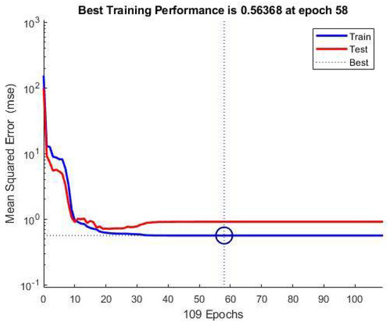
Figure 13.
Performance of the BP neural network. Validation reaches best performance at epoch 58 with an MSE value equals to 0.563.
3.3.5. Propagation Loss Result
The proposed modeling method is compared with other traditional methods such as SVM, DT, and RF. Figure 14 shows a comparison of the prediction performance of all propagation-loss prediction methods on an individual test set which contains 50 test samples. The blue line represents the truth data, the red line is our proposed method, and the green, purple, and yellow lines are the results of the SVM, decision tree, and random forest, respectively. These methods all achieve relatively high precision, providing high credibility. In qualitative analysis, these prediction models perform well when the propagation loss is between 20 dB and 35 dB. For larger or smaller truth data, the BP neural network has better results compared with the other three methods. As for further quantitative comparison, the evaluation table is introduced.
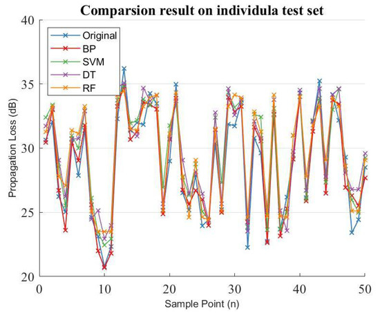
Figure 14.
Comparison results of prediction performance of all prediction approaches. The x axis means different sample, the y axis is the corresponding propagation loss.
As we can see in Table 5, the evaluation index results of the different prediction models shows that the proposed and tuned network owns the best prediction capacity at R2 equals to 0.9250 and the MSE is only 1.2146.
Table 5.
Evaluation Result of Predictive Capacity.
4. Discussion
Overall, our study established an automatic and convenient way for radio propagation loss prediction. The previous analytical model for loss prediction requires precise observation data and has limitations for antennas’ working frequency range and applicable propagation distance range. The loss prediction model established through our method is not limited by the applied frequency range or distance range as we can adjust our working frequency and sea size in simulation. Furthermore, our approach fills in the blanks of the data end in traditional prediction model establishment. Through the efforts of automatic batch simulation, we could obtain radio propagation loss data of both high credibility and large quantity. The full simulation requires only the computation resources, so the expenses of outdoor long-time observation are not necessary anymore, which greatly saves funds.
A summary of the computation time for the simulation process of the rough sea radio propagation is shown in Table 6. The Full Wave Simulation contains sea surface generation and radio propagation simulation. Usually it costs more than 2 h to obtain the target radio signal attenuation data; however, once the neural network prediction model is well trained, the time for prediction response time decreases greatly from 2 h to 0.2 s while still keeping high credibility.
Table 6.
Computation Time for Simulation and Prediction.
However, in our study, the input propagation loss data are limited as the simulation output does not contain the data obtained from on-site observations. We found that public over sea radio propagation loss datasets are rare and usually do not meet our requirements, for example, the dimensions of the variables and the number of training samples. We would like to cooperate with other laborites that own such data and implement them in our further work.
The comparison between traditional prediction models such as Longley–Rice and our neural network predictor should also be conducted. However, due to limits of appliable working frequencies and distance ranges, the traditional prediction models do not fit our simulation data, and we could not continue on it. We would like to change our simulation environment and introduce it in a future work.
5. Conclusions
In this paper, we proposed a new approach to automatically build an empirical–analytical maritime radio propagation loss model. First, we build 3D oceans through spectrum theory, and then simulation of radio propagation over the 3D ocean is conducted by software to obtain the propagation loss. The first two steps are conducted by a python script automatically. Finally, we utilize a BP network to fit the output propagation loss with input parameters. The well-trained BP network can perform predictions effectively on independent data sets which are not included in the training process.
In this model, the influence of the irregular sea surface, which is represented by windspeed, U, is taken into consideration. Compared with other traditional methods, the proposed model is more precise when predicting over sea radio propagation. Furthermore, the propagation loss prediction model can automatically provide real time prediction and adjust input parameters in case of sudden weather changes, which are really common over the ocean.
Our study fills in the blanks for automatic over sea radio signal propagation simulation and breaks the limits for the appliable distance range and working frequency, making it adaptive for different tasks.
Author Contributions
Conceptualization, W.Z. and Q.R.; methodology, W.Z. and S.S.; software, S.S. and Y.L.; validation, S.S., X.Z. and H.Z.; formal analysis, S.S. and W.Z.; investigation, S.S. and H.Z.; resources, W.Z. and Q.R.; data curation, H.Z., X.Z. and Y.L.; writing—original draft preparation, S.S.; writing—review and editing, W.Z. and Q.R.; visualization, H.Z.; supervision, W.Z. and Q.R.; project administration, W.Z.; funding acquisition, W.Z. All authors have read and agreed to the published version of the manuscript.
Funding
This research was funded by the National Natural Science Foundation of China, grant number 92166107 and 61801009.
Data Availability Statement
The simulated radio propagation data and machine learning codes are available at https://github.com/shengfus/Maritime_Radio_Propagation (accessed on 1 July 2022).
Conflicts of Interest
The authors declare no conflict of interest. The funders had no role in the design of the study; in the collection, analyses, or interpretation of data; in the writing of the manuscript, or in the decision to publish the results.
References
- Uribe, C.; Grote, W. Radio Communication Model for Underwater WSN. In Proceedings of the 2009 3rd International Conference on New Technologies, Mobility and Security, Cairo, Egypt, 23 December 2009; IEEE: Cairo, Egypt, 2009; pp. 1–5. [Google Scholar]
- Jimenez, E.; Quintana, G.; Mena, P.; Dorta, P.; Perez-Alvarez, I.; Zazo, S.; Perez, M.; Quevedo, E. Investigation on Radio Wave Propagation in Shallow Seawater: Simulations and Measurements. In Proceedings of the 2016 IEEE Third Underwater Communications and Networking Conference (UComms), Lerici, Italy, 30 August–1 September 2016; IEEE: Lerici, Italy, 2016; pp. 1–5. [Google Scholar]
- Goh, J.H.; Shaw, A.; Al-Shamma’a, A.I. Underwater Wireless Communication System. J. Phys. Conf. Ser. 2009, 178, 012029. [Google Scholar] [CrossRef]
- Shaw, A.; Al-Shamma’a, A.i.; Wylie, S.R.; Toal, D. Experimental Investigations of Electromagnetic Wave Propagation in Seawater. In Proceedings of the 2006 European Microwave Conference, Manchester, UK, 10–15 September 2006; IEEE: Manchester, UK, 2006; pp. 572–575. [Google Scholar]
- Al-Shamma’a, A.I.; Shaw, A.; Saman, S. Propagation of Electromagnetic Waves at MHz Frequencies Through Seawater. IEEE Trans. Antennas Propagat. 2004, 52, 2843–2849. [Google Scholar] [CrossRef]
- Hunt, K.P.; Niemeier, J.J.; Kruger, A. RF Communications in Underwater Wireless Sensor Networks. In Proceedings of the 2010 IEEE International Conference on Electro/Information Technology, Normal, IL, USA, 20–22 May 2010; IEEE: Normal, IL, USA, 2010; pp. 1–6. [Google Scholar]
- Button, R.; Acquisition and Technology Policy Center (Eds.) A Survey of Missions for Unmanned Undersea Vehicles; RAND Corporation monograph series; RAND: Santa Monica, CA, USA, 2009; ISBN 978-0-8330-4688-8. [Google Scholar]
- Zhang, J.P.; Wu, Z.-S.; Zhao, Z.-W.; Zhang, Y.-S.; Wang, B. Propagation modeling of ocean-scattered low-elevation GPS signals for maritime tropospheric duct inversion. Chin. Phys. B 2012, 21, 109202. [Google Scholar] [CrossRef]
- Ge, Y.; Kong, P.Y.; Tham, C.K.; Pathmasuntharam, J.S. Connectivity and Route Analysis for a Maritime Communication Network. In Proceedings of the 2007 6th International Conference on Information, Communications & Signal Processing, Singapore, 10–13 December 2007; IEEE: Singapore, 2007; pp. 1–5. [Google Scholar]
- Wang, J.; Zhou, H.; Li, Y.; Sun, Q.; Wu, Y.; Jin, S.; Quek, T.Q.S.; Xu, C. Wireless Channel Models for Maritime Communications. IEEE Access 2018, 6, 68070–68088. [Google Scholar] [CrossRef]
- Rappaport, T.S. Wireless Communications: Principles and Practice; Prentice Hall: Upper Saddle River, NJ, USA, 1996; ISBN 978-0-7803-1167-1. [Google Scholar]
- Durand, J.C.; Granier, P. Radar coverage assessment in nonstandard and ducting conditions: A geometrical optics approach. In IEE Proceedings F (Radar and Signal Processing); IET Digital Library: Wales and Scotland, UK, 1990; pp. 95–101. [Google Scholar]
- Popov, A.V.; Kopeikin, V.V. Electromagnetic Pulse Propagation over Nonuniform Earth Surface: Numerical Simulation. arXiv 2007. [Google Scholar] [CrossRef]
- Yang, K.; Molisch, A.F.; Ekman, T.; Roste, T. A Deterministic Round Earth Loss Model for Open-Sea Radio Propagation. In Proceedings of the 2013 IEEE 77th Vehicular Technology Conference (VTC Spring), Dresden, Germany, 2–5 June 2013; IEEE: Dresden, Germany, 2013; pp. 1–5. [Google Scholar]
- Yang, K.; Molisch, A.F.; Ekman, T.; Roste, T.; Berbineau, M. A Round Earth Loss Model and Small-Scale Channel Properties for Open-Sea Radio Propagation. IEEE Trans. Veh. Technol. 2019, 68, 8449–8460. [Google Scholar] [CrossRef]
- Doerry, A. Earth Curvature and Atmospheric Refraction Effects on Radar Signal Propagation; Sandia National Lab.: Albuquerque, NM, USA, 2013; p. 1088060. [Google Scholar]
- Gunashekar, S.D.; Siddle, D.R.; Warrington, E.M. Transhorizon Radiowave Propagation Due to Evaporation Ducting: The Effect of Tropospheric Weather Conditions on VHF and UHF Radio Paths over the Sea. Reson 2006, 11, 51–62. [Google Scholar] [CrossRef]
- Hata, M. Empirical Formula for Propagation Loss in Land Mobile Radio Services. IEEE Trans. Veh. Technol. 1980, 29, 317–325. [Google Scholar] [CrossRef]
- Medeisis, A.; Kajackas, A. On the Use of the Universal Okumura-Hata Propagation Prediction Model in Rural Areas. In Proceedings of the VTC2000-Spring. 2000 IEEE 51st Vehicular Technology Conference Proceedings (Cat. No.00CH37026), Tokyo, Japan, 15–18 May 2000; IEEE: Tokyo, Japan, 2000; Volume 3, pp. 1815–1818. [Google Scholar]
- Isabona, J.; Imoize, A.L. Terrain-Based Adaption of Propagation Model Loss Parameters Using Non-Linear Square Regression. J. Eng. Appl. Sci. 2021, 68, 33. [Google Scholar] [CrossRef]
- Kasampalis, S.; Lazaridis, P.I.; Zaharis, Z.D.; Bizopoulos, A.; Paunovska, L.; Zettas, S.; Glover, I.A.; Drogoudis, D.; Cosmas, J. Longley-Rice Model Prediction Inaccuracies in the UHF and VHF TV Bands in Mountainous Terrain. In Proceedings of the 2015 IEEE International Symposium on Broadband Multimedia Systems and Broadcasting, Ghent, Belgium, 17–19 June 2015; IEEE: Ghent, Belgium, 2015; pp. 1–5. [Google Scholar]
- Kasampalis, S.; Lazaridis, P.I.; Zaharis, Z.D.; Bizopoulos, A.; Zettas, S.; Cosmas, J. Comparison of Longley-Rice, ITU-R P.1546 and Hata-Davidson Propagation Models for DVB-T Coverage Prediction. In Proceedings of the 2014 IEEE International Symposium on Broadband Multimedia Systems and Broadcasting, Beijing, China, 25–27 June 2014; IEEE: Beijing, China, 2014; pp. 1–4. [Google Scholar]
- Ying, Q.; Zhou, Y. Research on Electromagnetic Wave Propagation Model of Sea Area. Master’s Thesis, Hainan University, Haikou, China, 2015. [Google Scholar]
- Teixeira, P.R.F.; Davyt, D.P.; Didier, E.; Ramalhais, R. Numerical Simulation of an Oscillating Water Column Device Using a Code Based on Navier–Stokes Equations. Energy 2013, 61, 513–530. [Google Scholar] [CrossRef]
- Pozzer, C.T.; Pellegrino, S.R.M. Procedural Solid-Space Techniques for Modeling and Animating Waves. Comput. Graph. 2002, 26, 877–885. [Google Scholar] [CrossRef]
- Alves, J.H.G.M.; Banner, M.L.; Young, I.R. Revisiting the Pierson–Moskowitz Asymptotic Limits for Fully Developed Wind Waves. J. Phys. Oceanogr. 2003, 33, 1301–1323. [Google Scholar] [CrossRef]
- Longuet-Higgins, H.C. A Computer Algorithm for Reconstructing a Scene from Two Projections. Nature 1981, 293, 133–135. [Google Scholar] [CrossRef]
- Joelson, M.; Ramamonjiarisoa, A. A Non-Linear Second-Order Stochastic Model of Ocean Surface Waves. Oceanol. Acta 2001, 24, 409–415. [Google Scholar] [CrossRef]
- Jensen, L.S.; Golias, R. Deep-Water Animation and Rendering. In Proceedings of the Game Developer’s Conference (Gamasutra), San Francisco, CA, USA, 10–12 October 2001. [Google Scholar]
- Tessendorf, J.; others Simulating Ocean Water. Simulating nature: Realistic and interactive techniques. Siggraph 2001, 1, 5. [Google Scholar]
- Fréchot, J. Realistic Simulation of Ocean Surface Using Wave Spectra. In Proceedings of the First International Conference on Computer Graphics Theory and Applications (GRAPP 2006), Setúbal, Portugal, 25–28 February 2006; pp. 76–83. [Google Scholar]
- Chen, L.; Shaogui, D.; Zhiqiang, L.; Yiren, F.; Jingjing, Z.; Jutao, Y. Simulation and Application of Electromagnetic Wave Propagation Logging Tool in Microwave Band Based on CST. In Proceedings of the 2021 13th International Symposium on Antennas, Propagation and EM Theory (ISAPE), Zhuhai, China, 1–4 December 2021; IEEE: Zhuhai, China, 2021; pp. 1–3. [Google Scholar]
- Cao, T.; An, C.; Tian, Y. Study on Electromagnetic Propagation Characteristics of Two-Layer Media with CST Software; AIP Publishing LLC: Chongqing, China, 2017; p. 020021. [Google Scholar]
- Seretis, A.; Sarris, C.D. An Overview of Machine Learning Techniques for Radiowave Propagation Modeling. IEEE Trans. Antennas Propagat. 2022, 70, 3970–3985. [Google Scholar] [CrossRef]
- Zhang, G.; Patuwo, B.E.; Hu, M.Y. Forecasting with artificial neural networks: The state of the art. Int. J. Forecast. 1998, 14, 35–62. [Google Scholar] [CrossRef]
- Stocker, K.E.; Landstorfer, F.M. Empirical Prediction of Radiowave Propagation by Neural Network Simulator. Electron. Lett. 1992, 28, 724. [Google Scholar] [CrossRef]
- Popescu, I.; Nikitopoulos, D.; Constantinou, P.; Nafornita, I. ANN Prediction Models for Outdoor Environment. In Proceedings of the 2006 IEEE 17th International Symposium on Personal, Indoor and Mobile Radio Communications, Helsinki, Finland, 11–14 September 2006; IEEE: Helsinki, Finland, 2006; pp. 1–5. [Google Scholar]
- Stankovic, Z.; Milovanvic, B.; Veljkovic, M.; Dordevic, A. The Hybrid-Neural Empirical Model for the Electromagnetic Field Level Prediction in Urban Environments. In Proceedings of the 7th Seminar on Neural Network Applications in Electrical Engineering, 2004, NEUREL 2004, Belgrade, Serbia, 23–25 September 2004; IEEE: Belgrade, Serbia, 2004; pp. 189–192. [Google Scholar]
- Neskovic, A.; Neskovic, N.; Paunovic, D. Indoor Electric Field Level Prediction Model Based on the Artificial Neural Networks. IEEE Commun. Lett. 2000, 4, 190–192. [Google Scholar] [CrossRef]
- Mom, J.M.; Mgbe, C.O.; Igwue, G.A. Igwue. Application of artificial neural network for path loss prediction in urban macrocellular environment. Am. J. Eng. Res. 2014, 3, 270–275. [Google Scholar]
- Ostlin, E.; Zepernick, H.-J.; Suzuki, H. Macrocell Path-Loss Prediction Using Artificial Neural Networks. IEEE Trans. Veh. Technol. 2010, 59, 2735–2747. [Google Scholar] [CrossRef]
- Cheerla, S.; Ratnam, D.V.; Borra, H.S. Neural Network-Based Path Loss Model for Cellular Mobile Networks at 800 and 1800 MHz Bands. AEU Int. J. Electron. Commun. 2018, 94, 179–186. [Google Scholar] [CrossRef]
- Dang, M.; Wu, J.; Cui, S.; Guo, X.; Cao, Y.; Wei, H.; Wu, Z. Multiscale Decomposition Prediction of Propagation Loss in Oceanic Tropospheric Ducts. Remote Sens. 2021, 13, 1173. [Google Scholar] [CrossRef]
- Nagao, T.; Hayashi, T. Study on Radio Propagation Prediction by Machine Learning Using Urban Structure Maps. In Proceedings of the 2020 14th European Conference on Antennas and Propagation (EuCAP), Copenhagen, Denmark, 15–20 March 2020; IEEE: Copenhagen, Denmark, 2020; pp. 1–5. [Google Scholar]
- Wu, L.; He, D.; Ai, B.; Wang, J.; Qi, H.; Guan, K.; Zhong, Z. Artificial Neural Network Based Path Loss Prediction for Wireless Communication Network. IEEE Access 2020, 8, 199523–199538. [Google Scholar] [CrossRef]
- Imai, T.; Kitao, K.; Inomata, M. Radio Propagation Prediction Model Using Convolutional Neural Networks by Deep Learning. In Proceedings of the 2019 13th European Conference on Antennas and Propagation (EuCAP), Krakow, Poland, 31 March–5 April 2019; pp. 1–5. [Google Scholar]
- Li, Z.Y.; Hou, X.L. Ocean Wave Real-Time Simulation Based-on Ocean Wave Spectrum and FFT. AMR 2014, 926–930, 3531–3536. [Google Scholar] [CrossRef]
- Best, S.R. On the Use of Scale Brass Models in HF Shipboard Communication Antenna Design. IEEE Antennas Propag. Mag. 2002, 44, 12–23. [Google Scholar] [CrossRef]
- Baldwin, P.J.; Boswell, A.G.P.; Brewster, D.C.; Allwright, J.S. Iterative Calculation of Ship-Borne HF Antenna Performance. IEE Proc. H Microw. Antennas Propag. 1991, 138, 151. [Google Scholar] [CrossRef][Green Version]
- Baker, J.; Youn, H.-S.; Celik, N.; Iskander, M.F. Low-Profile Multifrequency HF Antenna Design for Coastal Radar Applications. Antennas Wirel. Propag. Lett. 2010, 9, 1119–1122. [Google Scholar] [CrossRef]
- Bandler, J.W.; Biernacki, R.M.; Chen, S.H.; Grobelny, P.A.; Hemmers, R.H. Space Mapping Technique for Electromagnetic Optimization. IEEE Trans. Microw. Theory Tech. 1994, 42, 2536–2544. [Google Scholar] [CrossRef]
- Zeng, F.; Duan, B. An Adaptive Metamodel and Its Application on Integrated Electromechanical Optimization of Reflector Antennas. Master’s Thesis, Xidian University, Xi’an, China, 2015. [Google Scholar]
- Li, J.; Cheng, J.; Shi, J.; Huang, F. Brief Introduction of Back Propagation (BP) Neural Network Algorithm and Its Improvement. In Advances in Computer Science and Information Engineering; Jin, D., Lin, S., Eds.; Springer: Berlin/Heidelberg, Germany, 2012; pp. 553–558. [Google Scholar]
- Zhou, Z.-H. Machine Learning; Springer Nature: Berlin, Germany, 2021. [Google Scholar]
- Wang, Z.; Fan, W.; Lin, M. Study and simulation on sea-surface propagation prediction model. Chin. J. Radio Sci. 2008, 23, 1095–1099. [Google Scholar]
- Yu, Y.; Si, X.; Hu, C.; Zhang, J. A Review of Recurrent Neural Networks: LSTM Cells and Network Architectures. Neural Comput. 2019, 31, 1235–1270. [Google Scholar] [CrossRef] [PubMed]
- He, K.; Zhang, X.; Ren, S.; Sun, J. Deep Residual Learning for Image Recognition. In Proceedings of the IEEE Conference on Computer Vision and Pattern Recognition, Las Vegas, NV, USA, 27–30 June 2016; pp. 770–778. [Google Scholar]
- Vaswani, A.; Shazeer, N.; Parmar, N.; Uszkoreit, J.; Jones, L.; Gomez, A.N.; Kaiser, L.; Polosukhin, I. Attention Is All You Need. In Proceedings of the 31st International Conference on Neural Information Processing Systems, Long Beach, CA, USA, 4–9 December 2017; Curran Associates Inc.: Red Hook, NY, USA, 2017; pp. 6000–6010. [Google Scholar]
- Abdullah, D.M.; Abdulazeez, A.M. Machine Learning Applications Based on SVM Classification A Review. Qubahan Acad. J. 2021, 1, 81–90. [Google Scholar] [CrossRef]
- Song, Y.-Y.; Ying, L. Decision Tree Methods: Applications for Classification and Prediction. Shanghai Arch. Psychiatry 2015, 27, 130. [Google Scholar] [PubMed]
- Belgiu, M.; Drăguţ, L. Random Forest in Remote Sensing: A Review of Applications and Future Directions. ISPRS J. Photogramm. Remote Sens. 2016, 114, 24–31. [Google Scholar] [CrossRef]
- Breiman, L. Bagging Predictors. Mach. Learn. 1996, 24, 123–140. [Google Scholar] [CrossRef]
- Hastie, T.; Rosset, S.; Zhu, J.; Zou, H. Multi-Class Adaboost. Stat. Its Interface 2009, 2, 349–360. [Google Scholar] [CrossRef]


Publisher’s Note: MDPI stays neutral with regard to jurisdictional claims in published maps and institutional affiliations. |
© 2022 by the authors. Licensee MDPI, Basel, Switzerland. This article is an open access article distributed under the terms and conditions of the Creative Commons Attribution (CC BY) license (https://creativecommons.org/licenses/by/4.0/).