A Dual-Encoder-Condensed Convolution Method for High-Precision Indoor Positioning

Abstract

We study the problem of indoor positioning, which is a fundamental service in managing and analyzing objects in indoor environments. Unpredictable signal interference sources increase the degeneration of the accuracy and robustness of existing solutions. Deep learning approaches have recently been widely studied to overcome these challenges and attain better performance. In this paper, we aim to develop efficient algorithms, such as the dual-encoder-condensed convolution (DECC) method, which can achieve high-precision positioning for indoor services. In particular, firstly, we develop a convolutional module to add the original channel state information to the location information. Secondly, to explore channel differences between different antennas, we adopt a dual-encoder stacking mechanism for parallel calculation. Thirdly, we develop two different convolution kernels to speed up convergence. Performance studies on the indoor scenario and the urban canyon scenario datasets demonstrate the efficiency and effectiveness of our new approach.

1. Introduction

With the rapid development of the Internet of Things (IoT) and 5G, high-precision positioning has attracted much attention because of its widespread location-based services (LBS). Although the space-based global positioning system (GPS) has been widely used for high accuracy in outdoor scenarios, it is difficult to apply the common GPS-based localization system for indoor positioning systems because of the dependence on the line-of-sight (LOS) communication of radio signals [1]. High-precision positioning in urban canyons and indoor scenarios still face enormous challenges due to their complex environments with varying shapes and moving objects [2]. Recently, significant research efforts have been devoted to indoor positioning.

Indoor positioning plays an important role in various LBS applications, such as emergency personal navigation [3], context awareness [4], health monitoring [5], indoor parking lots [6], and smart homes [7]. Wi-Fi [8], Bluetooth [9], ultra-wideband (UWB) systems [10], radio-frequency identification tags (RFID), and other technologies have been widely adopted for indoor positioning. In addition, typical ranging techniques based on time of arrival (ToA) [11], time of flight (ToF) [12], and time difference of arrival (TDoA) [13] have been proposed which utilize time ranging and signal information among base stations. In addition, angle of arrival (AoA) [14] and angle of departure (AoD) [15] adopt the positioning principle based on phase angle measurement to calculate the arrival angle of signals by using phase difference on different array elements, which further improve the positioning accuracy of close distance. Traditional indoor positioning techniques are highly dependent on high-precision time synchronization between base stations, and are often susceptible to non-line-of-sight (NLOS) errors, which makes it difficult to further improve the positioning accuracy.

In recent years, the development of machine learning (ML) technology has brought new inspiration to many applications, such as face recognition, image processing, recommendation systems, speech recognition, and so on. Many traditional domains have been revolutionized by the embedding of deep learning (DL). For example, thanks to the advent of RCNN, end-to-end object detection can reach speeds of more than 20 FPS on 1080Ti GPU [16]. Furthermore, the learning-based cost estimators can replace traditional cost estimators in the database community [17]. It was natural to think about how to maximize the use of deep learning to design a high-precision positioning model to achieve the same improvement effect. However, high-precision positioning depends on feature mapping from the amplitude, power, and channel difference of channel state information (CSI), which means that the typical DL model cannot be directly used in high-precision positioning. For example, although both the ResNet18 [18] and GoogLeNet [19] models can achieve sub-meter accuracy, two issues remain: (1) the unique characteristics of the localization data, such as channel differences and feature mapping disconnection caused by noise, are not fully considered; (2) large network scale and a long training time mean that it is difficult to use these models to carry out practical applications [20]. To overcome the above drawbacks, Gao et al. [20] proposed a novel deep learning model, named MPRI, inspired by the convolutional neural network Inception [21], which brought the average error of positioning precision to 0.28 m in indoor environments. Sanam et al. [22] adopted the orthogonal frequency division multiplexing (OFDM) multiple-input and -output techniques to select appropriate input characteristics from the channel response by eliminating the effects of multipath subcarriers. Then, high-precision positioning was achieved by using support vector machine (SVM)-based machine learning positioning prediction. However, the existing deep learning models still face the following challenges in the application of high-precision positioning:

• The data dimension gap between different datasets is large, and the prediction needs to modify the model structure. However, simple dimensional changes can lead to missing features.
• Since the necessary location information is not embedded, the feature information of CSI is not enough to be the input of the deep learning model.
• Existing work does not consider the global feature interaction between different antennas.
• Different channel differential extractors are executed in parallel, which affects the convergence speed of the model.

In this paper, we aim to develop an efficient method, dual-encoder-condensed convolution (DECC), to enhance the positioning accuracy and to reduce the time overheads of indoor positioning problems. Firstly, we design a layer of a convolutional neural network to align the size of the CSI; then, we embed the positional encoding matrix to enrich the position features. Secondly, in the middle of the proposed model, we design a novel encoder structure to perform a multi-head dot product operation on the combined CSI feature matrix to obtain the mutual information between antennas in multiple CSI features. Finally, we develop a convolution block with two convolution kernels of different sizes for serial feature extraction of CSI feature matrices. Our main contributions are summarized as follows.

• We developed a Conv-for-Origin structure. It adopts a layer of multichannel convolutional neural network and positional encoding matrix to align the size of the original CSI matrix and embed position information between different sub-features, which could solve the problem of size inconsistency and lack of position information between different sub-feature datasets.
• We propose a novel network architecture, the dual-encoder structure. It adopts two encoder structures to calculate the dot product of CSI features through Conv-for-Origin with different weights, and obtains the mutual information between different antennas in CSI features. Furthermore, due to the existence of multiple attention, the encoder can automatically delineate the molecular space to improve the richness of CSI features.
• We propose a dual-encoder structure. It adopts two convolution kernels of different sizes to fully extract the CSI feature information. The larger one is responsible for extracting the mixed channel differences, and the smaller one is responsible for extracting the local features of the antennas and stacking them in sequence, thereby improving the positioning accuracy. Because the two different convolutions are performed in the same horizontal direction, the convergence rate of the model is very fast.

We conduct extensive empirical studies in the indoor scenarios and urban canyon scenarios in Section 4. The results show that (1) our proposed method significantly improves the positioning accuracy error; (2) the DECC approach achieves a lower time overheads and a stronger robustness in terms of signal-to-noise ratio (SNR) and data scalability. We analyze the feasibility of using this model in real time and show a feasible scheme in Section 5.

The rest of the paper is organized as follows. A brief overview of the related work is given in Section 2. Section 3 presents our proposed approachDECC. Section 4 presents our experimental results, and Section 5 finally concludes the paper.

2. Related Work

In the following, we review two main methods for high-precision indoor positioning: traditional high-precision indoor positioning methods and ML-based high-precision indoor positioning methods. Then, we present a brief description of the vision transformer.

2.1. Traditional High-Precision Indoor Positioning

Chen et al. [10] made use of the error reduced by TDOA compared with TOA to initially improve the accuracy, and at the same time used the positioning results of TOA to exclude the virtual anchor points in TDOA, thus realizing a positioning method combining TOA and TDOA. The idea of secondary clustering is used to optimize the selection of base stations to further improve the positioning accuracy. However, its positioning accuracy is limited, and the average error is only 1.717 m. Deng et al. [23] have eliminated the interference of the same frequency caused by the same frequency networking in the data transmission of positioning, and carried out the same frequency co-load of the positioning signal and the communication signal, which can achieve a higher positioning accuracy under the simulation. However, it has not been written into the 5G standard, so it is difficult to carry out large-scale promotion in real applications. The Ubisense positioning system [24] is a positioning technology that can integrate TDOA and AOA for integrated positioning, and it has the ability of direction finding to estimate the azimuth and pitch angle that other similar UWB systems do not have, which enables it to obtain a high positioning accuracy. In an environment where ultra-wideband (UWB) radio propagation is disturbed, its positioning accuracy and outliers will be greatly affected [25]. Sangthong et al. [26] propose an RSSI-based weighting Algorithm to evaluate the wireless sensor network technology for the indoor localization. Specifically, they estimate the target position from two aspects: the weight range localizer and relative span exponential weight range localizer. In this way, they significantly improve the accuracy of indoor positioning. Yang et al. [27] detail the reason that RSSI-based methods will fail in complex situations to layer power feature and channel response. They also present a deep study on their techniques, which involve resorting to finer-grained wireless channel measurements.

2.2. ML-Based High-Precision Indoor Positioning

Wang et al. [28] proposed an indoor fingerprinting system based on calibrated channel state information (CSI). The raw-phase information is extracted from the multiple antennas and subcarriers of the network interface card, and then the phase information is further compressed by a linear transformation. In the offline phase, a deep network with three hidden layers is designed to train the data, and a greedy learning algorithm is introduced to reduce the computational complexity. In the online stage, the probability method based on radial basis function is used to estimate the online position, and good performance is achieved. Gao et al. [20] proposed a two-stage neural network to extract features from the acquired data according to the information obtained by different base stations, with a precision of 0.28 m and a mean square error of 0.30. However, in the design stage of the network, the interaction information between each base station was not considered, but the individual information of each base station was modeled separately and then superimposed, which failed to capture the nonlinear relationship between the data of each base station. It is difficult to improve the accuracy further. In the lower part of the model, the speed of convergence suffers due to the two channels, and a superposition operation is performed during the convergence. Additionally, because the network depth is too large (63 layers), it takes nearly seven hours of training time and the time cost is too high. Dayekh et al. [29] utilized the diversity of channel impulse responses collected by multiple access points, and combined artificial neural networks with traditional positioning technologies such as received signal strength (RSS) and AOA for co-location, thereby improving the accuracy of traditional positioning techniques. Sanam et al. [22] proposed a free positioning technology device based on machine learning. It removes the sub-carrier noise affected by multipath, selects the most reliable localization features from the channel response, and uses support vector machines (SVM) for identification; this results in a better positioning accuracy, even in the presence of passive devices.

2.3. Vision Transformer and Convolutional Neural Network

In the deep learning community, there many studies evaluating convolutional neural networks (CNN). He et al. [18] used the residual connection to enable the network to reach hundreds of layers deep. Krizhevsky et al. [30] used the 11 × 11, 7 × 7, and 5 × 5 kernels to obtain the larger receptive field so the network can gain more prior feature. Simonyan et al. [31] replaced the large kernels by successive 3 × 3 kernels, and demonstrated that multiple nonlinear layers can increase the depth of the network to ensure the learning of more complex patterns. As VisionTransformer (ViT) has achieved remarkable results in various fields, some works attempted to combine ViT and CNN, e.g., [32,33,34,35]; these works either embedded between transformer blocks or intertwined the convolution into each transformer block. Differently from the abovementioned works, in this paper, we utilize a novel approach rather than a mixed approach. It is worth noting that, in the computer vision domain, there are millions of images available for training the model. However, when focusing on the field of high-precision indoor positioning, it is almost impossible to have that many samples for training the model. So, we need to take full advantage of the fast convergence characteristics of CNN for efficient training. Figure 1 shows the two different approaches.

3. Methodology

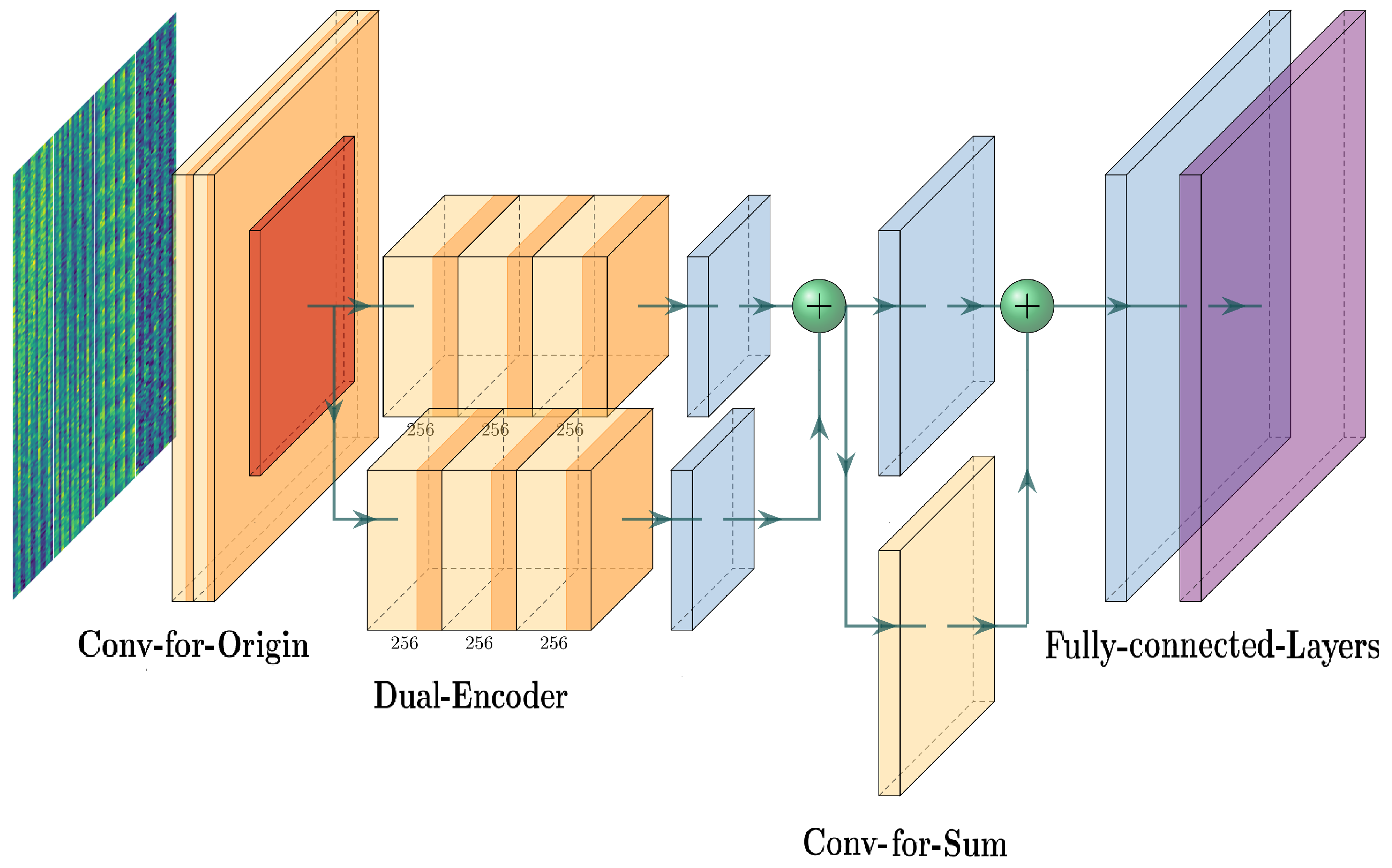
In this section, we propose a deep learning network structure—named the dual-encoder-condensed convolution (DECC) method—to improve positioning accuracy. An overview of the DECC network is illustrated in Figure 2. The proposed structure is composed of three modules: the Conv-for-Origin module, the Dual-Encoder module, and the Conv-for-Sum module. The Conv-for-Origin module is responsible for resizing the original CSI matrix and embedding the position information. The Dual-Encoder module is responsible for feature interaction of the CSI matrix, and enriches the features through the Conv-for-Origin module. The Conv-for-Sum module works for the convergence of feature information processed by different convolution kernels.

3.1. Design of the Conv-for-Origin Module

The purpose of the Conv-for-Origin layer is to embed the position information in the original CSI, to ensure the richness of the features. At the same time, the size of the original CSI matrix can be adjusted to fit the input of the later Dual-Encoder module. The data size is fixed to reduce the feature loss of the data source. Therefore, we align dimensions of the original CSI matrix using convolutional layers. This avoids the loss of features caused by simple size splicing and stacking directly on the source data. After that, the new CSI matrix can be used to obtain the position feature matrix through absolute position encoding, and the obtained position feature matrix can be superimposed with the new CSI matrix, and finally the output of the Conv-for-Origin module can be obtained. Additional design details of the Conv-for-Origin module are presented in the following subsection.

3.1.1. Original Embedding

In this module, we encode the raw CSI using a convolutional neural network. The input channel is the dimensions of the original CSI matrix, and the output channel is 400. For CSIs with different signal-to-noise ratios, the number of antennas is the same, so we share the keyword embedding convolutional neural network. Before the Dual-Encoder module, we expand the dimension of the resulting matrix, so the channels starting at 400 become $20\times 20$. For the convolutional neural network, we utilize a convolution kernel of $4\times 4$, which is larger than the common size, $5\times 5$, so it can preliminarily extract the feature information and channel differences in longitudinal antennas in CSI.

3.1.2. Positional Embedding

After the above convolutional neural network, the original CSI sequence is completely disrupted, and the subsequent self-attention dot product operation does not consider the position information between features. To obtain the position information of different antenna sub-features in the CSI matrix, we add position embedding to the module, and use the trigonometric function to output a position-encoding matrix with the same size as the CSI matrix. We add the obtained position code matrix with the CSI matrix, so that the CSI can obtain rich positional information. There are many options for positional encoding sequences, some are learned and some are fixed [36]. The formula of the position encoding we used is as follows:

$$P{E}_{(pos,2i)}=sin(pos/{\mathrm{10,000}}^{2i/d_{model}})$$

(1)

$$P{E}_{(pos,2i+1)}=cos(pos/{\mathrm{10,000}}^{2i/d_{model}})$$

(2)

where $d_{model}$ is the dimension of the CSI matrix, $pos$ is the position of the sub-feature, and i represents the dimension. The output of the Conv-for-Origin module consists of two parts. We compute the output matrix as:

$$\mathtt{Conv}-\mathtt{for}-\mathtt{Origin}\left(x\right)=conv\left(x\right)+pos\left(conv\right(x\left)\right)$$

(3)

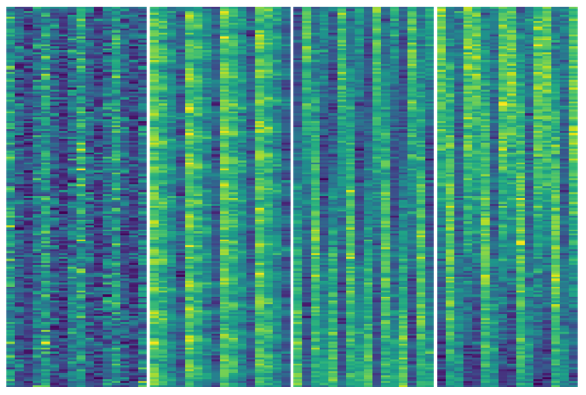
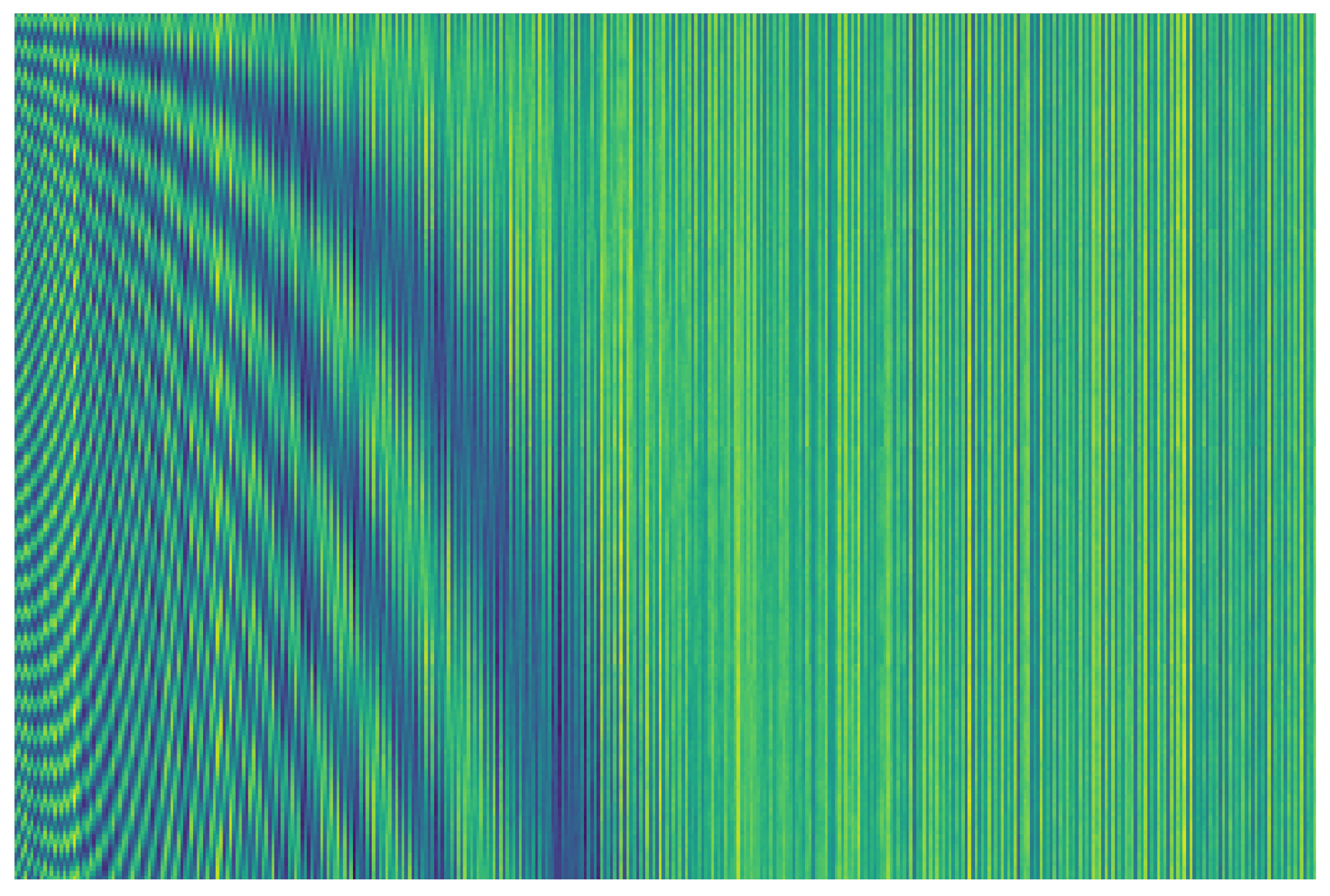
where x is the origin CSI, $pos$ is the position embedding function, and $conv$ is the proposed convolutional neural network. As shown in Figure 3 and Figure 4, we visualize CSI. Compared with the original CSI (in Figure 3), the processed CSI (in Figure 4) has more obvious features between different antennas in the vertical direction, especially between adjacent antenna differences.

3.2. Design of the Dual-Encoder Module

The encoder structure used in the Dual-Encoder module is inspired by the encoder structure in Transformer [37]. The self-attention mechanism enables the encoder structure to pay attention to important information such as channel difference and channel fading through dot product calculation between antennas in CSI. We adopt two encoder structures for parallel computation, and the weights of the two encoders are independent of each other, which allows them to flexibly choose the attention direction. Finally, the outputs of the Dual-Encoder structure are summed to increase the robustness of the model. Additional design details for Dual-Encoder are as follows.

3.2.1. Single Encoder

In actual operation, we make three copies of the entire CSI matrix, and pack them as matrices Q, K, and V, respectively. Here, Q, K, and V are used to obtain the final autocorrelation scores. The autocorrelation calculation formula and multi-focus calculation formula are as follows:

$$Attention(Q,K,V)=softmax(\frac{Q{k}^T}{\sqrt{d_K}})V$$

(4)

$$MultiHead(Q,K,V)=Concat(hea{d}_1,\dots ,hea{d}_n)W^O$$

(5)

where

$$hea{d}_i=Attention(Q{W}_i^Q,K{W}_i^k,V{W}_i^V)$$

(6)

where $W_i^Q\in {\mathbb{R}}^{d_{model}\times d_k}$, $W_i^Q\in {\mathbb{R}}^{d_{model}\times d_k}$, $W_i^Q\in {\mathbb{R}}^{d_{model}\times d_k}$, and $W_i^O\in {\mathbb{R}}^{d_{model}\times d_k}$ are the projections, and $hea{d}_i$ is the dimension of the sub-feature.

3.2.2. Dual-Encoder Structures Are Summed

Considering the feature loss of the CSI matrix in dot product operation, we adopt two encoder structures to encode the CSI matrix separately. Since the two encoder structures are independent of each other, the information they automatically focus on is also different. Complementing the encoding information obtained by the Dual-Encoder structure helps to obtain richer features and improve the robustness of the model. The output formula of the entire Dual-Encoder module is as follows:

$$Encode{r}_{out}=Encode{r}_{one}\left(x\right)+Encode{r}_{two}\left(x\right)$$

(7)

where the x is the output of the Conv-for-Origin module.

3.3. Design of the Conv-for-Sum Module

The function of Conv-for-Sum module is mainly to extract features passed through the Dual-Encoder module, therefore speeding up the convergence of the entire model. The main drawback of MPRI [20] is that the features extracted from the upper part of the model are not concentrated enough. Therefore, in the lower half of the model, two different convolution kernels are used to extract features in parallel on both channels. Finally, the results can be summed up. It seriously affects the convergence speed of the model and increases the depth and training cost of the model. In response to this major flaw, we use serial superposition for the Conv-for-Sum module, which speeds up error propagation, thereby improving the training efficiency of the entire model. Additional design details of Conv-for-Sum are presented in the following subsection.

3.3.1. Two Different Convolution Kernels

To fully extract features from different sub-spaces in CSI, we adopt two convolution layers with different convolution kernels for feature extraction. The convolution layer with a larger $3\times 3$ convolution kernel is responsible for extracting the feature information of the mixed channel, while the convolution layer, with a smaller $1\times 1$ convolution kernel, is responsible for extracting the local antenna features.

3.3.2. Channels of Convolutional Neural Networks

Due to the richness of the CSI feature matrix information, in order to minimize the loss of feature information and to reduce the total number of parameters of the model, we set 256 channels in the convolutional layer. Through experimental comparison, we found that the convergence speed and positioning accuracy of 256 channels are better than fully connected 512- and 128-channel layers in stages.

Moreover, since the extracted feature information is rich, the dimension of the flattened feature is larger. To minimize the risk of overfitting, we use a fully connected three-segment layer.

In summary, we sequentially compute the output of the Conv-for-Sum module using the following equation.

$$Output=BatchNorm\left(ReLU\left(Con{v}_2\left(Con{v}_1\left(X\right)\right)\right)\right)$$

(8)

where X is the output of the Dual-Encoder module and $Con{v}_1$ is the convolutional layer of $3\times 3$ convolution kernel, $Con{v}_2$ is the convolutional layer of the $1\times 1$ convolution kernel, $ReLU$ is the activation function, $BatchNorm$ is the normalization layer, and $Output$ is the output of the Conv-for-Sum module.

4. Experimental Results and Discussion

4.1. Experimental Settings

Experimental Environment: In our experiments, we use a Ubuntu 20.04 server (created by Canonical Ltd, in Isle of Man, UK) with Intel Xeon E5-2650 V2 CPU and a GeForce Tesla P40 GPU for simulations.

Dataset: In terms of datasets, we conduct experiments on two datasets, indoor scenarios, and urban canyon scenarios. The indoor scenario dataset contains 14,448 CSI matrices, of which 11,559 are used for training and 2889 are used for testing, with a split rate of 0.8. The urban canyon scenario dataset contains 11,628 CSI matrices, which are also split into training and test sets with a ratio of 0.8. The datasets used by us can be obtained at https://doi.org/10.21227/jsat-pb50, we have accessed it on 3 May 2020. This two different datasets come from [20]. We describe the extraction process of the dataset as follows. Step 1: Each point’s ray information is obtained with a method that through the aid of the ray-tracing models and completes the electromagnetic analysis of the physical scenario. Step 2: Use a multipath channel filter to package the multipath propagation information into a container with the unit of the user device (UE). Finally, running a system-level simulation of the 5G NR air interface which conforming to the 3GPP standard to obtain the CSI matrices which is the DECC’s input. In deep learning terms, the input features are the CSI matrices, and the output target is the UE’s position in the three-dimensional space.

Training Details: In all training sessions, we use the same parameters for quantitative and qualitative comparisons. During 300 training epochs, the learning rate is set to 2 × 10${}^{-3}$, and the periodic learning rate drop schedule is 50/0.5 (epoch/drop-factor). The optimizer we used is same as that in [38]. During each training process, the testing set is used to evaluate the validation accuracy of the current model. At the same time, the accuracy of the training set is recorded to measure the generalization performance of the model. The training process will be analyzed in the following parts of this section.

4.2. Evaluation Metrics

In the following experiments, we use three metrics widely used to evaluate positioning performance, which are mean error (MeanErr), root mean square error (RMSE), and mean square loss function (MSELoss). The three metrics are defined as follows:

$${\parallel S_i-{\widehat{S}}_i\parallel }_2=\sqrt{{(x_i-{\widehat{x}}_i)}^2+{(y_i-{\widehat{y}}_i)}^2+{(z_i-{\widehat{z}}_i)}^2}$$

(9)

$$MeanError=\frac{1}{N}\sum _{i=1}^{i=N}\left({\parallel S_i-{\widehat{S}}_i\parallel }_2\right)$$

(10)

$$RMSE=\sqrt{\frac{1}{N}\sum _{i=1}^{i=N}{\left(S_i-{\widehat{S}}_i\right)}^2}$$

(11)

$$MSELoss=\frac{1}{N}\sum _{i=1}^{i=N}\left[{(x_i-{\widehat{x}}_i)}^2+{(y_i-{\widehat{y}}_i)}^2+{(z_i-{\widehat{z}}_i)}^2\right]$$

(12)

where ${\widehat{x}}_i$, ${\widehat{y}}_i$, and ${\widehat{z}}_i$ denote the estimated three-dimensional coordinates of the i-th data, and $x_i$, $y_i$, and $z_i$ represent the actual 3D coordinates of the i-th data, respectively, so ${\widehat{S}}_i$ and $S_i$ are the estimated position of the i-th data and the actual position of the i-th data, respectively. Additionally, ${\parallel ·\parallel }_2$ denotes the Euclidean distance.

4.3. Generalization and Convergence Analysis

For deep learning network models, generalization refers to the ability of the model to apply to new data after training and to make accurate predictions, while convergence refers to the stability and reliability of the model, and so testing the convergence and generalization of deep learning models is significant.

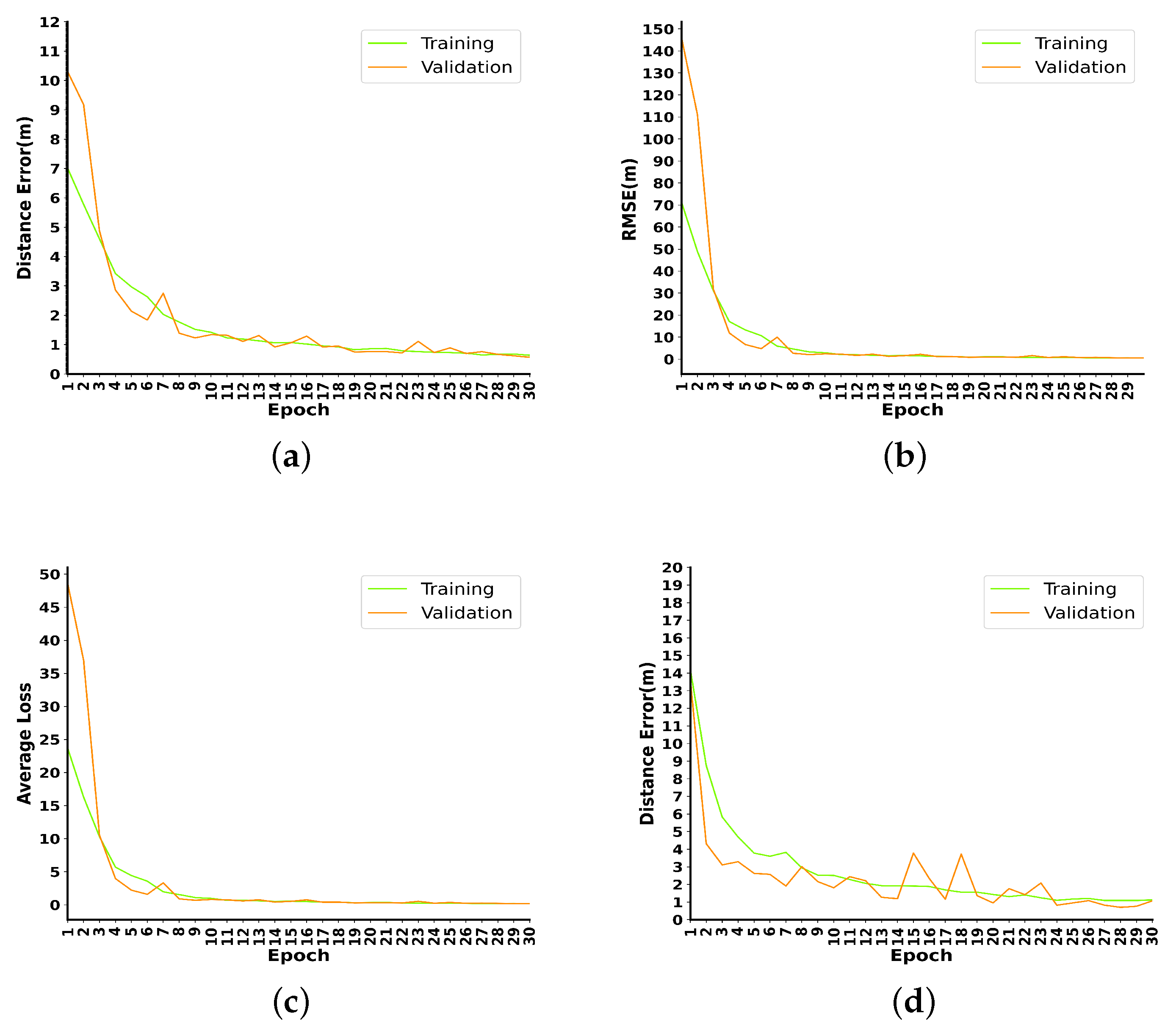
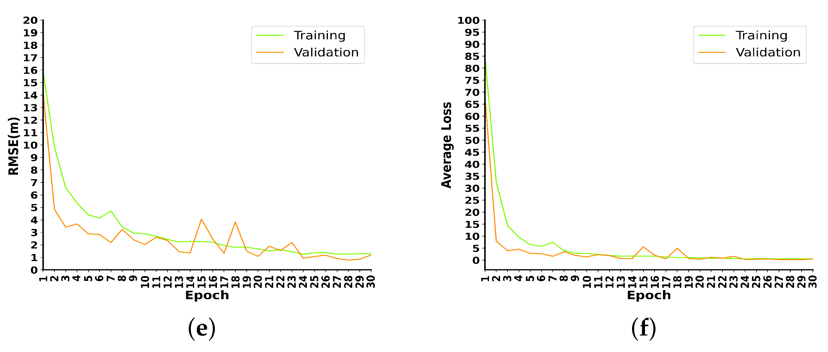
The MeanError, RMSE, and MSELoss tests for the urban canyon and indoor datasets are shown in Figure 5. In the first 30 training sessions, the RMSE in the urban canyon scene drops from 14.2 to 1.12; MeanError drops from 13.6 to 1.02; the MSELoss drops from 68.2 to 0.42. In the indoor scene, RMSE drops from 71.3 to 0.55; MeanError drops from 7.01 to 0.64; and MSELoss drops from 23.7 to 0.18. It can be seen from the figure that the curves of the training set and the validation set are always close in three indicators; especially in the test of the urban canyon dataset, the effect of the test set is slightly better than that of the training set, and there is no overfitting phenomenon.

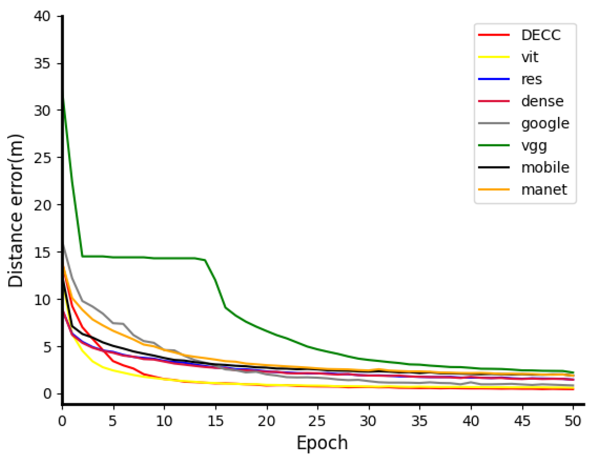
We introduce other classic outstanding DNNs for comparison, namely Vit_b_16 [39], ResNet18 [18], Vgg [31], Densenet [40], Mnasnet [41], GoogLeNet [19], and Mobilenet_v3 [21]. As shown in Figure 6, DECC is significantly faster than that of Vgg, ResNet18, and GoogLeNet, in terms of convergence speed. In the first 25 rounds, the convergence effect of DECC is close to vit_b_16, and superior to vit_b_16 in the last 25 rounds.

It can be seen from the above tests that the generalization performance and convergence effect of DECC can be proven on both datasets.

4.4. Positioning Accuracy

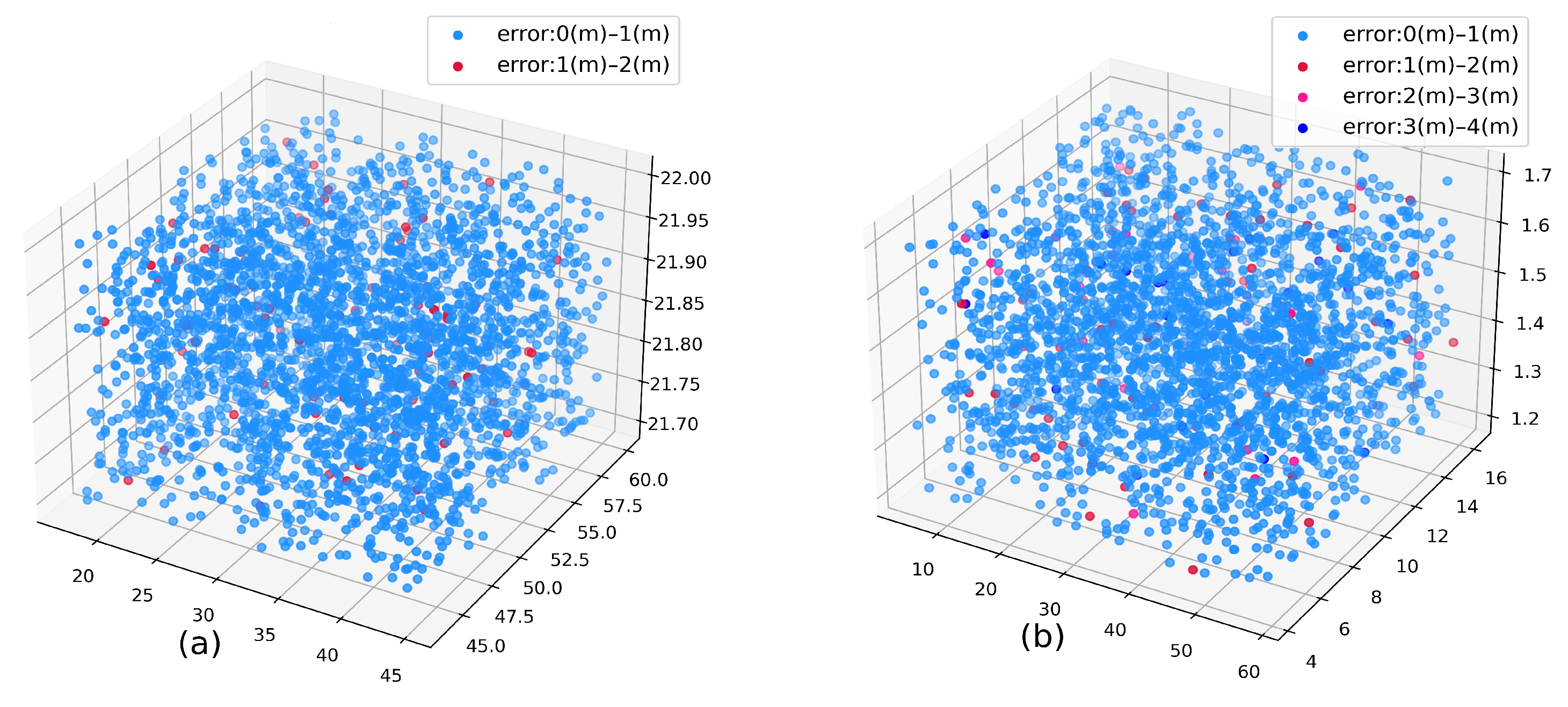
In this section, we set up two experiments to verify the stability and performance differences of DECC. The positioning performance of urban canyons and indoor scenes is shown in Figure 7a,b, and the ablation experiment is shown in Figure 8a,b.

Numbered lists can be added as follows:

(1)

Exp. 1: Urban Canyon and Indoor Scenario—In the urban canyon scene, the average error is 0.18 m, 91% of the point errors are less than 0.5 m, 98% of the points errors are less than 1 m, and only a few points have an error of more than 1 m. In the indoor scene, the average error is 0.26 m, 92% of the points are smaller than 0.5 m, 96% of the points are less than 1 m, and only a small part of the points are more than 1 m.

(2)

Exp. 2: Ablation Experiment for the DECC—In order to verify the performance of DECC, we carry out the burning experiment in an indoor scene. First, we take the full version of DECC as the control group, and DECC with only the Dual-Encoder structure as the control group 1, and with only the Conv-for-Sum module as control group 2.

As shown in Figure 8b, we can observe that the control group achieves positioning accuracy with an average error of 0.26 m, while the accuracies of control groups 1 and 2 are 17.2 m and 18.1 m, respectively. The performance has increased by 16.72 m and 17.62 m, respectively.

Moreover, in terms of standard deviation, the standard deviation of the control group is 0.28 m, which is significantly higher than those of control groups 1 and 2 (5.2 m and 6.0 m). The results show that due to the superiority of the model, the full DECC has great advantages in positioning accuracy and stability.

In summary, our proposed method achieves good results for both complex indoor environments and open urban canyon scenarios.

4.5. Frequency Robustness

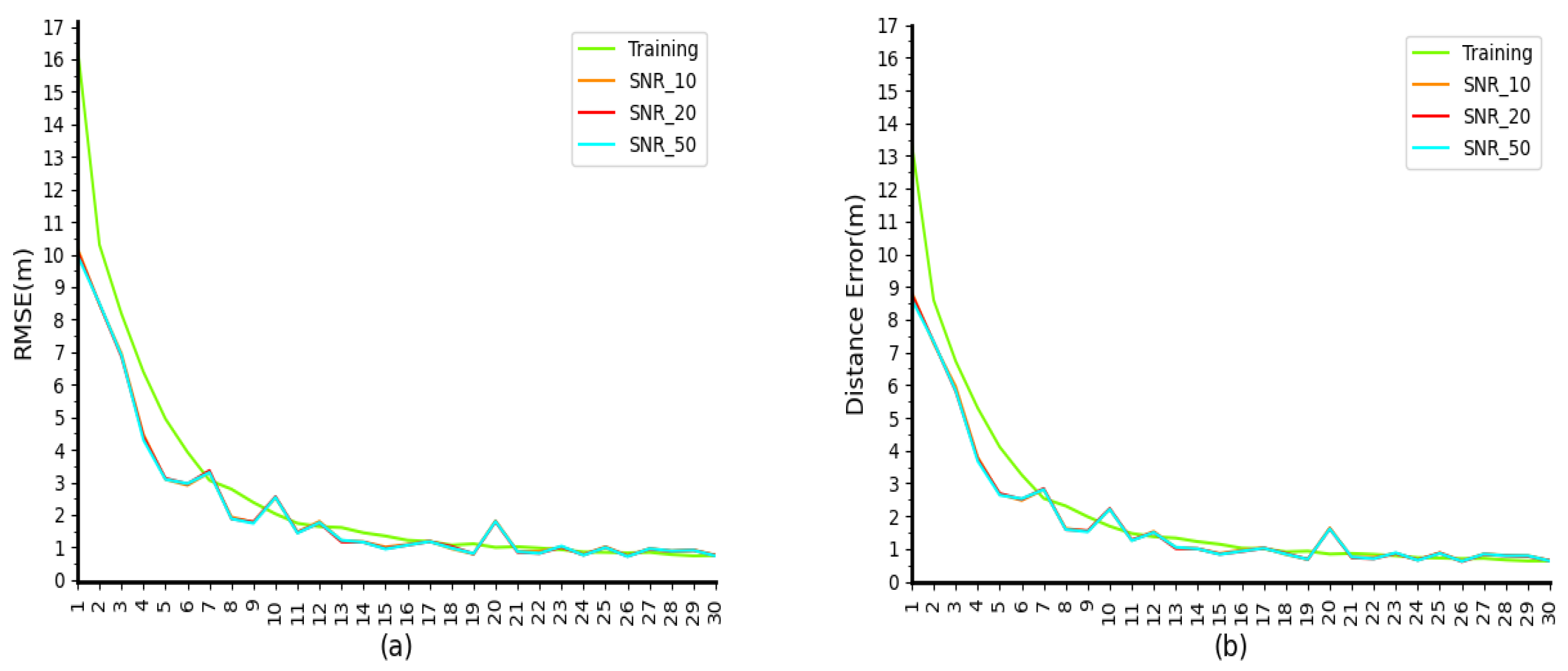
In the experiments, to check the robustness of proposed DECC at SNR, we set up a control group and three experimental groups to analyze the robustness of DECC to signals with different SNRs. The control group is shown in Section 4.2, i.e., 80% of the overall mixed SNR dataset is used for training and 20% is used for testing. Experimental group 1 was trained with the same mixed SNR dataset and tested with only the same number of SNR10 datasets as the control group. The training set of experimental group 2 is the same as above, and the test set uses the same number of SNR20 datasets. The training set of experimental group 3 is the same as above, and the test set uses the same number of SNR50 datasets. As can be seen from Figure 9 and Figure 10, when only the three datasets—SNR10, SNR20, and SNR50—are used to test the model, the results—0.27, 0.26, and 0.26, respectively—are similar to those of the control group, indicating that our model can achieve relatively stable results under different signal-to-noise ratios.

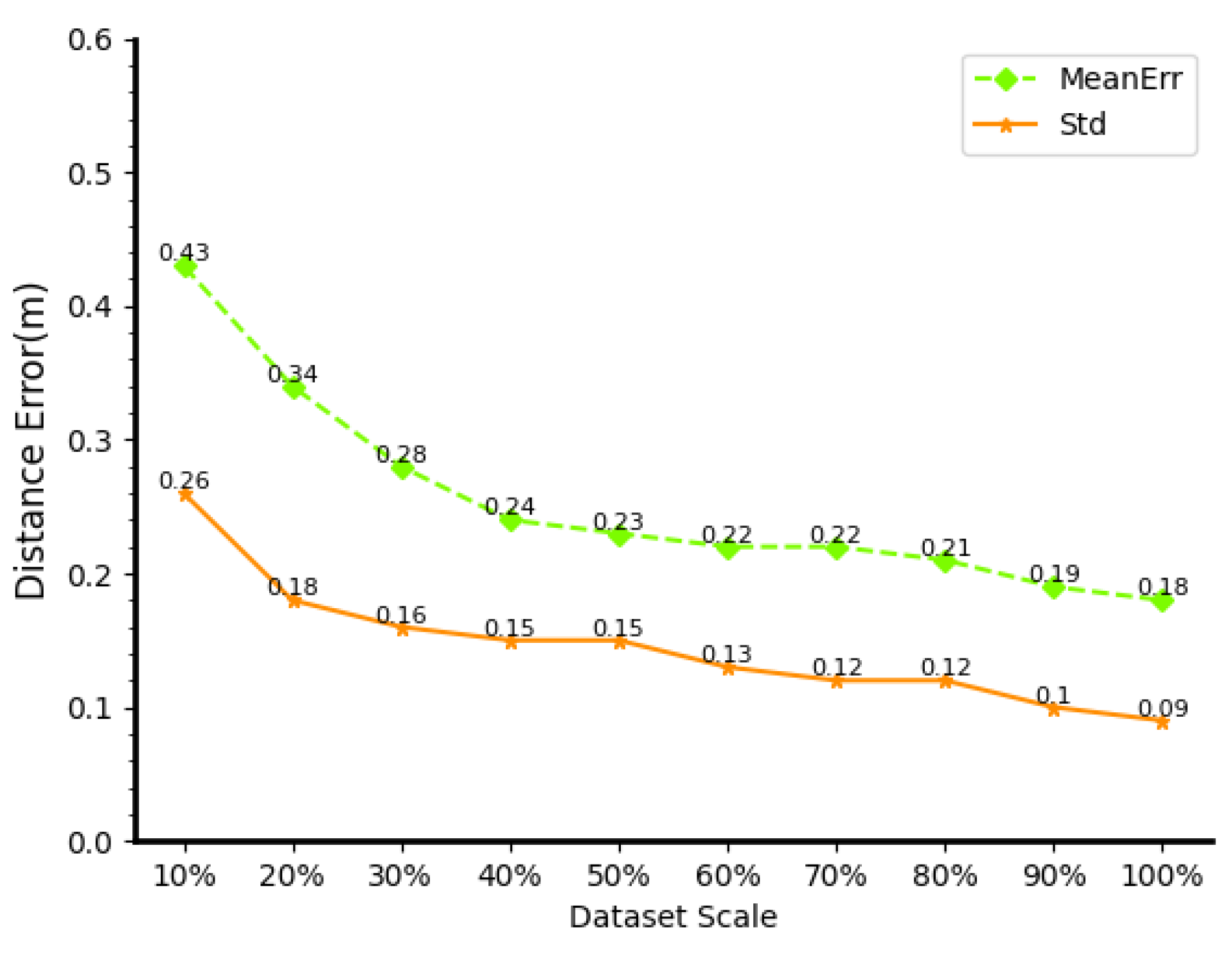
4.6. Robustness-to-Dataset Scale

In a real-world setting, this section analyzes the impact of dataset size on the robustness of DECC. Generating an easy-to-use, high-quality, and understandable dataset is extremely difficult, and will incur huge costs in terms of time, labor, and finances as the amount of data increases. At the same time, massive data will bring fatal problems to deep learning models, due to the cost of operation, maintenance, and training. Therefore, we verify the accuracy comparison of DECC in datasets of different sizes to verify the robustness of DECC to the number of datasets. DECC is trained on 10%, 20%, 30%, 40%, 50%, 60%, 70%, 80%, and 90% of the original dataset, used as the experimental group, and DECCs trained on the full original dataset (14,448 CSI), which served as the control group for comparison experiments, as shown in Figure 11.

From experimental group 1 to experimental group 9, the mean error increases by 138% and 5%, respectively. As the dataset size increases, the training results become closer and closer to the control group. The mean error for experimental group 9 was 0.19, which was only 0.01 away from the control group. Experimental group 1 only used less than 1500 images (randomly sampled from SNR10, 20, and 50, trained 200 times, but the average error was still 0.43 m, reaching sub-meter accuracy. This shows that DECC can still achieve ideal results, even when the amount of data is small and the number of training times is low, and the positioning accuracy can be further improved with the expansion of the dataset, which shows that DECC has high practical application value.

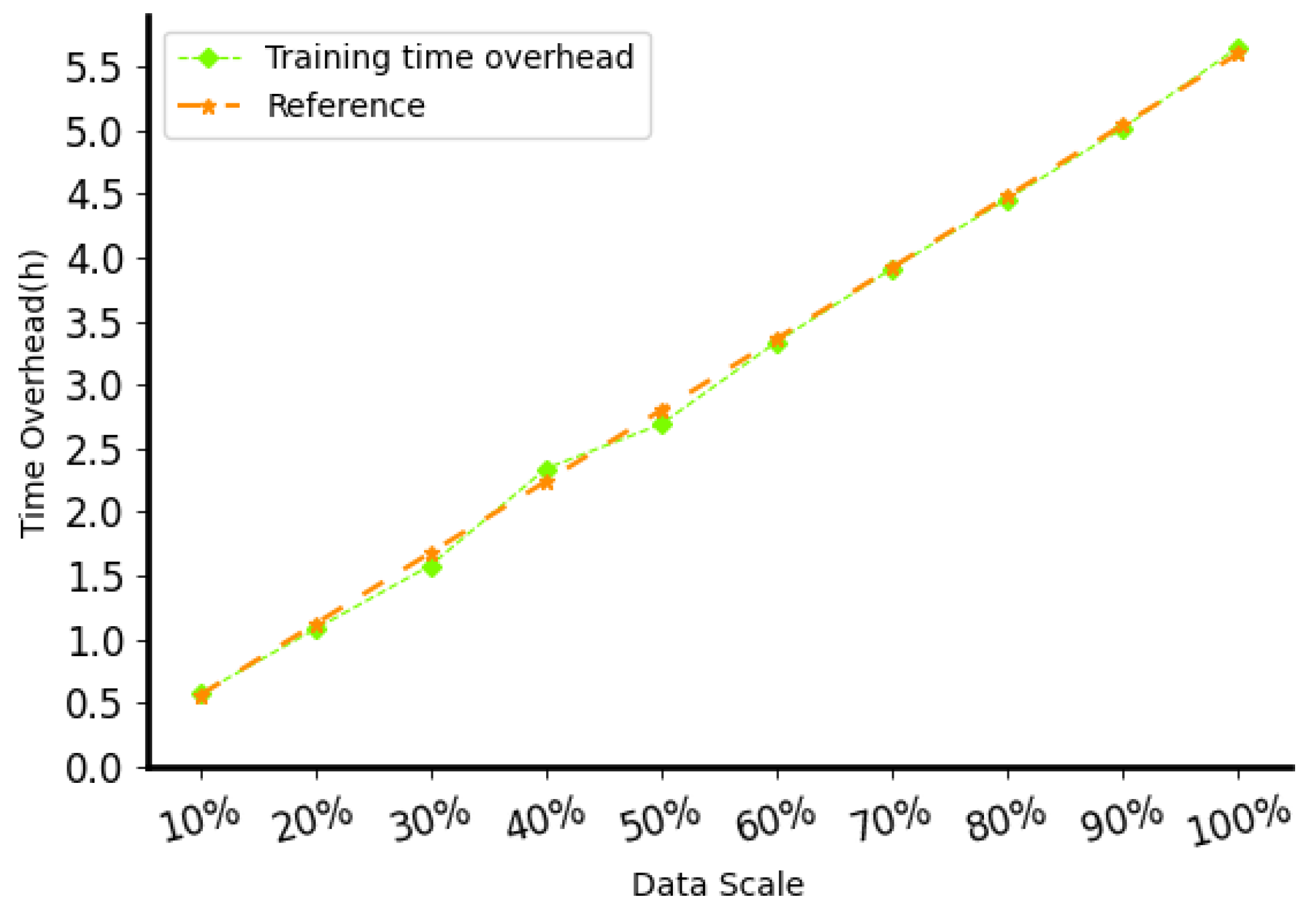
4.7. Time Overheads

In this section, we study the training time and the localization prediction time (letter rate). Figure 12 shows the training time cost of DECC on datasets of different scales described in the previous section. We set the number of sessions per case under the dataset partition to 200. We found that the change in time consumption is basically linear, with 1440 data points training in approximately 34 min, 4320 data points in 1 h and 44 min, and 11,568 data points in 4 h and 36 min. We also tested how fast DECC can calculate 3D position (real-time localization). We give DECC 1000 localization tasks (batch size set to 16) to calculate “time per thousand localizations” (TPT). When the test was repeated 200 times, the average TPT was 2.78 s, indicating that each task took less than 0.002 s. These results show that the DECC method can achieve a positioning refresh rate of more than 500 Hz, which is sufficient to meet the real-time positioning requirements of objects moving at a medium speed.

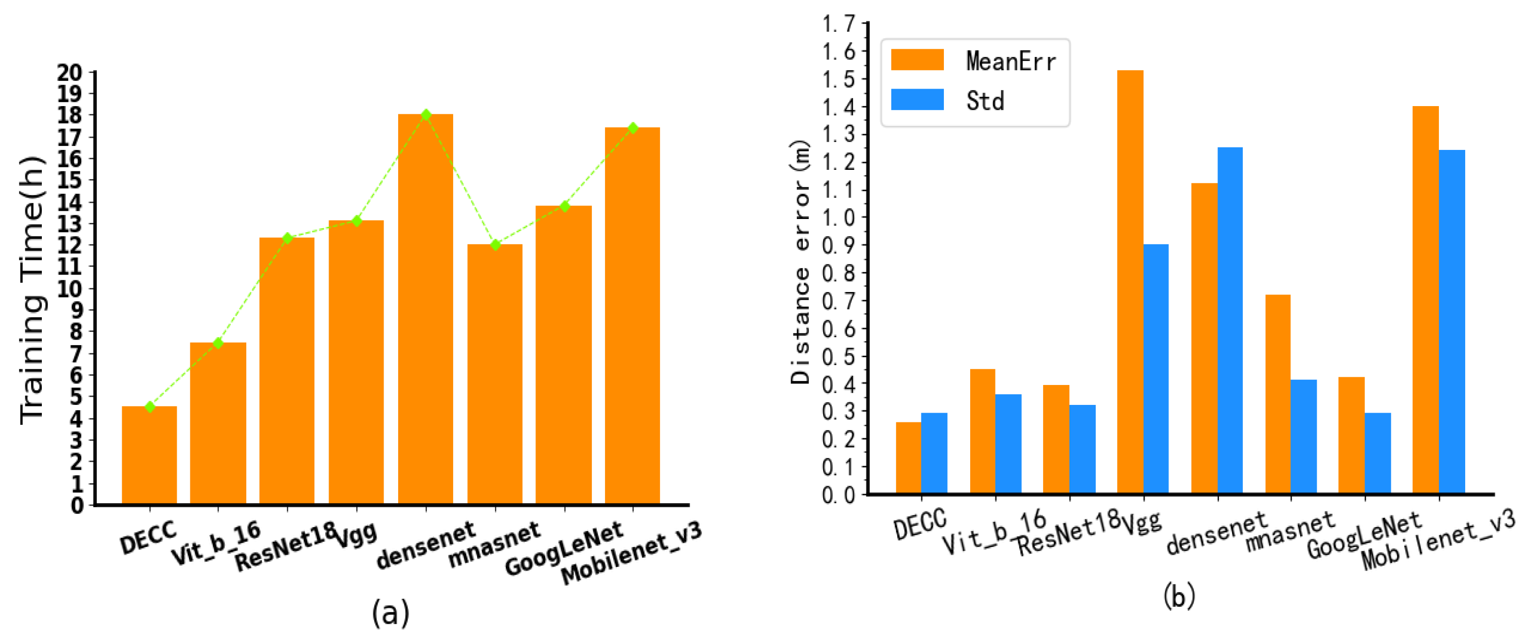
4.8. Comparison with Classic DL Methods

In this section, we make a comparative analysis of several classical deep learning networks with the proposed DECC. The DECCs put forward by the test group are our network and the control group, including seven other DL models, i.e., Vit_b_16 [39], ResNet18 [18], Vgg [31], Densenet [40], Mnasnet [41], GoogLeNet [19], and Mobilenet_v3 [21]. The DECC we used for comparative analysis has 3 layers of Dual-Encoder and 15 layers of Conv-for-Sum. For the other networks, to obtain the best positioning precision, we stopped when it converges to the best result of smooth.

In terms of time overheads, as shown in Figure 13a, the DECC has 4.5 h of training cost, and Vit_b_16 [39], ResNet18 [18], Vgg [31], Densenet [40], Mnasnet [41], and GoogLeNet [19] are 40%, 64%, 66%, 75%, 62%, 68%, and 75% less than Mobilenet_v3 [21] %, respectively.

As shown in Figure 13b, the network positioning accuracy of DECC is 0.26 m, and the mean square error is less than 0.30, compared with Vit_b_16 [39], ResNet18 [18], Vgg [31], Densenet [40], Mnasnet [41], GoogLeNet [19], and Mobilenet_v3 [21], which increased by 73%, 50%, 488%, 330%, 176%, 62%, and 438%, respectively. This shows that, while it improves the positioning accuracy, it also improves the training efficiency, and so our proposed DECC has high practical application value.

5. Conclusions

This paper studies the application of deep learning models in high-precision indoor positioning, and proposes a deep learning model, DECC, for high-precision indoor positioning. Specifically, we design two different convolution modules to extract information from raw CSI features and encoded CSI features, respectively. In addition, in the middle part of the model, we use a self-attention-based dual encoder to explore the channel differences and correlations between different antennas. Experiments on real localization data demonstrate the high accuracy and efficiency of DECC localization in different scenarios.

We provide a feasible scheme to apply our proposed DECC to the real scenario. First, pre-train our DECC on the dataset to obtain the offline model which stores the updated parameters and converts the offline model file format for the positioning system to the calling format. Secondly, run a system-level simulation of the 5G NR air interface which conforms to the 3GPP standard to estimate the CSI matrices for the target to be estimated. Thirdly, put the CSI matrices into the pre-train model or the positioning system with the pre-train model to obtain the estimated position. We used a laptop computer to evaluate feasibility from a practical point of view. Specifically, we input 2320 obtained CSI matrices with every 16 into the pre-train model to simulate high-concurrence and high-request scenarios. The results showed that even with the lower performance mobile device with the RTX 3060 GPU and i7-11800H CPU, the total process only took 4.37 s—less than 0.0019 s were taken to locate a unit. It is also worth noting that 2320 obtained CSI matrices came from a room of less than 700 square meters in size. In the real world, such intensive requests are unlikely to occur. So, our feasibility evaluation satisfied two extreme cases: (1) unusually high concurrency requests; (2) lack of high-performance equipment.