Hierarchical Superpixel Segmentation for PolSAR Images Based on the Boruvka Algorithm

Abstract

Superpixel segmentation for polarimetric synthetic aperture radar (PolSAR) images plays a key role in remote-sensing tasks, such as ship detection and land-cover classification. However, the existing methods cannot directly generate multi-scale superpixels in a hierarchical style and they will take a long time when multi-scale segmentation is executed separately. In this article, we propose an effective and accurate hierarchical superpixel segmentation method, by introducing a minimum spanning tree (MST) algorithm called the Boruvka algorithm. To accurately measure the difference between neighboring pixels, we obtain the scattering mechanism information derived from the model-based refined 5-component decomposition (RFCD) and construct a comprehensive dissimilarity measure. In addition, the edge strength map and homogeneity measurement are considered to make use of the structural and spatial distribution information in the PolSAR image. On this basis, we can generate superpixels using the distance metric along with the MST framework. The proposed method can maintain good segmentation accuracy at multiple scales, and it generates superpixels in real time. According to the experimental results on the ESAR and AIRSAR datasets, our method is faster than the current state-of-the-art algorithms and preserves somewhat more image details in different segmentation scales.

1. Introduction

Polarimetric synthetic aperture radar (PolSAR) is widely applied for various remote sensing applications, such as land use land cover (LULC) classification [1,2,3,4] and ship detection [5], due to its great advantages in providing informative images under all weather conditions, day or night. In recent years, object-based classification and detection for SAR and PolSAR images is becoming more and more popular, since it can alleviate the inherent speckle noise and preserve the structure information of the objects. The accurate segmented superpixels can be used as basic elements of large-sized images, which can greatly simplify subsequent processing, such as object-based classification [6] and region-based ship detection [7,8]. In addition, compared with the pixel-level processing algorithms, superpixel-based methods have improved timeliness. Therefore, superpixel segmentation plays a fundamental role in this field, and it determines the performance of subsequent interpretation tasks to a large extent.

There are many representative state-of-the-art superpixel segmentation methods originally designed for optical images, such as simple linear iterative clustering (SLIC) [9], normalized cuts (N-cuts) [10], linear spectral clustering (LSC) [11], and mean shift [12]. Numerous superpixel segmentation methods are based on feature clustering. The SLIC method is a local clustering method constrained by the CIELAB color space distance and coordinate distance. The superpixel results of SLIC are very compact and have similar and regular sizes. It also has an ideal time efficiency. To make the SLIC method applicable to PolSAR images, Qin et al. [13] used the revised Wishart distance, Song et al. [14] used the symmetric revised Wishart distance, and Feng et al. [15] used the Bartlett distance to replace the color distance by taking into account the statistical characteristics of PolSAR data. Other researchers [16,17] modified the original SLIC by applying the elements derived from Pauli and Cloude decomposition. Zhang et al. [18] built a scattering mechanism feature vector and calculated its Euclidean distance instead of Wishart distance in [13]. It can reduce the time cost due to reduced matrix operations. Xiang et al. [19] proposed an adaptive polarimetric SLIC (Pol-ASLIC) superpixel generation method, utilizing a homogeneity measurement (HoM) as a tradeoff factor to control the segments’ shape and compactness. Lin et al. [20] proposed a K-means-based segmentation method with a new distance function and superpixel seed updating strategy for PolSAR images. Quan et al. [21] constructed a feature vector through results from refined five-component decomposition (RFCD) and other scattering mechanism features, and used the linear feature local clustering (LFLC) method to generate superpixels. However, these clustering-based methods only take local properties into consideration and cannot obtain size-adaptive superpixels from a global perspective. Xu et al. [22] proposed a polarimetric semivariogram-based spatial scale selection method for PolSAR image segmentation with a mean shift algorithm. Lang et al. [23] further developed the generalized mean shift algorithm for PolSAR superpixel generation and defined a new merging predicate defined in the joint spatial-range domain. The mean shift method iteratively refines the clusters to form superpixels. However, it ignores the compactness constraints, which makes the shape of the superpixels highly irregular.

The graph-based method considers pixels as nodes and treats the image to be segmented as a weighted undirected graph. The segmentation is achieved by removing the edges and those generated sub-graphs corresponding to the superpixel results of polarimetric SAR images. Liu et al. [24] applied the normalized cuts method to generate superpixels for PolSAR based on edge maps derived from the revised Wishart distance. Xu et al. [25] proposed an object-based N-cuts method on the basis of results of the SLIC method for high-resolution PolSAR images. The normalized cuts algorithm can generate regular and compact image fragments, and due to its global strategy, the global image structure is preserved. However, it requires very high computational complexity as there are plenty of eigen-based calculations, which makes it unsuitable for large size segmentation. Wang et al. [26] incorporated spherically invariant random vector (SIRV) distance into the entropy rate algorithm framework to generate superpixels for PolSAR images. It can adaptively select a suitable distance metric according to the homogeneity, but the computation time of two types of distance is too long. Lin et al. [27] merged small blocks based on the minimum spanning tree (MST) structure to achieve segmentation for high-resolution remote sensing images. Although it is fast, it sacrifices segmentation accuracy due to the use of blocks and the results are not superpixels.

The hierarchical or multiscale segmentation can facilitate PolSAR image analysis tasks such as semantic segmentation and saliency detection [28]. The hierarchical structure of a PolSAR image should allow large-sized superpixels to be composed of smaller ones, which can extract much more details at a small scale while preserving global structure. To achieve the multiscale segmentation, those aforementioned methods cannot obtain the results directly and must repeat the whole segmenting procedure or add a merging operation, which leads to low efficiency [29].

Based on the framework of the Boruvka method and the method of calculating the edge strength inspired by [30,31], we proposed a novel hierarchical segmentation method for PolSAR images, which can generate different scales of superpixels in real time. The distance measure between the pixels is mainly described by the polarimetric scattering feature that is decomposed by RFCD [32]. Additionally, the edge strength information based on the statistical Wishart distance and homogeneity measurement are also considered to help improve segmentation accuracy. Our method creates one MST structure of the PolSAR image and cuts the edges with largest weight to undertake superpixel segmentation.

The main content of this article consists of the following parts. Section 2 provides the explanation of the methodology. It firstly presents the basic theory of PolSAR data with its distribution and introduces the method of model-based 5-component decomposition, and then introduces the construction of a distance measure. The segmentation method based on the Boruvka algorithm is proposed finally. In Section 3, the performance of our algorithm is demonstrated using the PolSAR dataset from the ESAR system and AIRSAR system. Section 4 presents the discussion and Section 5 concludes this paper.

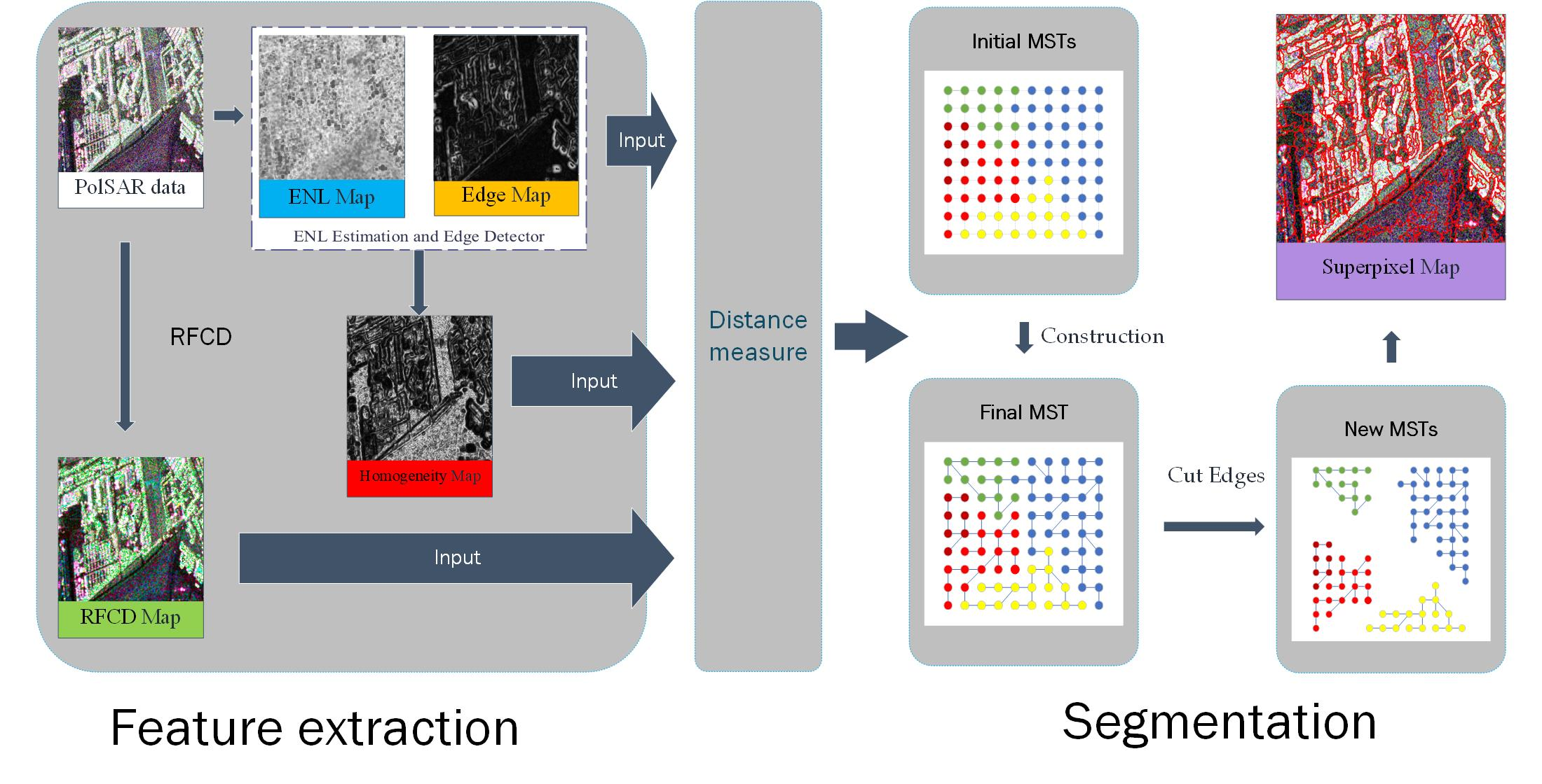
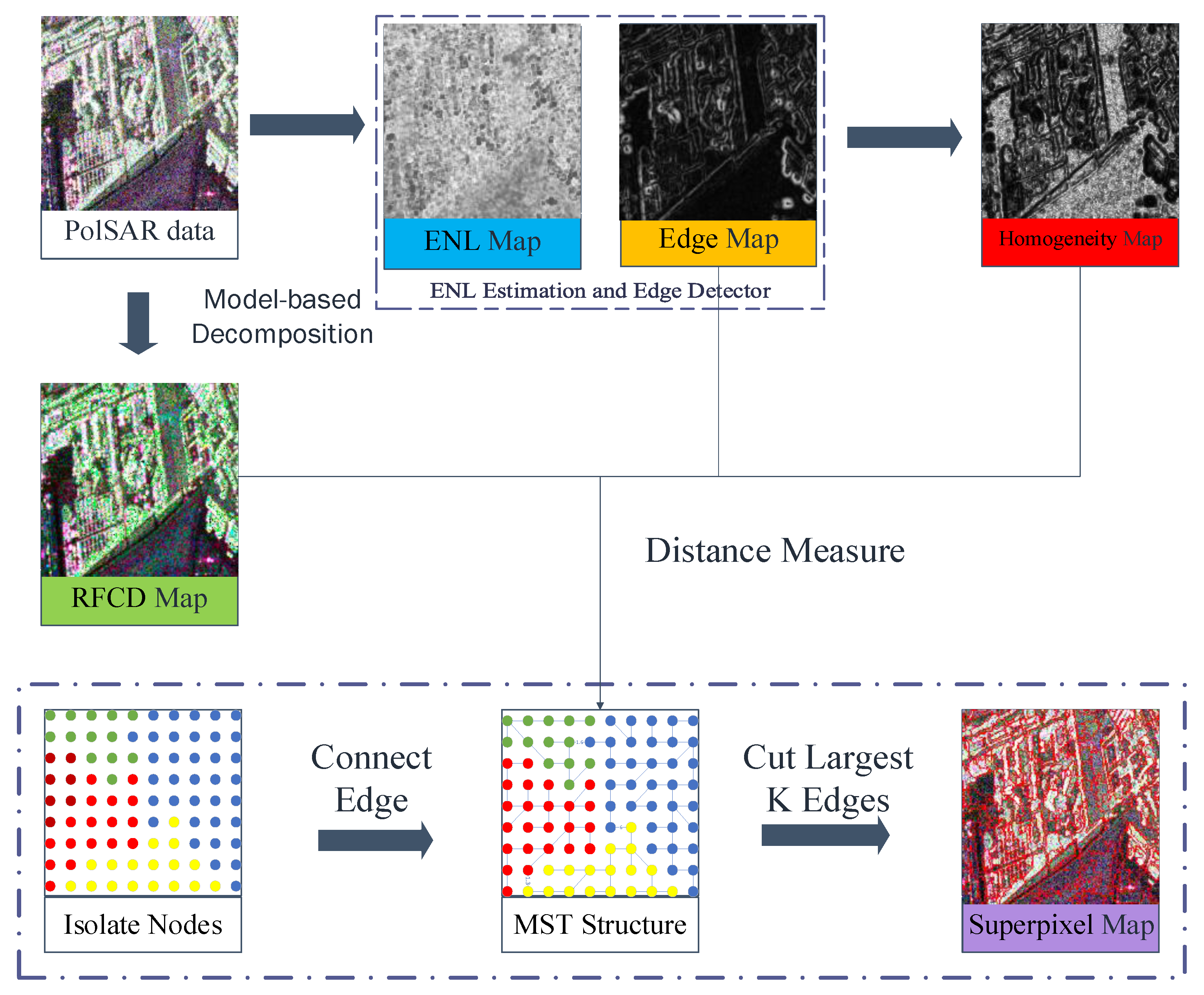
2. Methodology

2.1. PolSAR Data

2.1.1. Wishart Distribution and Wishart Distance

The fully polarimetric SAR uses a 4×4 complex scattering matrix to characterize the scattering phenomenon of the target to the incident wave. For a reciprocal target illuminated by a monostatic SAR, the polarimetric scattering information can be represented in the form of a scattering vector k using the Pauli basis [26]

$$k=\frac{1}{\sqrt{2}}{[S_{HH}+S_{VV},S_{HH}-S_{VV},2S_{HV}]}^T$$

(1)

where $S_{HH}$, $S_{HV}$, and $S_{VV}$ are the complex scattering coefficients, representing the HH, HV, and VV polarizations, while $S_{VH}=S_{HV}$. The superscript T means the matrix transposition. In homogeneous areas, PolSAR data can be modeled with a multivariate zero-mean circular Gaussian distribution. For multi-look PolSAR data, the polarimetric information can be presented in the form of a coherence matrix [33]

$$T=\frac{1}{L}{\displaystyle \sum _{i=1}^L{k}_i{k}_i{}^{*T}}$$

(2)

where the superscript * means the complex conjugate and L is the number of looks. Let $Z=LT$, and the matrix $Z$ follows the complex Wishart distribution. Let $\mathsf{\sum }=E\left\{k{k}^{*T}\right\}$. The probability density function (PDF) [34] of T is

$$p(\mathit{T},\sum )=\frac{L^{qL}{\left|\mathit{T}\right|}^{L-q}\exp (-L\mathrm{Tr}({\sum }^{-1}\mathit{T}))}{K(L,q){\left|\sum \right|}^L}$$

(3)

$$K(L,q)={\pi }^{q(q-1)/2}{\displaystyle \mathsf{\prod }_{i=1}^q\mathsf{\Gamma }(L-i+1)}$$

(4)

where $\sum =E\left\{k{k}^{*T}\right\}$ and variable $q$ is the dimension of $k$ (q = 3 in monostatic SAR situation). Tr(·) and |·| denote the trace and determinant of a matrix and Γ(·) is the Gamma function.

The test statistic in [35] is used to deduce the dissimilarity between two regions, which is called the revised Wishart distance, and its formula is provided as

$$d_{RW}(R_i,R_j)=\ln (\frac{\left|{{\displaystyle \widehat{\sum }}}_j\right|}{\left|{{\displaystyle \widehat{\sum }}}_i\right|})+Tr({{\displaystyle \widehat{\sum }}}_j{}^{-1}{{\displaystyle \widehat{\sum }}}_i)-q.$$

(5)

The ${{\displaystyle \widehat{\sum }}}_i$ and ${{\displaystyle \widehat{\sum }}}_j$ are the center coherence matrices of regions $R_i$ and $R_j$. If i = j, $d_{RW}(R_i,R_j)$ equals zero, the minimum value; else, the value of $d_{RW}(R_i,R_j)$ is larger than zero.

2.1.2. Refined Five-Component Decomposition

In order to better distinguish pixels of different categories in order to facilitate fine segmentation, we adopted the refined five-component-model-based decomposition to construct a feature vector. The polarimetric decomposition methods can describe the physical scattering mechanism models with sub-matrices of the measured coherency matrix. Quan et al. [32] decomposed the measured coherency matrix into the following five submatrices,

$$\begin{array}{c}〈[T]〉=\left[\begin{array}{ccc}{T}_{11}& T_{12}& T_{13}\\ T_{21}& T_{22}& T_{23}\\ T_{31}& T_{32}& T_{33}\end{array}\right]\\ \hspace{1em}\hspace{1em}\hspace{1em}\hspace{1em}\hspace{1em}\hspace{1em}\hspace{1em}\hspace{1em}\hspace{1em}\hspace{1em}\hspace{1em}\hspace{1em}\hspace{1em}=f_S{[T]}_S+f_D{[T]}_D+f_V{[T]}_V+f_H{[T]}_H+f_O{[T]}_O\end{array}$$

(6)

where $f_i(i=S,D,V,H,O)$ expresses the scattering coefficients and ${[T]}_i(i=S,D,V,H)$ is the scattering model in Yamaguchi 4-component decomposition [36] (surface, double-bounce, volume, and helix), and ${\left[T\right]}_O$ is a scattering model of obliquely oriented buildings (OOBs) based on the fact that the cross-pol components are much larger than the co-pol ones. The formula (6) can be expanded explicitly into

$$\begin{array}{c}\left[\begin{array}{ccc}{T}_{11}& T_{12}& T_{13}\\ T_{21}& T_{22}& T_{23}\\ T_{31}& T_{32}& T_{33}\end{array}\right]=f_S\left[\begin{array}{ccc}1& {\beta }^{*}& 0\\ \beta & |\beta {|}^2& 0\\ 0& 0& 0\end{array}\right]+f_D\left[\begin{array}{ccc}|\alpha {|}^2& \alpha & 0\\ {\alpha }^{*}& 1& 0\\ 0& 0& 0\end{array}\right]+\frac{f_V}{4}\left[\begin{array}{ccc}2& 0& 0\\ 0& 1& 0\\ 0& 0& 0\end{array}\right]\\ +\frac{f_H}{2}\left[\begin{array}{ccc}0& 0& 0\\ 0& 1& \pm j\\ 0& \mp j& 1\end{array}\right]+f_O\left[\begin{array}{ccc}0& 0& 0\\ 0& O_{22}& 0\\ 0& 0& O_{33}\end{array}\right].\end{array}$$

(7)

$\alpha$ and $\beta$ are the model parameters of double-bounce scattering and surface scattering. The $O_{22}$ and $O_{33}$ have the following expressions [32],

$$O_{22}=\frac{C_{OOB}}{C_{OOB}+\frac{C_{OOB}}{M-C_{OOB}+\xi }},O_{33}=\frac{\frac{C_{OOB}}{M-C_{OOB}+\xi }}{C_{OOB}+\frac{C_{OOB}}{M-C_{OOB}+\xi }}$$

(8)

where $C_{OOB}$ denotes the scattering characteristics of OOBS [37]. The factor $M$ is the maximum of $C_{OOB}$ and $\xi$ is an infinitely small positive number. Additionally, a set of equations need to be solved, i.e.,

$$\begin{array}{l}{f}_S+f_D|\alpha {|}^2+\frac{f_V}{2}=T_{11}\\ f_S|\beta {|}^2+f_D+\frac{f_V}{4}+\frac{f_H}{2}+f_O{O}_{22}=T_{22}\\ \frac{f_V}{4}+\frac{f_H}{2}+f_O{O}_{33}=T_{33}\\ f_S{\beta }^{*}+f_D\alpha =T_{12}\\ \frac{f_H}{2}=|\mathrm{Im}(T_{23})|.\end{array}$$

(9)

By reducing the unknowns step by step, the final scattering contribution results $P_S$, $P_D$,$P_V$, $P_H$, and $P_O$ are acquired as

$$\begin{array}{l}{P}_S=f_S(1+|\beta {|}^2),P_D=f_D(1+|\alpha {|}^2)\\ P_H=f_H,P_O=f_O,P_V=f_V\end{array}$$

(10)

The experimental results demonstrated the favorable performance in characterizing the scattering difference among buildings with orientations. On this basis, we can measure the dissimilarity of the PolSAR pixels.

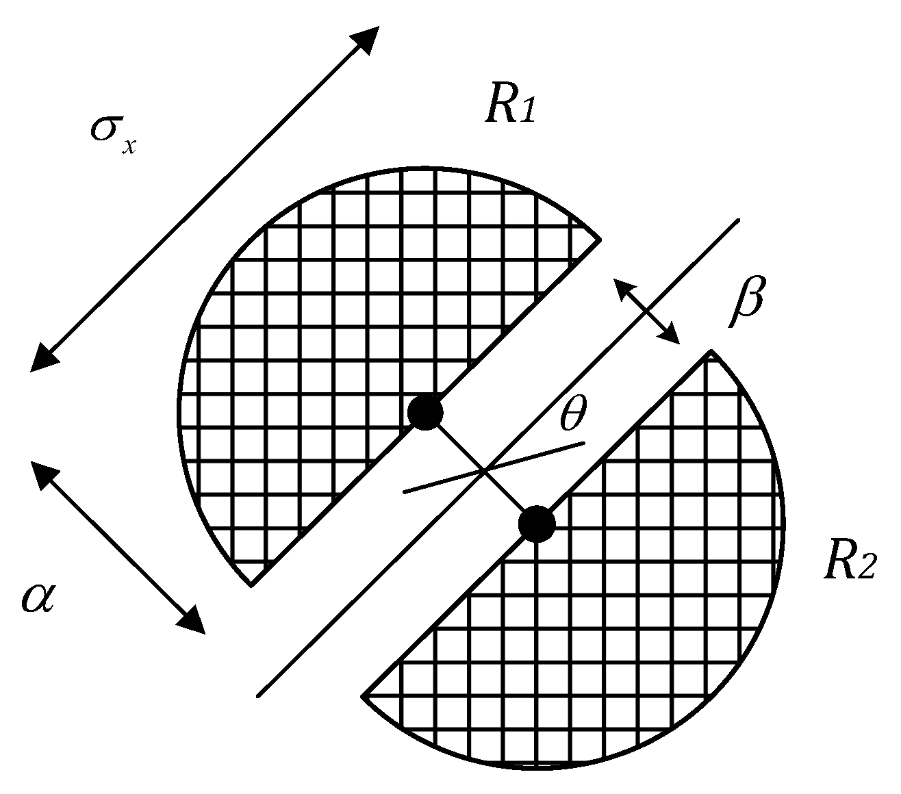
2.2. Distance Measure Construction

The PolSAR data in different areas reflect various scattering properties, and the distance to measure the corresponding difference in PolSAR imagery is a critical factor that determines the accuracy of superpixel segmentation. The RFCD feature has shown to have great physical scattering interpretation in superpixel segmentation [21]. Therefore, we choose the RFCD feature as the basis for the distance metric. In addition, the edge and homogeneity information are added to help improve the segmentation performance. We can form a feature vector of each pixel with the normalized scattering power,

$$v_s=\left[\begin{array}{ccccc}{P}_S& P_D& P_V& P_H& P_O\end{array}\right].$$

(11)

Thus, the distance [38] of the 5-D feature vector is considered to measure the dissimilarity between neighboring pixels i and j from the perspective of the backscattering mechanism

$$D_S=\sqrt{2{\displaystyle \sum _{k}M\ln \frac{|{\overline{P}}_{ik}+{\overline{P}}_{jk}|}{2\sqrt{{\overline{P}}_{ik}{\overline{P}}_{jk}}}}},k=S,D,V,H,O.$$

(12)

The data is averaged using a M = 3 × 3 size boxcar filter to alleviate the effect of speckle noise.

The edge information that describes the structural details in the image is beneficial for improving the segmentation accuracy. Therefore, it is utilized in the proposed method. The edge strength map (hereafter denoted as EDGE) is extracted based on the edge detector in [39,40]. In this paper, the Gauss–Gamma-shaped filter replaces the rectangle-shaped filter to estimate the coherence matrix within a region. As shown in Figure 1, the Gauss–Gamma-shaped window provides larger weights of the pixels near the center pixel than those far from the center pixel, therefore, it can estimate the coherence matrix with higher accuracy than the rectangle filter. In Figure 1, the two horizontal Gauss–Gamma-shaped 2-D window functions of $R_1$ and $R_2$ in position $(x,y)$ are

$$\begin{array}{l}{W}_U(x,y)\frac{|y{|}^{\alpha -1}}{\sqrt{2\pi }{\sigma }_x\mathsf{\Gamma }(\alpha ){\beta }^{\alpha }}\exp (-(\frac{x^2}{2{\sigma }_x{}^2}+\frac{\left|y\right|}{\beta })),y\ge 0\\ W_L(x,y)\frac{|y{|}^{\alpha -1}}{\sqrt{2\pi }{\sigma }_x\mathsf{\Gamma }(\alpha ){\beta }^{\alpha }}\exp (-(\frac{x^2}{2{\sigma }_x{}^2}+\frac{\left|y\right|}{\beta })),y\le 0\end{array}$$

(13)

where ${\sigma }_x$ and α control the window length and width, and β is the distance between two windows. The window is Gauss-shaped in the horizontal orientation and Gamma shaped in the vertical orientation. The window with orientation $\theta$ is

$$\begin{array}{l}{W}_U{}^{\theta }(x,y)=W_U(x\cos \theta -y\sin \theta ,x\sin \theta +y\cos \theta )\\ W_L{}^{\theta }(x,y)=W_L(x\cos \theta -y\sin \theta ,x\sin \theta +y\cos \theta )\end{array}$$

(14)

With two estimated coherence matrices ${\sum }_x$ and ${\sum }_x$, the Wishart distance between pairwise regions can be calculated using (5). The value of the EDGE is decided as the maximum Wishart distance in different directions, and it denotes the probability of a pixel falling on an edge. The EDGE is calculated as follows:

$$\mathrm{EDGE}=1-\min (d_{RW}{({\sum }_x,{\sum }_y)}_{\theta }),\theta \in \{0,\frac{\pi }{k},\dots ,\pi -\frac{\pi }{k}\}$$

(15)

where the parameter $k$ indicates the number of the orientation angle. Additionally, the edge enhancement factor for pixels $i$ and $j$ is computed using the following formula,

$$D_e=\max (\mathrm{EDGE}(i),\mathrm{EDGE}(j))$$

(16)

$D_e$ is the maximum value of EDGE of two adjacent vertices. It will be used to enlarge the distance between pixels falling on the edge and can help preserve the boundary adherence of generated superpixels.

In addition, the homogeneity measure is also applied for superpixel segmentation, especially when merging the small regions to form a large superpixel. We calculate the homogeneity based on the method proposed in [19]

$$\mathrm{HoM}=\frac{\mathrm{ENL}}{\mathrm{EDGE}}.$$

(17)

where ENL denotes the equivalent number of looks for a PolSAR image [41]. Two areas with close homogeneity are more likely to form a superpixel, so we can define the homogeneity distance as

$$D_H=\left|\overline{\mathrm{HoM}}\left(R_i\right)-\overline{\mathrm{HoM}}\left(R_j\right)\right|$$

(18)

where $\overline{\mathrm{HoM}}(R_i)$ means the average HoM value of the region to which pixel $i$ belongs.

The final distance measure is constructed by combining the scattering mechanism dissimilarity $D_S$ with edge enhancement factor $D_e$ and homogeneity constraint $D_H$

$$\begin{array}{l}w(u,v)=D_S\times D_e+\sigma D_H,\\ \left\{\begin{array}{c}\sigma =0,S<S_{TH}\\ \sigma ={\sigma }_c,S\ge S_{TH}\end{array}\right.\end{array}$$

(19)

On the basis of the scattering mechanism dissimilarity $D_S$, it is multiplied by the edge enhancement factor $D_e$ to avoid pixels on either side of the edge forming MST. With regard to the homogeneity constraint, there is a parameter σ that controls its weight and it relates to the region size. $S_{TH}$ is a threshold for MST size. When the MST to which the current pixel belongs is small, there is no need to measure the homogeneity difference $D_H$ and σ is equal to zero. When dealing with large-sized regions, the homogeneity measurement will make a difference in the distance measure and the value is ${\sigma }_c$. Thus, the size of final superpixel results in a homogeneous area that tends to be large, while those in heterogeneous are small, preserving more details.

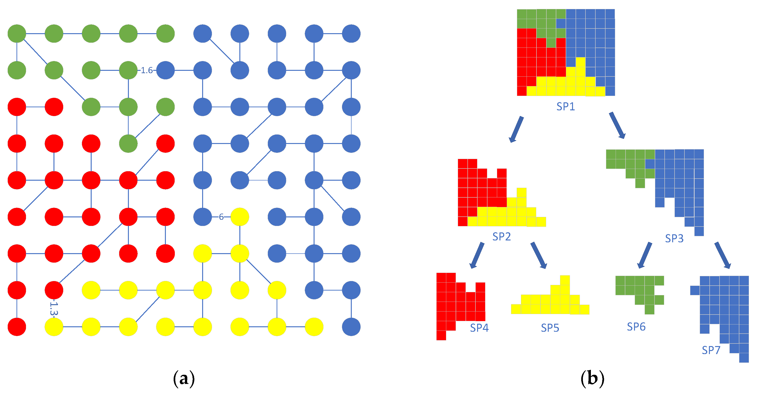
2.3. Hierarchical Segmentation

Let $G=(V,E)$ be an undirected graph. $V=\{v_1,v_2,\dots ,v_n\}$ are vertices of the graph and they are locally connected with its neighbor (constructed by 8-neighborhood), and n is the number of vertices. $E=\{e_1,e_2,\dots ,e_m\}$ are weighted edges and $e=(u,v)$ is a non-negative value that measures the dissimilarity between vertex $u$ and $v$, and $m$ is the count of edges.

Our method based on the Boruvka algorithm can construct a minimum spanning tree (MST) from the bottom up, and it is a type of merging method. At first, all the pixels of the PolSAR image are initialized as an isolated MST. For each MST, we search the nearest neighbors in 8 directions and connect them together

$$D(MS{T}_1,MS{T}_2)=\underset{u\in MS{T}_1,v\in MS{T}_2,w(u,v)\in E}{\min }w(u,v).$$

(20)

As explained in Section 3.1, we can measure the distance between two MSTs with formula (19). After each iteration of the search, all the features of the old MSTs are aggregated into the new one. Then, all the weights of the outgoing edges are updated through cutting the self-loop and preserving the lightest one.

The MST merging operation uses a deep-first search based on the greedy strategy, and the edges with small edge weights are merged early in the iteration procedure. During each merging iteration, each MST merges at least one neighbor MST and the number of MSTs decreases by at least half of the original one. Finally, there is one MST left. The Boruvka algorithm obtains the local optimal solution and has the advantage of parallel processing with low time complexity.

Based on the obtained MST structure, superpixels can be generated by splitting the MST into sub-MSTs. Figure 2 presents a brief explanation of PolSAR image segmentation under the MST structure. The preset number of superpixels is 4. The final MST structure is shown in Figure 2a, and the PolSAR image is considered as one superpixel right now. The blue lines denote edges between different trees. It is worth noting that all the weights of the edges that do not display values are smaller than 1.3. For all the edges in this MST, the edge with largest weight is found, i.e., 6, and it is cut. One MST splits into two new ones. The edge sorting is redone in a descending order within each new MST and the edges with largest weights 1.3 and 1.6 are removed. There are 4 sub-MSTs left and 4 superpixels are generated. The superpixel segmentation process is shown in Figure 2b. As we can see, the superpixel SP1 is composed of SP2 and SP3 and the superpixel SP2 generates SP4 and SP5. The coarser level superpixels are composed of finer level superpixels, demonstrating the hierarchical property of the MST. Therefore, we can generate any number of superpixels by cutting edges in descending order of weights.

2.4. Implementation Details

So far, the hierarchical superpixel segmentation method based on MST is completed and the implementation details are provided as follows. Assume there are N pixels in a PolSAR image, and K superpixels are expected. Each pixel is initialized as one MST. Subsequently, the isolated MSTs are merged with their nearest neighboring MSTs until one MST is left according to (19). The more dissimilar the two regions in the image are, the greater the edge weight between the subtrees in the corresponding MST. Next, the edges are sorted in descending order of weights and the top K-1 largest edges are cut. There are K sub-MSTs left, representing K superpixels in the PolSAR image. The detailed segmentation steps are listed in Algorithm 1.

Algorithm 1. Superpixel generation for the PolSAR image.

Input: The original PolSAR image and the predetermined number of superpixels K.

Output: The average image of the segmentation results.

1. Each pixel is initialized as an MST, and the RFCD feature, edge map, ENL map, and Homogeneity map are calculated.

2. Traverse the table of edges to find the tree closest to each tree by calculating weight using (19), and connect them, obviously, the number of trees is halved.

3. Repeat step 2 until there is one tree left, which is the final MST.

4. Sort the edges in each MST according to the weight in descending order.

5. Cut off the edge with largest weight to obtain new MSTs.

6. If the number of MSTs is equal to K, average the pixel value in each MST. Or repeat steps 4 and 5.

7. Output the average image of the segmentation results.

Once the MST is constructed, it does not need to be reconstructed for different levels of segmentation, which saves a lot of time compared to other algorithms. Based on this structure, we can obtain any amount of superpixels in real time. The superpixels at a coarse level are composed of fine level superpixels, and the local image details are preserved to the greatest extent. The whole schematic concept of our method is presented in Figure 3.

3. Experimental Results and Analysis

3.1. Dataset Description and Parameter Setting

To verify the segmentation accuracy and efficiency of our proposed method, two fully polarimetric images are adopted in the following experiments. The first PolSAR image is acquired from the ESAR L-band system, in Oberpfaffenhofen, Germany. The size of the image is 1117 × 934 with the resolution of 1.50 m × 1.8 m (azimuth × range). This area contains both homogeneous areas (such as roads and farmlands) and heterogeneous areas (such as urban buildings and forests). The second area is located in Elpaso, USA. It is acquired using an AIRSAR L-band system and consists of 545 × 545 pixels with the resolution of 5.0 m × 2.8 m (azimuth × range). It also includes complex urban buildings, streets, and plain farmlands. These PolSAR data are all single look. Figure 4 presents the pseudo-color images of Pauli decomposition of these two datasets.

Two superpixel segmentation algorithms, namely, the Pol-ASLIC in [19] and the Pol-ERM in [26], are used for comparison in the experiments. Xiang and Wang modified the original SLIC method and ER method and achieved good performance in PolSAR imagery. To ensure objectivity, the parameter settings of these two methods are consistent with those in the paper. Regarding our proposed method, the parameter ${\sigma }_C$ in (19) is manually set to 0.1 and $S_{TH}$ is set to 3. The parameters $\alpha$, ${\sigma }_x$, and $\beta$ of the edge detector are set to 2, 2, and 1.25, respectively.

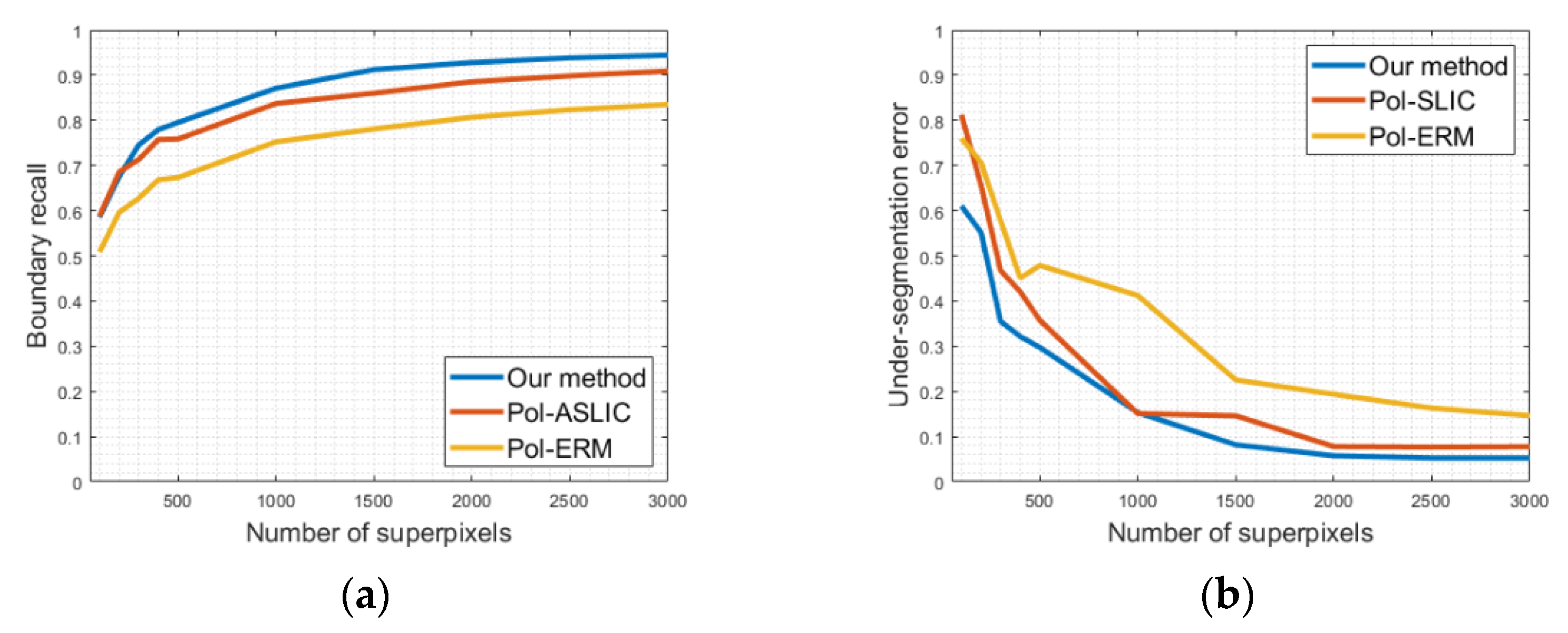
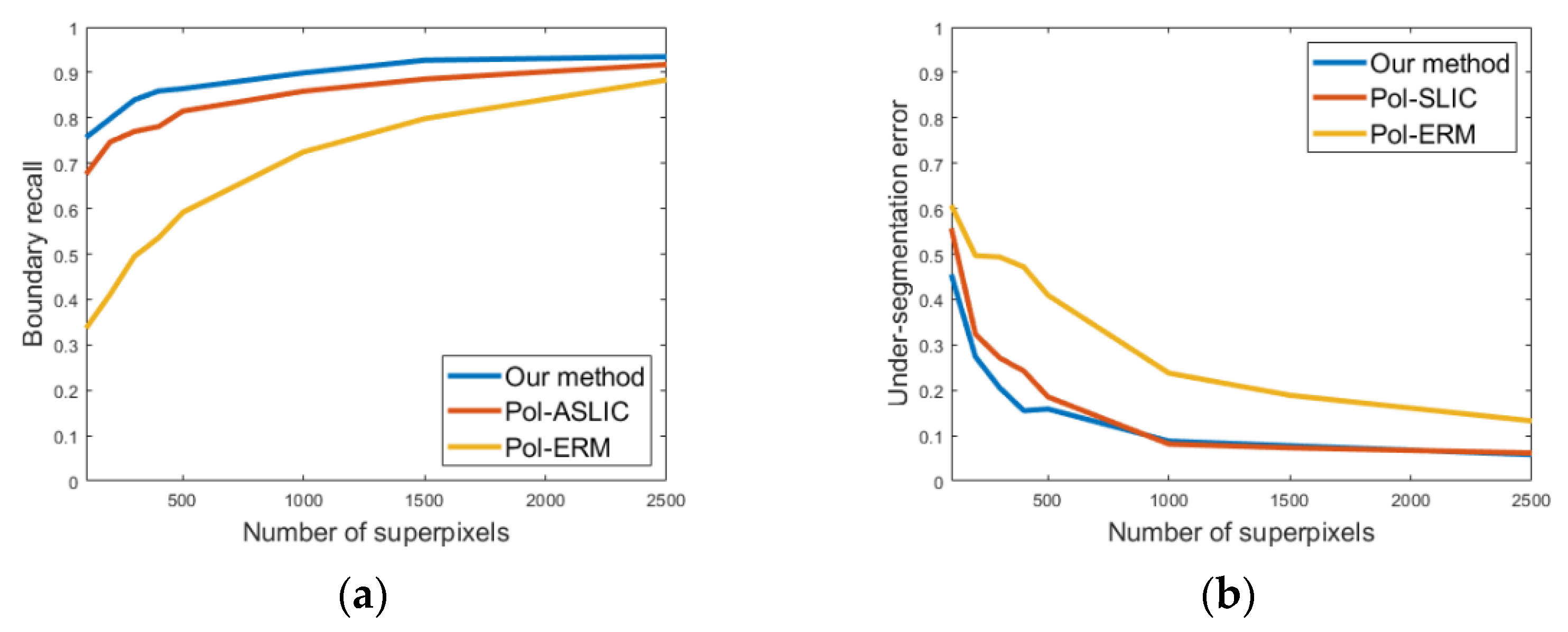
3.2. Quantitative Evaluation Metrics

To further evaluate the performance of our method besides qualitative visual assessment, we chose two metrics used in [26], i.e., boundary recall (BR) and under-segmentation error (UE). The boundary recall (BR) measures the percentage of ground truth edge pixels that fall within superpixel boundary pixels and is defined as

$$BR=\frac{TP}{TP+FN},$$

(21)

where TP is the number of superpixels boundary pixels falling in the true edge and FN is the opposite case. The margin is set to 2, which indicates that a superpixel boundary pixel within two pixels of the true boundary can be considered as correctly covered. Thus, a high BR means the superpixels can adhere well to the image boundaries. The under-segmentation error measures the percentage of pixels of superpixels that leak across the ground truth object edge. It is defined as

$$UE=\frac{{\displaystyle {\sum }_i{\displaystyle {\sum }_k\min (S(s_k\cap g_i),S(s_k-g_i))}}}{{\displaystyle {\sum }_{i}S(g_i)}},$$

(22)

where $g_i$ is a ground true object, $s_k$ is a superpixel, and S(∙) denotes the number of segment pixels. A lower UE value denotes that the superpixel boundaries adhere to the objects’ edges in the image and few pixels exceed the real edges.

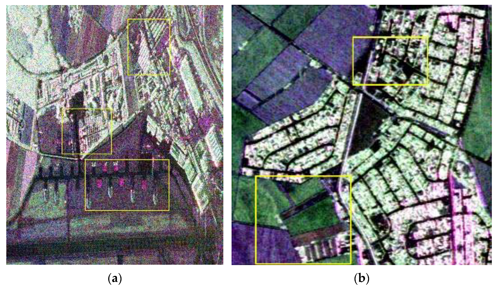
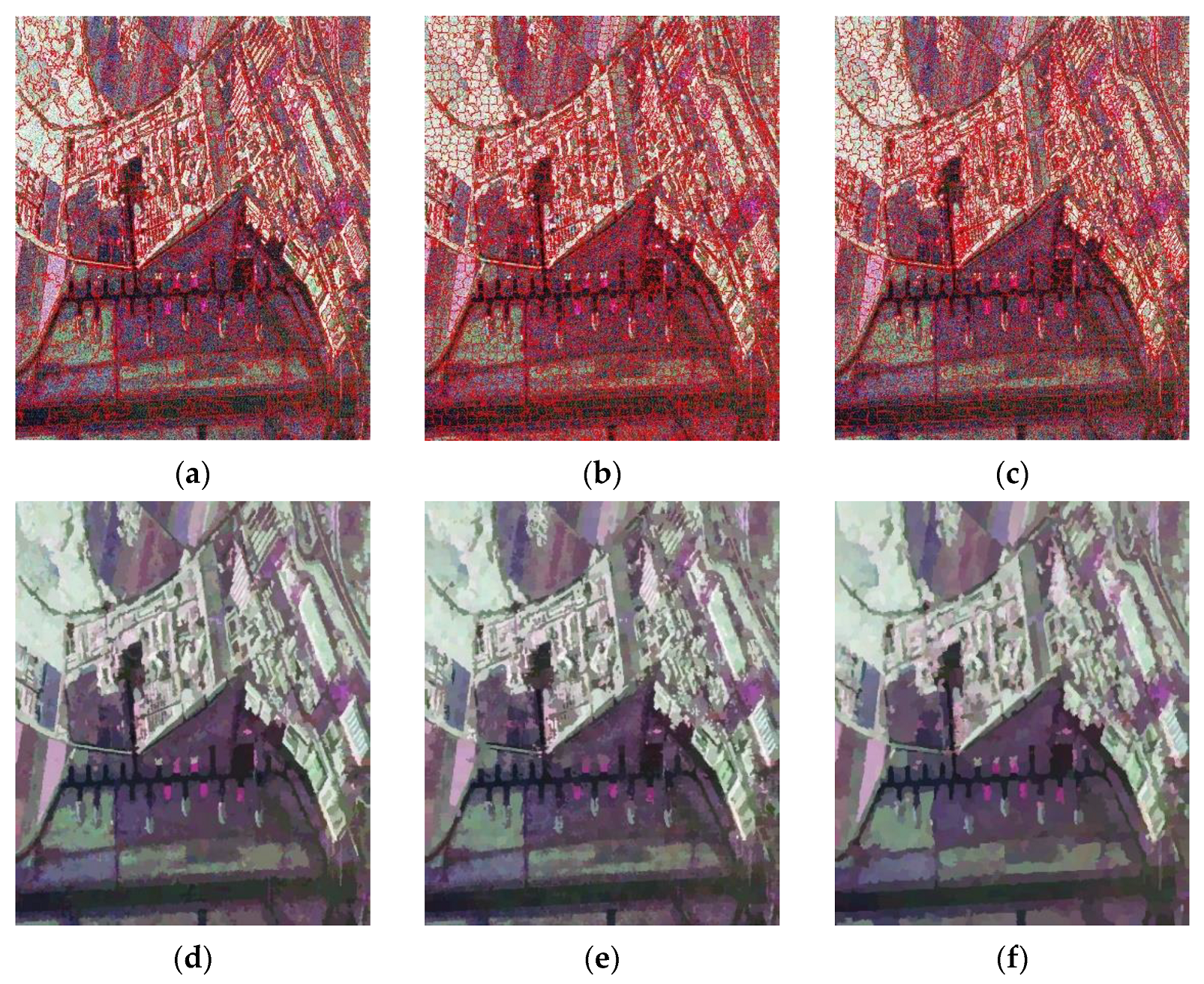
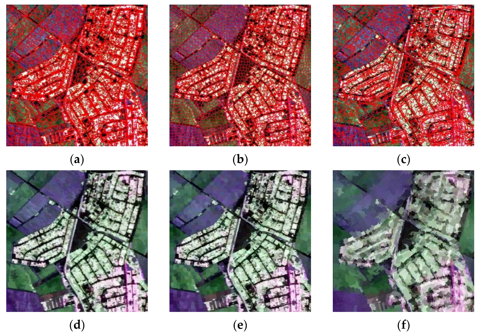
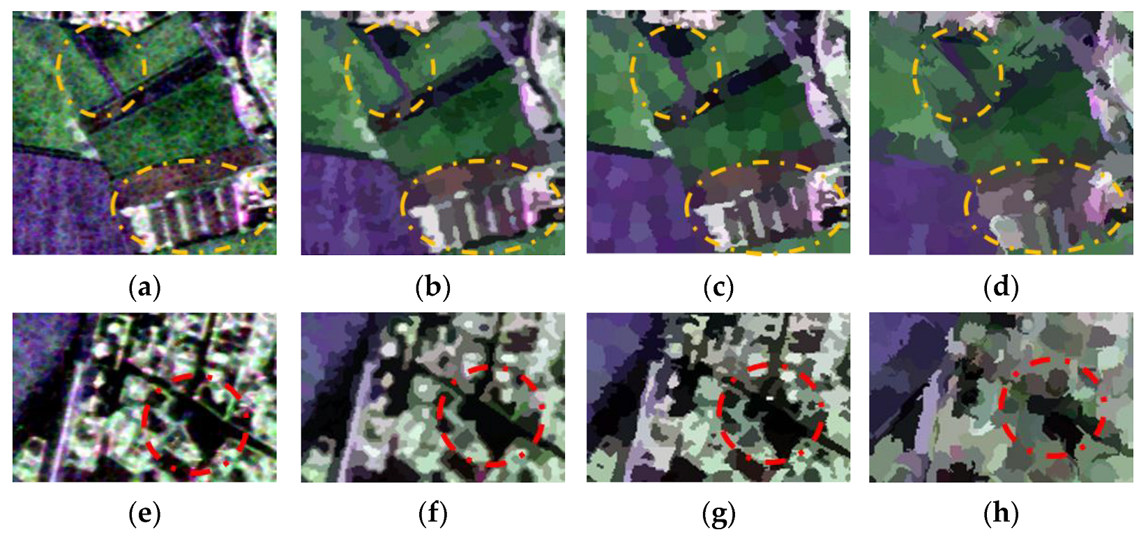
3.3. Superpixel Segmentation Results of ESAR Data

The Figure 5 presents the superpixel segmentation results of ESAR data using the proposed method, the Pol-ASLIC and the Pol-ERM, respectively, while the number of superpixels is set to 2500. The first row shows the edges of the superpixel and the red lines depict the boundaries. The results of Pol-ASLIC and Pol-ERM have similar segment sizes. The superpixel size of the proposed method is adaptive according to the local polarimetric information. The segment size becomes larger in the homogeneous regions and the opposite in the heterogeneous areas. The second row presents the superpixels with their covariance matrix averaged. From a global perspective, the segmentation performance of the three methods is pretty good. To obtain a more vivid visual inspection, three patches in Figure 4a marked by yellow rectangles are enlarged in Figure 6 for a more granular comparison.

The original local region and the segmentation results of the three methods are shown side-by-side in Figure 6. Compared with the original image, most of the boundaries and built-up areas are well preserved by our method. Look at the first row of Figure 6a–d, such as the green ribbon architectural details in the upper right corner, only the segmentation results of our method are well preserved. In the dense natural area such as Figure 6e, thanks to the decomposed scattering mechanism information and edge information, our method lost the least local shape information, which can be easily seen in the small regions highlighted by green arrows and marked by red ellipses. Another reason for the good performance is that the model of MST contains hierarchical structure information. Since the spatial distance is not considered in our algorithm, the more local details the region has, the denser and more compact the superpixels are. The clustering-based methods may lose local details due to the predefined cluster seed, although they are already in the gradient minimum region. Additionally, the SIRV model is not suitable for natural areas. Figure 6i–l highlights the importance of homogeneity and edge information because the homogeneous regions look smooth and the edges of the objects are fine in Figure 6j.

Figure 7 shows the BR and UE curves of the three methods, respectively, when the superpixel number ranges from 100 to 3000. The Pol-ERM has the worst performance while our method outperforms others. This is because the fine five-component decomposition results enable the algorithm to distinguish different classes of objects locally, and the edge strength map and homogeneity metrics enable the large-scale superpixels to maintain good edge adhesion.

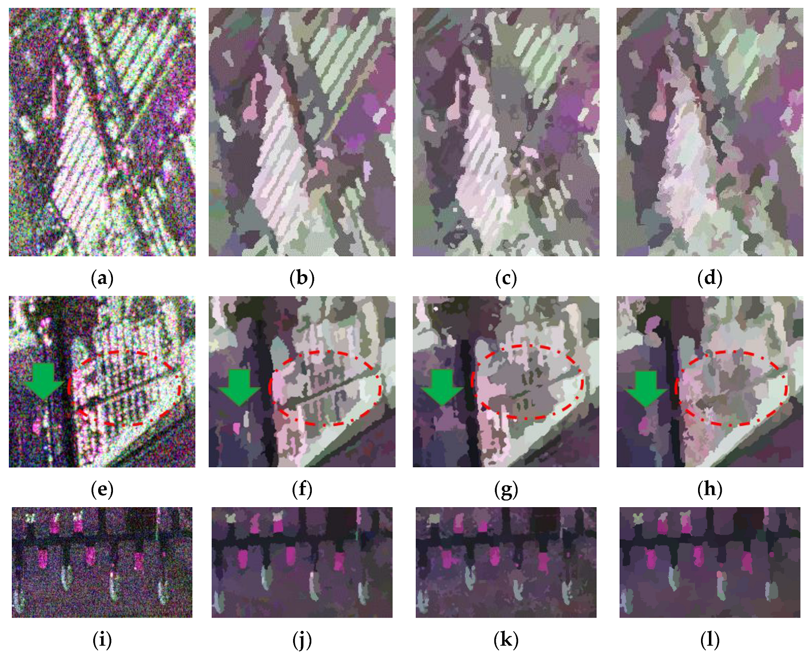
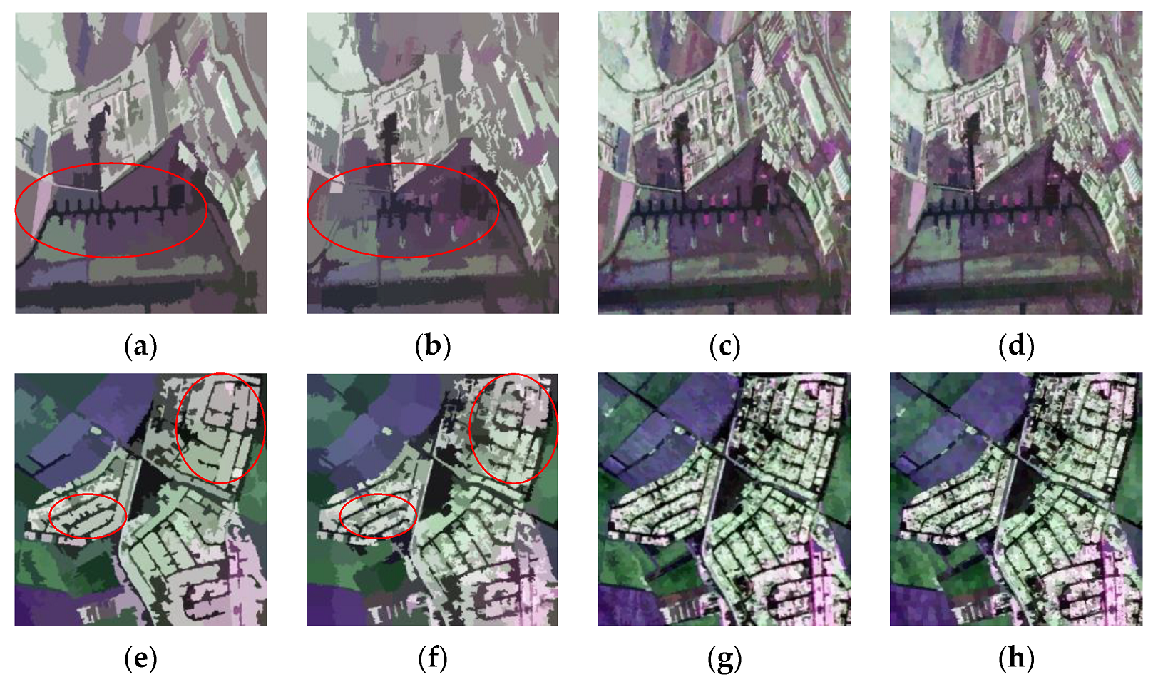
3.4. Superpixel Segmentation Results of AIRSAR Data

Figure 8 shows the superpixel results of AIRSAR data using the proposed methods Pol-ASLIC and Pol-ERM, with the number set to 2500. Figure 8a–c shows the image with edges of superpixels and Figure 8d–f presents the averaged results. As shown in Figure 8d–f, from the global perspective, our method and the Pol-ASLIC perform better in the object-dense regions. The Pol-ASLIC easily obtains more regular superpixels due to its clustering framework and spatial constraint. Additionally, the shape of most natural landscapes is rectangle-like, making the Pol-ASLIC method very suitable in homogeneous areas. Since the Pol-ERM only takes limited polarimetric information, the shape of the results is not very close to the real objects.

From Figure 9a–d, our method significantly outperforms the others. In the top left ellipse, the straight road is well preserved in Figure 9b, while the one in Figure 9c becomes bent and the one in Figure 9d is deformed. In the dotted orange ellipse in the lower right corner, the details of the white bar objects are well preserved by our method. The edge structure is lost in Figure 9g–h, while it is preserved in Figure 9f. From the view of both the global segmentation performance and the preservation of local details, our algorithm outperforms others. The global properties are captured due to the edge penalty and homogeneity constraint, and the local details are well preserved because of the scattering features produced by the RFCD results. The curves of BR and UE shown in Figure 10a–b also quantitatively demonstrate the superiority of the proposed method. The UE curve of Pol-ASLIC almost coincides with that of ours in the 1000 and 3000 range, but the better under-segmentation error curve means that the MST structure still outperforms the regular sampling strategy of the SLIC scheme.

4. Discussion

4.1. Multi-Scale Comparison

To highlight the advantages of our method in multi-scale segmentation, the superpixel results of the proposed method and Pol-ASLIC are assessed in Figure 11, when the segmentation scale is 100 and 2500. Apparently, the results derived from our method are close to the human vision system both at small scale (K=100) and at large scale (K = 2500). The results of Pol-ASLIC lose local structure in some places at small scales. As we can see in these red oval boxes in Figure 11a–b, the outline of the road becomes blurred in Figure 11b and the opposite in Figure 11a. The differences in details of the different methods can also be seen very clearly in Figure 11e-f. The edges of objects in Figure 11a,e are smoother than those in Figure 11b,f, which demonstrates advantages in segmentation accuracy of our method at small scales. Moreover, the advantages of the proposed method at large scales are clarified in Section 3.3 and Section 3.4. The proposed method can maintain good segmentation performance at multiple scales, visually.

Our hierarchical method will preserve global frameworks at small scales and show local details at large scales. This is because we generate superpixels based on the unity framework of the MST structure. As we can see in Figure 12, the 50, 100, and 500 superpixels generated by our method are presented in order. The yellow edges in Figure 12a are boundaries of 50 superpixel boundaries and the yellow edges in Figure 12b are exactly the same as Figure 12a. It can be seen that when the superpixel number changes from 50 to 100, the segmentation is further performed on the basis of 50 superpixels. Additionally, finer local details are obtained within the original boundaries according to the coarser level of superpixels. When the superpixel number is increased to 500, more image details are subdivided within the original 100 superpixel results in Figure 12c. It shows that large-sized superpixels are composed of smaller ones, which demonstrates that our algorithm is hierarchical. This property enables our method to reduce the computation time with better boundary preservation when undertaking multiscale tasks.

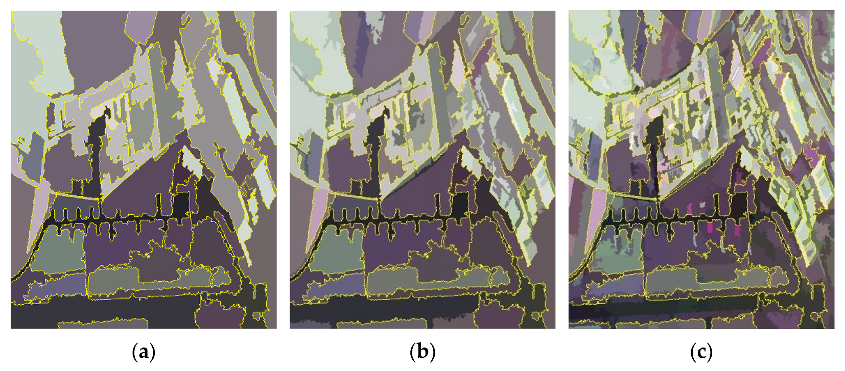
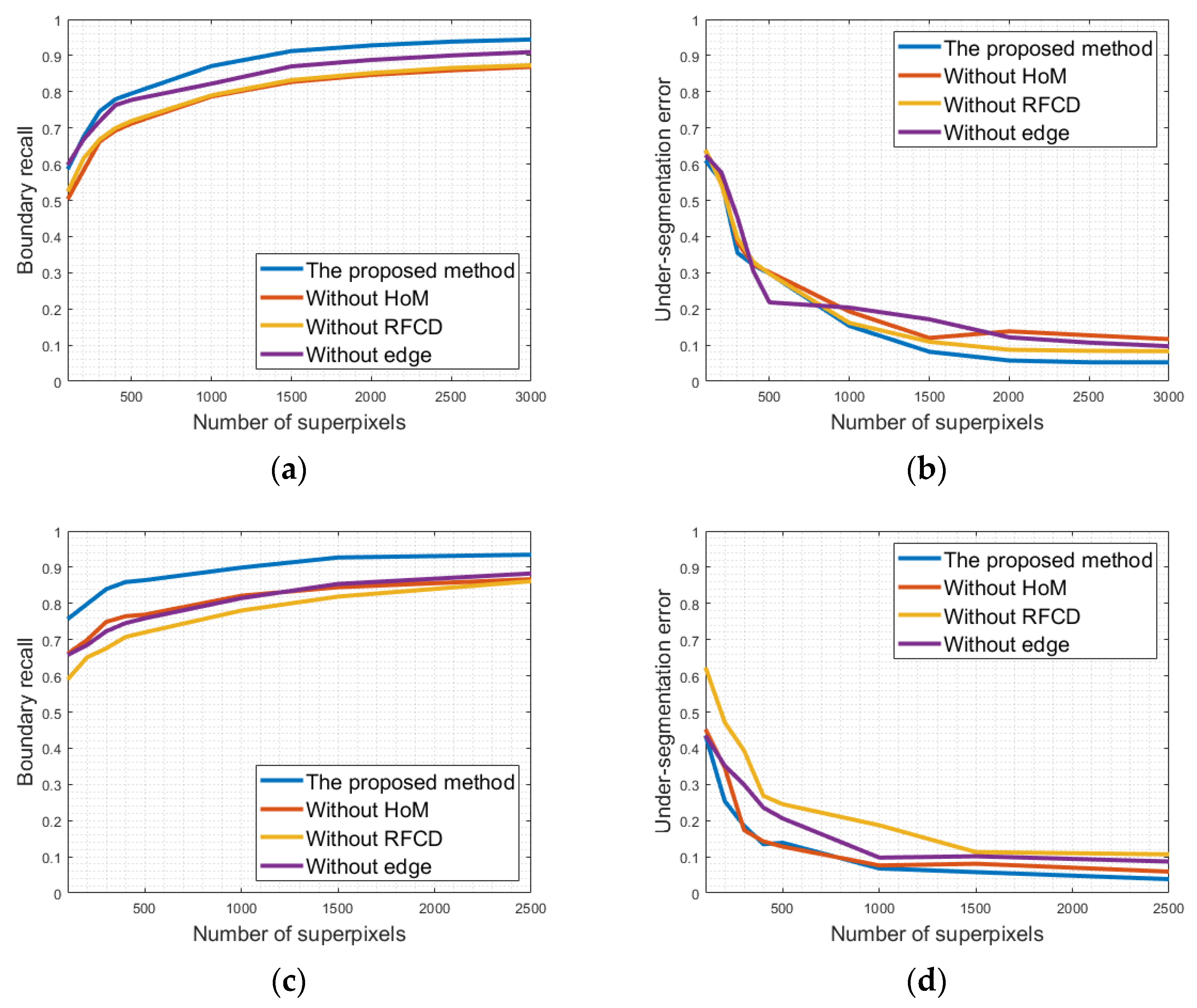
4.2. Contribution Analysis of the Distances Measure

The distance measure of our method combines the scattering mechanism distance, edge enhancement factor, and homogeneity information. The RFCD feature had great physical scattering interpretation in the superpixel segmentation. Additionally, we chose it as the basis for the distance metric. The edge information that describes the structural details in the image is beneficial for improving the segmentation accuracy. It can help to enlarge the distance between pixels falling on the edge and can help preserve the boundary adherence of generated superpixels. In addition, the homogeneity measure is also applied to make pixels in homogeneous regions more likely to form a superpixel. To determine which feature contributes the most in the proposed method, we conducted segmentation accuracy analysis on the results from the proposed algorithm with or without these dissimilarity measures. Figure 13 presents the BR and UE curves based on ESAR and AIRSAR data sets. It can be seen that in both datasets the original proposed method has the highest BR and lowest UE, which demonstrates the effectiveness of all these selected distance metrics. After removing the scattering mechanism distance derived from RFCD, the performance of BR and UE dropped the most, which denotes that it plays a key role in maintaining segmentation accuracy. According to the curves of method without the edge enhancement factor or homogeneity distance in Figure 13a–c, the homogeneity distance seems to contribute more than the edge enhancement factor to some extent, but not as significant as RFCD. Hence, we can conclude that the proposed distance measure is useful for the segmentation algorithm and the RFCD contributes the most.

4.3. Computational Complexity and Run Time

The framework of Pol-ASLIC is consistent with SLIC, and SLIC is a method based on k-means local clustering within a region. Assume the number of the pixels in the image is n. The computational complexity of Pol-ASLIC is $O(n)$ in each iteration but it needs several iterations. The Pol-ERM has a similar framework to the ERS approach. It is a graph-based method and the main procedure is selecting a subset of edges by optimizing a clustering function. The optimization is solved with a greedy algorithm, so the worst complexity is $O(n^2\log n)$ while its average complexity is $O(n\log n)$. Our method is based on the Boruvka algorithm and it has been proven [28] that it takes $O(n)$ to construct the MST and segment it.

The time–cost comparison of different methods based on ESAR and AIRSAR datasets is shown in

Table 1. Time–cost of different superpixel generation methods for two PolSAR datasets (seconds).

Methods	Datasets	Number of Superpixels				Average
		500	1000	2500	5000
The proposed method	ESAR	3.912	3.931	3.896	3.895	3.909
	AIRSAR	1.068	1.066	1.073	1.072	1.070
Pol-ASLIC	ESAR	12.709	15.292	10.297	15.487	13.446
	AIRSAR	12.868	21.523	17.049	13.832	16.318
Pol-ERM	ESAR	12.344	14.016	20.578	31.266	19.551
	AIRSAR	4.281	5.125	7.313	9.328	6.512

. All the experiments were executed on a desktop with AMD Ryzen 5 4600H of 3.00 GHz and 16 GB memory. We did not use any parallelization (multi-core or GPU). The run-time of Pol-ASLIC is much greater than that of ours and fluctuates within a certain range, which is influenced by a local clustering procedure. The speed of Pol-ERM is almost six times slower than the proposed method, and the time increases with respect to the number of segments. Our method uses the least amount of time and is almost independent of the segmentation scale. Since all scales of superpixels are generated from the same one MST, our algorithm can generate superpixels at all scales in real time.

4.4. Analysis of the Limitation

The results and analysis of the sections above prove that the proposed method outperforms two other state-of-the-art methods in both qualitative and quantitative manners. However, there are many visually unsatisfactory superpixel results that are irregular in homogeneous areas, such as the farmland in Figure 8a. One of the reasons is that the utilized RFCD feature extraction is overly fine and the over-segmentations appear. From another point of view, the superpixels may grow diversely in different directions (MST construction process) inside the homogeneous areas, since there is no spatial constraint like the SLIC method. However, it does not affect the quantitative segmentation performance because the irregular results always appear inside the ground truth object. The similarity metric of the proposed method can be improved if more spatial and texture information is introduced. In addition, the parameter σ in formula (19) is set manually, which cannot adaptively adjust the weight of homogeneity measurement $D_H$. This can be improved by adaptive selection of parameters left in future work.

5. Conclusions

In this paper, we proposed a robust hierarchical superpixel segmentation method for PolSAR images, utilizing the minimum spanning tree algorithm. The refined five-component polarimetric decomposition feature was used to construct a distance that measures the dissimilarity between neighboring pixels. In addition, the edge enhancement factor calculated by exploiting the statistical information in PolSAR data was utilized to help maintain edge adhesion. A homogeneity measurement was also used to further improve the segmentation accuracy. After generating the MST structure for the PolSAR image, the hierarchical segmentation was performed based on the dissimilarities. Thanks to the unified hierarchical tree framework, the superpixels at coarse level were composed of ones at finer levels, and the segmentation results of different scales were visually close to the original image. In addition, the segmentation time was very fast. Experiments based on ESAR and AIRSAR data demonstrate that the performance of the proposed method surpassed the state-of-the-art algorithm, from the perspective of segmentation accuracy and time efficiency. We will utilize this method for ship-detection research in the future. In addition, the acceleration of edge information computing and the adaptive setting of the parameters are also worthy of attention.

References

- Liu, S.J.; Luo, H.; Shi, Q. Active Ensemble Deep Learning for Polarimetric Synthetic Aperture Radar Image Classification. IEEE Geosci. Remote Sens. Lett. 2021, 18, 1580–1584. [Google Scholar] [CrossRef]
- Imani, M. Median-mean line based collaborative representation for PolSAR terrain classification. Egypt. J. Remote Sens. Space Sci. 2022, 25, 281–288. [Google Scholar] [CrossRef]
- Jiang, Y.; Li, M.; Zhang, P.; Tan, X.; Song, W. Unsupervised Complex-Valued Sparse Feature Learning for PolSAR Image Classification. IEEE Trans. Geosci. Remote Sens. 2022, 60, 1–16. [Google Scholar] [CrossRef]
- Ni, J.; Xiang, D.; Lin, Z.; López-Martínez, C.; Hu, W.; Zhang, F. DNN-Based PolSAR Image Classification on Noisy Labels. IEEE J. Sel. Top. Appl. Earth Obs. Remote Sens. 2022, 15, 3697–3713. [Google Scholar] [CrossRef]
- Cui, X.C.; Su, Y.; Chen, S.W. A Saliency Detector for Polarimetric SAR Ship Detection Using Similarity Test. IEEE J. Sel. Top. Appl. Earth Obs. Remote Sens. 2019, 12, 3423–3433. [Google Scholar] [CrossRef]
- Cheng, J.; Zhang, F.; Xiang, D.; Yin, Q.; Zhou, Y. PolSAR Image Classification with Multiscale Superpixel-Based Graph Convolutional Network. IEEE Trans. Geosci. Remote Sens. 2022, 60, 1–14. [Google Scholar] [CrossRef]
- Zhang, T.; Wang, W.; Quan, S.; Yang, H.; Xiong, H.; Zhang, Z.; Yu, W. Region-Based Polarimetric Covariance Difference Matrix for PolSAR Ship Detection. IEEE Trans. Geosci. Remote Sens. 2022, 60, 1–16. [Google Scholar] [CrossRef]
- Zhang, T.; Du, Y.; Yang, Z.; Quan, S.; Liu, T.; Xue, F.; Chen, Z.; Yang, J. PolSAR Ship Detection Using the Superpixel-Based Neighborhood Polarimetric Covariance Matrices. IEEE Geosci. Remote Sens. Lett. 2022, 19, 1–5. [Google Scholar] [CrossRef]
- Achanta, R.; Shaji, A.; Smith, K.; Lucchi, A.; Fua, P.; Süsstrunk, S. SLIC Superpixels Compared to State-of-the-Art Superpixel Methods. IEEE Trans. Pattern Anal. Mach. Intell. 2012, 34, 2274–2282. [Google Scholar] [CrossRef]
- Jianbo, S.; Malik, J. Normalized cuts and image segmentation. IEEE Trans. Pattern Anal. Mach. Intell. 2000, 22, 888–905. [Google Scholar] [CrossRef]
- Chen, J.; Li, Z.; Huang, B. Linear Spectral Clustering Superpixel. IEEE Trans. Image Processing 2017, 26, 3317–3330. [Google Scholar] [CrossRef]
- Comaniciu, D.; Meer, P. Mean shift: A robust approach toward feature space analysis. IEEE Trans. Pattern Anal. Mach. Intell. 2002, 24, 603–619. [Google Scholar] [CrossRef]
- Qin, F.; Guo, J.; Lang, F. Superpixel Segmentation for Polarimetric SAR Imagery Using Local Iterative Clustering. IEEE Geosci. Remote Sens. Lett. 2015, 12, 13–17. [Google Scholar] [CrossRef]
- Song, H.; Yang, W.; Bai, Y.; Xu, X. Unsupervised classification of polarimetric SAR imagery using large-scale spectral clustering with spatial constraints. Int. J. Remote Sens. 2015, 36, 2816–2830. [Google Scholar] [CrossRef]
- Feng, J.; Cao, Z.; Pi, Y. Polarimetric Contextual Classification of PolSAR Images Using Sparse Representation and Superpixels. Remote Sens. 2014, 6, 7158–7181. [Google Scholar] [CrossRef]
- Xu, Q.; Chen, Q.; Yang, S.; Liu, X. Superpixel-Based Classification Using K Distribution and Spatial Context for Polarimetric SAR Images. Remote Sens. 2016, 8, 619. [Google Scholar] [CrossRef]
- Hou, B.; Yang, C.; Ren, B.; Jiao, L. Decomposition-Feature-Iterative-Clustering-Based Superpixel Segmentation for PolSAR Image Classification. IEEE Geosci. Remote Sens. Lett. 2018, 15, 1239–1243. [Google Scholar] [CrossRef]
- Zhang, L.; Han, C.; Cheng, Y. Improved SLIC superpixel generation algorithm and its application in polarimetric SAR images classification. In Proceedings of the 2017 IEEE International Geoscience and Remote Sensing Symposium (IGARSS), Fort Worth, TX, USA, 23–28 July 2017; pp. 4578–4581. [Google Scholar]
- Xiang, D.; Ban, Y.; Wang, W.; Su, Y. Adaptive Superpixel Generation for Polarimetric SAR Images With Local Iterative Clustering and SIRV Model. IEEE Trans. Geosci. Remote Sens. 2017, 55, 3115–3131. [Google Scholar] [CrossRef]
- Lin, H.; Bao, J.; Yin, J.; Yang, J. Superpixel Segmentation with Boundary Constraints for Polarimetric SAR Images. In Proceedings of the IGARSS 2018—2018 IEEE International Geoscience and Remote Sensing Symposium, Valencia, Spain, 22–27 July 2018; pp. 6195–6198. [Google Scholar]
- Quan, S.; Xiang, D.; Wang, W.; Xiong, B.; Kuang, G. Scattering Feature-Driven Superpixel Segmentation for Polarimetric SAR Images. IEEE J. Sel. Top. Appl. Earth Obs. Remote Sens. 2021, 14, 2173–2183. [Google Scholar] [CrossRef]
- Xu, X.; Zou, B.; Zhang, L. Polarimetric Semivariogram-Based Spatial Scale Selection for PolSAR Image Segmentation with Mean-Shift Algorithm. IEEE Geosci. Remote Sens. Lett. 2020, 18, 1239–1243. [Google Scholar] [CrossRef]
- Lang, F.; Yang, J.; Yan, S.; Qin, F. Superpixel Segmentation of Polarimetric Synthetic Aperture Radar (SAR) Images Based on Generalized Mean Shift. Remote Sens. 2018, 10, 1592. [Google Scholar] [CrossRef]
- Liu, B.; Hu, H.; Wang, H.; Wang, K.; Liu, X.; Yu, W. Superpixel-Based Classification With an Adaptive Number of Classes for Polarimetric SAR Images. IEEE Trans. Geosci. Remote Sens. 2013, 51, 907–924. [Google Scholar] [CrossRef]
- Xu, X.; Zou, B.; Zhang, L. Object-based Normalized-Cuts for High-Resolution Polsar Image Segmentation. In Proceedings of the 2019 SAR in Big Data Era (BIGSARDATA), Beijing, China, 5–6 August 2019; pp. 1–4. [Google Scholar]
- Wang, W.; Xiang, D.; Ban, Y.; Zhang, J.; Wan, J. Superpixel Segmentation of Polarimetric SAR Images Based on Integrated Distance Measure and Entropy Rate Method. IEEE J. Sel. Top. Appl. Earth Obs. Remote Sens. 2017, 10, 4045–4058. [Google Scholar] [CrossRef]
- Lin, W.; Li, Y. Parallel Regional Segmentation Method of High-Resolution Remote Sensing Image Based on Minimum Spanning Tree. Remote Sens. 2020, 12, 783. [Google Scholar] [CrossRef]
- Wei, X.; Yang, Q.; Gong, Y.; Ahuja, N.; Yang, M.H. Superpixel Hierarchy. IEEE Trans Image Process 2018, 27, 4838–4849. [Google Scholar] [CrossRef]
- Zhang, W.; Xiang, D.; Su, Y. Fast Multiscale Superpixel Segmentation for SAR Imagery. IEEE Geosci. Remote Sens. Lett. 2022, 19, 1–5. [Google Scholar] [CrossRef]
- Wang, W.; Xiang, D.; Ban, Y.; Zhang, J.; Wan, J. Enhanced edge detection for polarimetric SAR images using a directional span-driven adaptive window. Int. J. Remote Sens. 2018, 39, 6340–6357. [Google Scholar] [CrossRef]
- Xiang, D.; Ban, Y.; Wang, W.; Tang, T.; Su, Y. Edge Detector for Polarimetric SAR Images Using SIRV Model and Gauss-Shaped Filter. IEEE Geosci. Remote Sens. Lett. 2016, 13, 1661–1665. [Google Scholar] [CrossRef]
- Quan, S.; Xiong, B.; Xiang, D.; Hu, C.; Kuang, G. Scattering Characterization of Obliquely Oriented Buildings from PolSAR Data Using Eigenvalue-Related Model. Remote Sens. 2019, 11, 581. [Google Scholar] [CrossRef]
- Wang, W.; Zhai, Q.; Ban, Y.; Zhang, J.; Wan, J. PolSAR image segmentation based on hierarchical region merging and segment refinement with WMRF model. In Proceedings of the 2017 IEEE International Geoscience and Remote Sensing Symposium (IGARSS), Fort Worth, TX, USA, 23–28 July 2017; pp. 4574–4577. [Google Scholar]
- Goodman, N.R. Statistical Analysis Based on a Certain Multivariate Complex Gaussian Distribution (An Introduction). Ann. Math. Stat. 1963, 34, 152–177. [Google Scholar] [CrossRef]
- Conradsen, K.; Nielsen, A.A.; Schou, J.; Skriver, H. A test statistic in the complex wishart distribution and its application to change detection in polarimetric SAR data. IEEE Trans. Geosci. Remote Sens. 2003, 41, 4–19. [Google Scholar] [CrossRef]
- Yamaguchi, Y.; Moriyama, T.; Ishido, M.; Yamada, H. Four-component scattering model for polarimetric SAR image decomposition. IEEE Trans. Geosci. Remote Sens. 2005, 43, 1699–1706. [Google Scholar] [CrossRef]
- Quan, S.; Xiong, B.; Xiang, D.; Zhao, L.; Zhang, S.; Kuang, G. Eigenvalue-Based Urban Area Extraction Using Polarimetric SAR Data. IEEE J. Sel. Top. Appl. Earth Obs. Remote Sens. 2018, 11, 458–471. [Google Scholar] [CrossRef]
- Yu, W.; Wang, Y.; Liu, H.; He, J. Superpixel-Based CFAR Target Detection for High-Resolution SAR Images. IEEE Geosci. Remote Sens. Lett. 2016, 13, 730–734. [Google Scholar] [CrossRef]
- Lang, F.; Yang, J.; Li, D. Adaptive-Window Polarimetric SAR Image Speckle Filtering Based on a Homogeneity Measurement. IEEE Trans. Geosci. Remote Sens. 2015, 53, 5435–5446. [Google Scholar] [CrossRef]
- Liu, B.; Zhang, Z.; Liu, X.; Yu, W. Edge Extraction for Polarimetric SAR Images Using Degenerate Filter with Weighted Maximum Likelihood Estimation. IEEE Geosci. Remote Sens. Lett. 2014, 11, 2140–2144. [Google Scholar] [CrossRef]
- Anfinsen, S.N.; Doulgeris, A.P.; Eltoft, T. Estimation of the Equivalent Number of Looks in Polarimetric Synthetic Aperture Radar Imagery. IEEE Trans. Geosci. Remote Sens. 2009, 47, 3795–3809. [Google Scholar] [CrossRef]