
Integrated Radar and Communications Waveform Design Based on Multi-Symbol OFDM


Abstract
:
1. Introduction
2. Multi-Symbol OFDM-Based IRC Systems and Signal Model
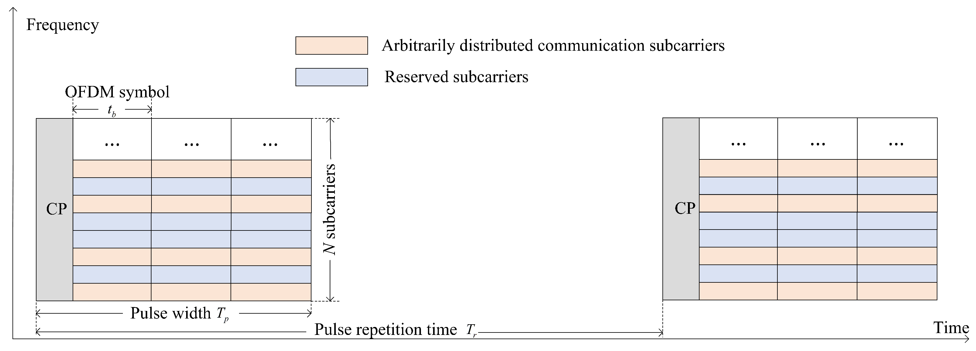
2.1. Multi-Symbol OFDM-Based IRC Signal Model
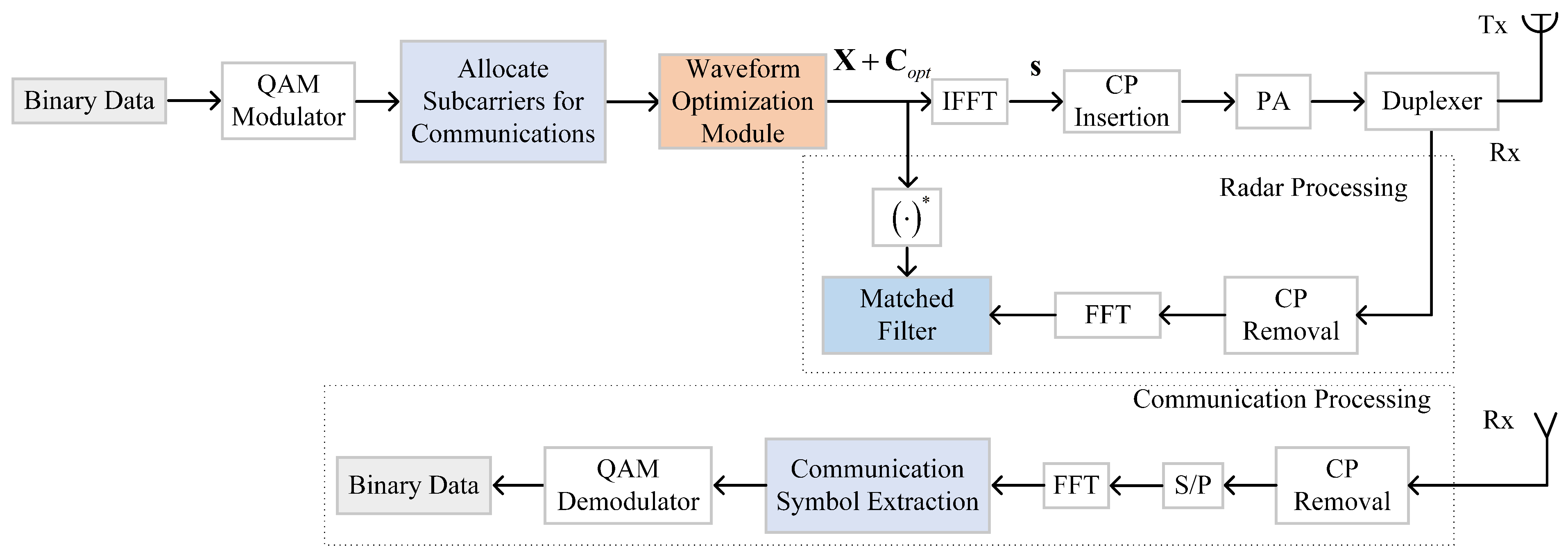
2.2. Multi-Symbol OFDM-Based IRC System
3. IRC Waveform Design Objective
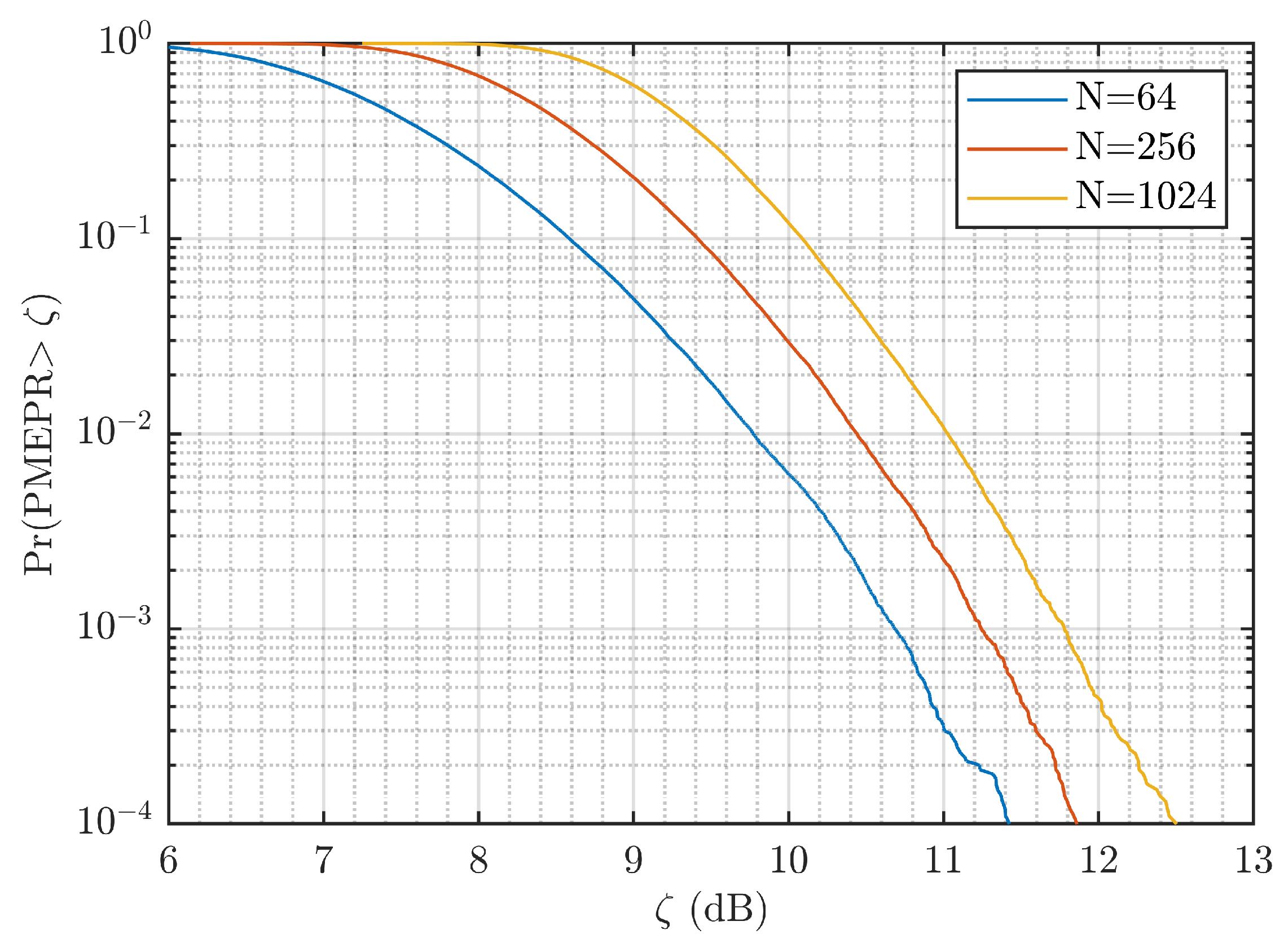
3.1. PMEPR
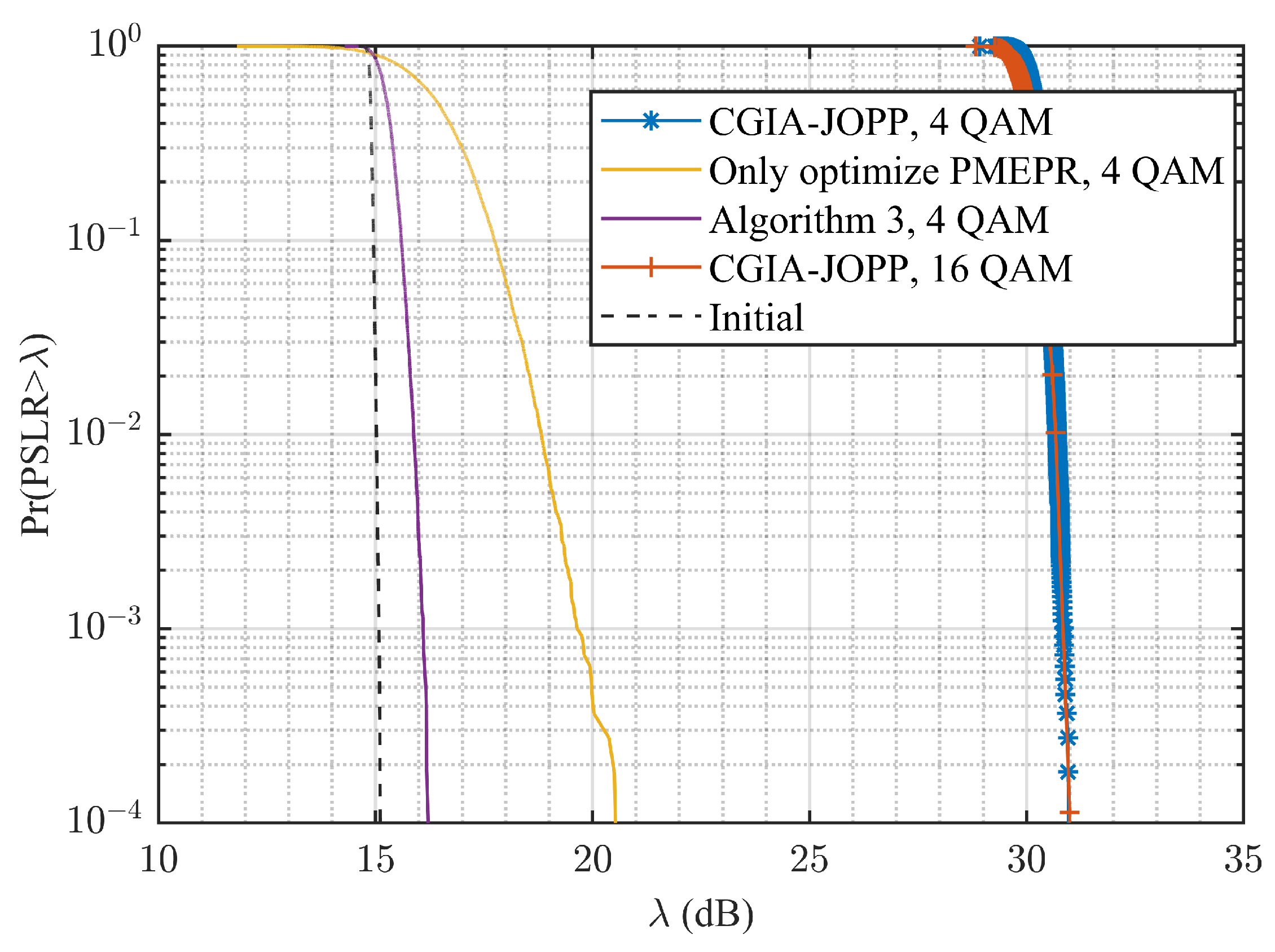
3.2. PSLR
3.3. Joint Optimization of PMEPR and PSLR
4. Proposed Algorithm and Its Complexity
4.1. Conjugate Gradient Analysis
4.2. Update Rules and Step Size
4.3. Descent Direction
4.4. Algorithm Summary and Complexity Analysis
| Algorithm 1: CGIA-JOPP |
1: Consider p, N, Q, , M. Store transmit data : , . Initialization conditions: , : , and . 2: 3: Compute step size according to Algorithm 2. 4: Update the reserved symbol vector: . 5: . 6: Compute the conjugate gradient according to (34). 7: Compute the descent direction according to (48). 8: . 9: a stopping condition is met, e.g., the sum of changes in the objective function value over 10 consecutive iterations does not exceed , then, transmit . |
| Algorithm 2: Compute step size |
1: Initialization conditions: , , , , ,. 2: 3: . 4: Update the step size: . 5: 6: . 8: if and is not met, let , and repeat Steps 4–7. 9: Compute according to (46). 10: . 11: a stopping condition is met, e.g., . |
5. Simulation Results
5.1. PMEPR and PSLR Performance of IRC Waveform
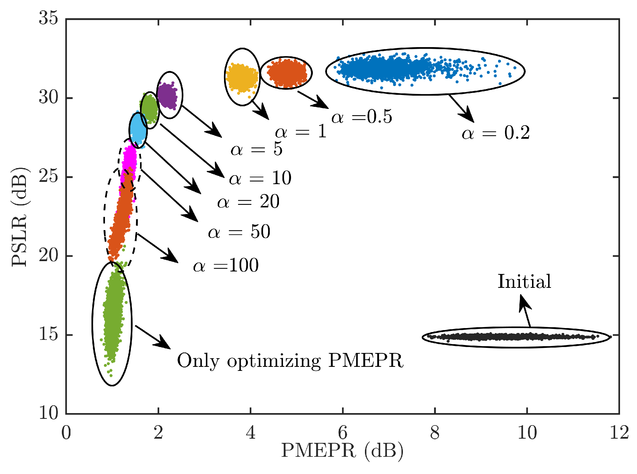
5.2. Tradeoff between PMEPR and PSLR
6. Discussion
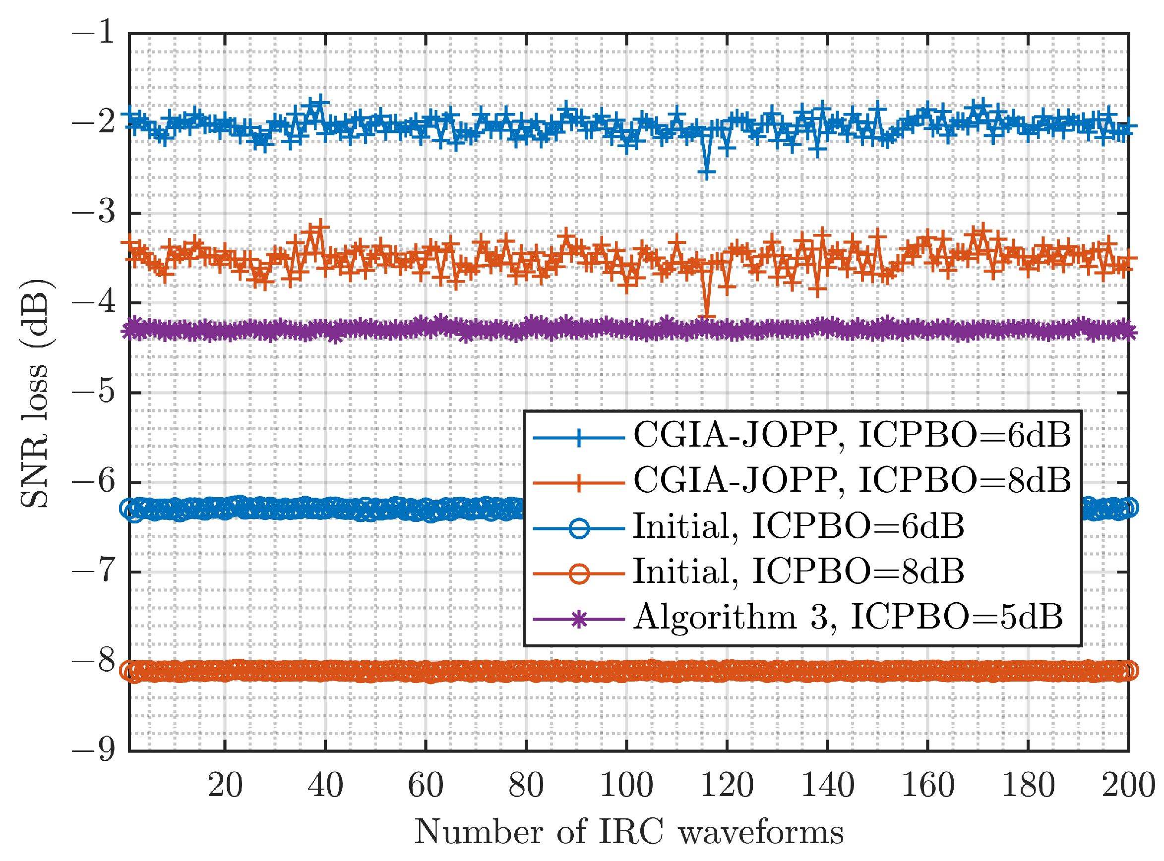
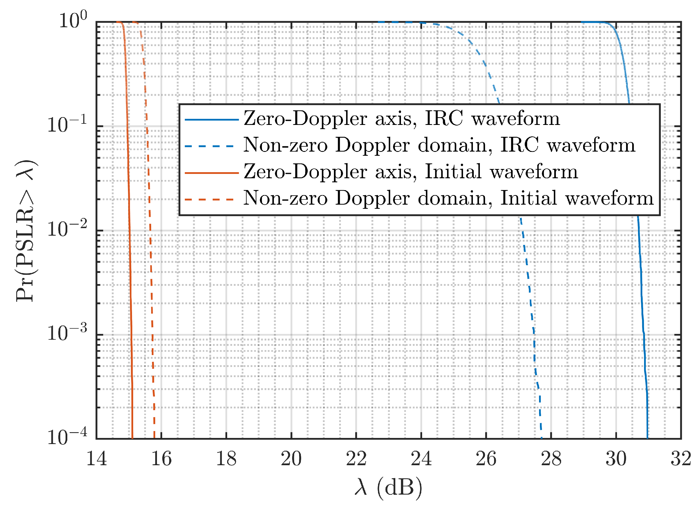
6.1. Radar Performance of IRC Waveform
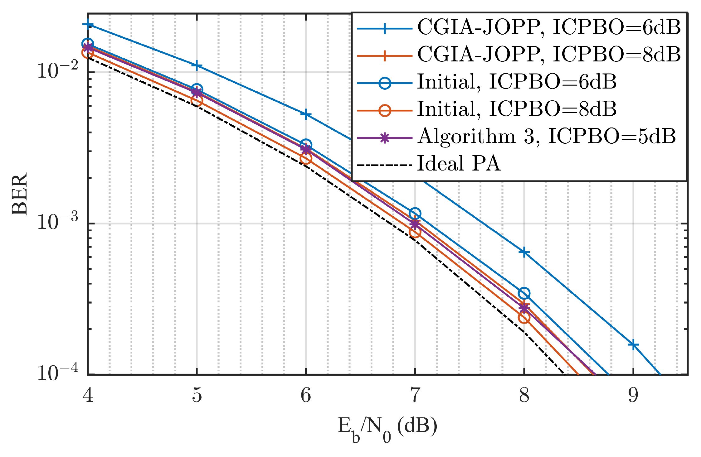
6.2. Communication Performance of IRC Waveform
7. Conclusions
Author Contributions
Funding
Institutional Review Board Statement
Informed Consent Statement
Data Availability Statement
Conflicts of Interest
References
- Frieden, R. The evolving 5G case study in spectrum management and industrial policy. Telecommun. Policy 2019, 43, 549–562. [Google Scholar] [CrossRef]
- Sturm, C.; Wiesbeck, W. Waveform design and signal processing aspects for fusion of wireless communications and radar sensing. Proc. IEEE 2011, 99, 1236–1259. [Google Scholar] [CrossRef]
- Dokhanchi, S.H.; Mysore, B.S.; Mishra, K.V.; Ottersten, B. A mmWave automotive joint radar-communications system. IEEE Trans. Aerosp. Electron. Syst. 2019, 55, 1241–1260. [Google Scholar] [CrossRef]
- Liu, F.; Masouros, C.; Ratnarajah, T.; Petropulu, A. On range sidelobe reduction for dual-functional radar-communication waveforms. IEEE Wirel. Commun. Lett. 2020, 9, 1572–1576. [Google Scholar] [CrossRef]
- Liu, Y.; Liao, G.; Xu, J.; Yang, Z.; Zhang, Y. Adaptive OFDM integrated radar and communications waveform design based on information theory. IEEE Commun. Lett. 2017, 21, 2174–2177. [Google Scholar] [CrossRef]
- Huang, Y.; Hu, S.; Ma, S.; Liu, Z.; Xiao, M. Designing low-PAPR waveform for OFDM-based radCom systems. IEEE Trans. Wirel. Commun. 2022, 21, 6979–6993. [Google Scholar] [CrossRef]
- Feng, Z.; Fang, Z.; Wei, Z.; Chen, X.; Quan, Z.; Ji, D. Joint radar and communication: A survey. China Commun. 2020, 17, 1–27. [Google Scholar] [CrossRef]
- Saddik, G.N.; Singh, R.S.; Brown, E.R. Ultra-wideband multifunctional communications/radar system. IEEE Trans. Microw. Theory Techn. 2007, 55, 1431–1437. [Google Scholar] [CrossRef]
- Blunt, S.D.; Yatham, P.; Stiles, J. BIntrapulse radar-embedded communications. IEEE Trans. Aerosp. Electron. Syst. 2010, 46, 1185–1200. [Google Scholar] [CrossRef]
- Rahmatallah, Y.; Mohan, S. Peak-to-average power ratio reduction in OFDM systems: A survey and taxonomy. IEEE Commun. Surv. Tutor. 2013, 15, 1567–1592. [Google Scholar] [CrossRef]
- Han, S.H.; Lee, J.H. An overview of peak-to-average power ratio reduction techniques for multicarrier transmission. IEEE Wirel. Commun. 2005, 12, 56–65. [Google Scholar] [CrossRef]
- Armstrong, J. Peak-to-average power reduction for OFDM by repeated clipping and frequency domain filtering. Electron. Lett. 2002, 38, 246–247. [Google Scholar] [CrossRef]
- Zhu, X.; Pan, W.; Li, H.; Tang, Y. Simplified approach to optimized iterative clipping and filtering for PAPR reduction of OFDM signal. IEEE Trans. Commun. 2013, 61, 1891–1901. [Google Scholar] [CrossRef]
- Rodrigues, M.; Wassell, I. IMD reduction with SLM and PTS to improve the error probability performance of nonlinearly distorted OFDM signals. IEEE Trans. Veh. Technol. 2006, 55, 537–548. [Google Scholar] [CrossRef]
- Huang, S.C.H.; Wu, H.C.; Chang, S.Y.; Liu, X. Novel sequence design for low-PMEPR and high-code-rate OFDM systems. IEEE Trans. Commun. 2010, 58, 405–410. [Google Scholar] [CrossRef]
- Mozeson, E.; Levanon, N. Multicarrier radar signals with low peak-to-mean envelope power ratio. IEE Proc.-Radar Sonar Navig. 2003, 150, 71–77. [Google Scholar] [CrossRef]
- Li, W.; Ren, P.; Xiang, Z. Waveform design for dual-function radar-communication system with golay block coding. IEEE Access 2019, 7, 184053–184062. [Google Scholar] [CrossRef]
- Jiao, Y.Z.; Liu, X.J.; Wang, X.A. A novel tone reservation scheme with fast convergence for PAPR reduction in OFDM systems. In Proceedings of the 2008 5th IEEE Consumer Communications and Networking Conference, Las Vegas, NV, USA, 10–12 January 2008. [Google Scholar]
- Tellado, J. Peak to Average Power Reduction for Multicarrier Modulation. Ph.D. Thesis, Stanford University, Stanford, CA, USA, 1999. [Google Scholar]
- Krongold, B.S.; Jones, D.L. An active-set approach for OFDM PAR reduction via tone reservation. IEEE Trans. Signal Process. 2004, 52, 495–509. [Google Scholar] [CrossRef]
- Hou, J.; Ge, J.; Gong, F. Tone reservation technique based on peak-windowing residual noise for PAPR reduction in OFDM systems. IEEE Trans. Veh. Technol. 2015, 64, 5373–5378. [Google Scholar] [CrossRef]
- Wang, L.; Tellambura, C. Analysis of clipping noise and tone reservation algorithms for peak reduction in OFDM systems. IEEE Trans. Veh. Technol. 2008, 57, 1675–1694. [Google Scholar] [CrossRef]
- Rong, J.; Liu, F.; Miao, Y. High-efficiency optimization algorithm of PMEPR for OFDM integrated radar and communication waveform based on conjugate gradient. Remote Sens. 2022, 14, 1715. [Google Scholar] [CrossRef]
- Sen, S. PAPR-constrained pareto-optimal waveform design for OFDM-STAP Radar. IEEE Trans. Geosci. Remote Sens. 2014, 52, 3658–3669. [Google Scholar] [CrossRef]
- Zhao, J.; Huo, K.; Li, X. A chaos-based phase-coded OFDM signal for joint radar-communication systems. In Proceedings of the 2014 12th International Conference on Signal Processing (ICSP), Hangzhou, China, 19–23 October 2014. [Google Scholar]
- Takase, H.; Shinriki, M. A dual-use system for radar and communication with complete complementary codes. In Proceedings of the 2014 15th International Radar Symposium (IRS), Gdansk, Poland, 16–18 June 2014. [Google Scholar]
- Hu, L.; Du, Z.; Xue, G. Radar-communication integration based on OFDM signal. In Proceedings of the 2014 IEEE International Conference on Signal Processing, Communications and Computing (ICSPCC), Guilin, China, 5–8 August 2014. [Google Scholar]
- Zuo, J.; Yang, R.; Luo, S.; Zhou, Y. Range sidelobe suppression for OFDM integrated radar and communication signal. J. Eng. 2019, 2019, 7624–7627. [Google Scholar] [CrossRef]
- Zuo, J.; Yang, R.; Cheng, W.; Li, X. Range sidelobe suppression of integrated radar and communication signals based on OFDM. J. Signal Process. 2020, 36, 1662–1667. [Google Scholar]
- Jiang, M.; Liao, G.; Yang, Z.; Liu, Y.; Chen, Y. Tunable filter design for integrated radar and communication waveforms. IEEE Commun. Lett. 2021, 25, 570–573. [Google Scholar] [CrossRef]
- Sebt, M.A.; Sheikhi, A.; Nayebi, M.M. Orthogonal frequency-division multiplexing radar signal design with optimised ambiguity function and low peak-to-average power ratio. IET Radar Sonar Navig. 2009, 3, 122–132. [Google Scholar] [CrossRef]
- Li, C.; Bao, W.; Xu, L.; Zhang, H.; Huang, Z. Radar communication integrated waveform design based on OFDM and circular shift sequence. Math. Probl. Eng. 2017, 2017, 9840172. [Google Scholar] [CrossRef]
- Wang, X.; Wu, Y.; Chouinard, J.-Y.; Wu, H.C. On the design and performance analysis of multisymbol encapsulated OFDM systems. IEEE Trans. Veh. Technol. 2006, 55, 990–1002. [Google Scholar] [CrossRef]
- Janaaththanan, S.; Kasparis, C.; Evans, B.G. A gradient based algorithm for PAPR reduction of OFDM using tone reservation technique. In Proceedings of the VTC Spring 2008-IEEE Vehicular Technology Conference, Marina Bay, Singapore, 11–14 May 2008. [Google Scholar]
- Zhang, X. Matrix Analysis and Applications; Tsinghua University Press: Beijing, China, 2004. [Google Scholar]
- Ding, L.; Geng, F. Principle of Radar, 3rd ed.; Xidian University Press: Xi’an, China, 2002. [Google Scholar]
- Jiang, T.; Guizani, M.; Chen, H.S.; Xiang, W.D.; Wu, Y.Y. Derivation of PAPR distribution for OFDM wireless systems based on extreme value theory. IEEE Trans. Wirel. Commun. 2008, 7, 1298–1305. [Google Scholar] [CrossRef]
- Liang, T.; Zhu, Y.; Fu, Q. Designing PAR-constrained periodic/aperiodic sequence via the gradient-based method. Signal Process. 2018, 147, 11–22. [Google Scholar]
- Polak, E.; Ribière, G. Note sur la convergence de directions conjugèes. Rev. Fr. Inform. Rech. Oper. 1969, 16, 35–43. [Google Scholar]
- Nee, R.V.; Prasad, R. OFDM for Wireless Multimedia Communications; Artech House: Boston, MA, USA, 2000. [Google Scholar]
- Zhang, X.; Ying, W.; Yang, P.; Sun, M. Parameter estimation of underwater impulsive noise with the class B model. IET Radar Sonar Navig. 2020, 14, 1055–1060. [Google Scholar] [CrossRef]
- Mahmood, A.; Chitre, M. Modeling colored impulsive noise by Markov chains and alpha-stable processes. In Proceedings of the OCEANS 2015, Genova, Italy, 18–21 May 2015. [Google Scholar]


| Parameter | Value |
|---|---|
| Baseband bandwidth | 128 MHz |
| Sampling frequency | 512 MHz |
| Number of subcarriers | 512 |
| Modulation | 4 QAM/16 QAM |
| Single OFDM symbol duration | 4 μs |
| Cyclic prefix duration | 10 μs |
| Number of OFDM symbols | 3 |
| Pulse width | 22 μs |
| Tone reservation ratio | |
| p in -norm | 10 |
Publisher’s Note: MDPI stays neutral with regard to jurisdictional claims in published maps and institutional affiliations. |
© 2022 by the authors. Licensee MDPI, Basel, Switzerland. This article is an open access article distributed under the terms and conditions of the Creative Commons Attribution (CC BY) license (https://creativecommons.org/licenses/by/4.0/).
Share and Cite
Rong, J.; Liu, F.; Miao, Y. Integrated Radar and Communications Waveform Design Based on Multi-Symbol OFDM. Remote Sens. 2022, 14, 4705. https://doi.org/10.3390/rs14194705
Rong J, Liu F, Miao Y. Integrated Radar and Communications Waveform Design Based on Multi-Symbol OFDM. Remote Sensing. 2022; 14(19):4705. https://doi.org/10.3390/rs14194705
Chicago/Turabian StyleRong, Juan, Feifeng Liu, and Yingjie Miao. 2022. "Integrated Radar and Communications Waveform Design Based on Multi-Symbol OFDM" Remote Sensing 14, no. 19: 4705. https://doi.org/10.3390/rs14194705
APA StyleRong, J., Liu, F., & Miao, Y. (2022). Integrated Radar and Communications Waveform Design Based on Multi-Symbol OFDM. Remote Sensing, 14(19), 4705. https://doi.org/10.3390/rs14194705