Abstract
An enhanced filter for floating Doppler wind lidar motion correction is presented. The filter relies on an unscented Kalman filter prototype for floating-lidar motion correction without access to the internal line-of-sight measurements of the lidar. In the present work, we implement a new architecture based on two cooperative estimation filters and study the impact of different wind and initial scan phase models on the filter performance in the coastal environment of Barcelona. Two model combinations are considered: (i) a basic random walk model for both the wind turbulence and the initial scan phase and (ii) an auto-regressive model for wind turbulence along with a uniform circular motion model for the scan phase. The filter motion-correction performance using each of the above models was evaluated with reference to a fixed lidar in different wind and motion scenarios (low- and high-frequency turbulence cases) recorded during a 25-day campaign at “Pont del Petroli”, Barcelona, by clustered statistical analysis. The auto-regressive wind model and the uniform circular motion phase model permitted the filter to overcome divergence in all wind and motion scenarios. The statistical indicators comparing both instruments showed overall improvement. The mean deviation increased from 1.62% (without motion correction) to −0.07% (with motion correction), while the root-mean-square error decreased from 1.87% to 0.58%, and the determination coefficient () improved from 0.90 to 0.96.
1. Introduction
In the context of onshore wind energy, meteorological masts (metmasts) are the traditional instrument used for the assessment of future wind farms’ locations, as well as wind monitoring for wind-turbine operation purposes. However, in the case of offshore wind farms, as they are installed farther offshore and into deeper water regions, the deployment of metmasts planted on the seabed may be too expensive or even not feasible [1,2]. Offshore wind energy is one of the most expensive sources of energy, having the second highest levelized cost of energy (LCOE, 2020) after concentrating solar power, with LCOE values of 0.084 USD/kWh and 0.108 USD/kWh, respectively [3,4]. Therefore, there is a need for cost reduction in the wind energy industry. In recent decades, Doppler wind lidars (DWLs) have proved themselves as a cost-effective solution and have been considered as a replacement for costlier metmasts [5,6]. When placed over floating platforms or buoys, DWLs are able to assess the offshore atmosphere in a flexible way, since they can be re-deployed at multiple locations and cover large areas [5].
The floating DWLs’ (FDWLs) main goal is to accurately assess the wind resource at specific (usually remote) offshore locations in order to study the viability of future offshore wind farm projects. Towards this purpose, they need to integrate in the same device an energy generating system, a data-logging system, a communications system, and a lidar motional attitude measurement system along with the DWL [7]. These needs were satisfied according to the wind industry requirements, following a roadmap for the commercial acceptance of floating LIDAR technology [8], and guides for the best practices for their application [9].
Nowadays, FDWLs are accepted in the wind energy industry as the de-facto instrument for offshore wind resource assessment, reaching a commercial stage [8]. Multiple measurement campaigns have demonstrated their capability to measure in a robust way the mean horizontal wind speed () and wind direction () after yaw correction, at a 10-min level [10,11,12,13,14]. Recently, FDWLs have been used to measure incoming wind fields before contacting wind turbines in order to reduce loads and oscillations on their blades. Particularly, they are being considered for assisted stabilization control systems of floating wind turbine generators [15]. This requires an accurate track of the instantaneous wind vector by FDWLs. However, waves induce 6-degree-of-freedom (DoF) motion on the FDWL. FDWL motion affects DWL measurements [16], inducing an error in the lidar-retrieved wind vector and adding variance to the lidar measurements in comparison to fixed lidars. Therefore, it is essential to estimate the motion-free true wind vector, i.e., to take wave-induced motion out of the raw (motion-corrupted) measured wind. This is often called deconvolution and is usually carried out by means of adaptive filters such as the Kalman filter.
When measuring wind turbulence intensity (), FDWLs measure higher due to the wave-induced variance addition [14,17]. , defined as the ratio of the standard deviation to the mean , is one of the most relevant parameters to be measured in wind energy due to its relevance on wind turbine operation and power production [18,19]. For instance, wind turbine models need to predict power production in varying atmosphere environments [20]. Moreover, erroneous values in the site assessment phase may result in over-designed wind turbines, which would increase the wind farm project cost [21].
Multiple studies have so far addressed the impact and correction of motion-induced measurement errors using floating lidars [14,16,21,22,23,24,25,26,27,28,29]. Thus, the works of Wolken-Möhlmann et al. [22] and Gottschall et al. [27] are representative of the first studies on the simulation and offshore tests of lidars on floating platforms. Schlipf et al. [29] demonstrated the potentialities of theoretically modeling a lidar system in order to reconstruct the wind field from corrupted lidar measurements. Regarding the ZephIR lidar, Pitter et al. [23] studied its performance when mounted on buoys or wind turbines and proved that the 10-min averaged wind speed recorded by ZephIRs is very resilient to motion. It was also found that angular motion is the main error source. The study of Bischoff et al. [26] addressed the motion compensation of FDWLs by means of a wind field reconstruction method and demonstrated that the quality of horizontal wind measurements can be improved if the lidar attitude is known. Tiana-Alsina et al. [16] presented a mechanical approach by deploying the ZephIR-300 lidar on a cardanic frame. This method was able to compensate for most of the rotational motion but not for the translational one. However, mechanical resonance was a risk to be minimized and the cardarnic method increased the hardware costs of the instrument.
More recently, Gutiérrez-Antuñano et al. [24] presented an adaptive averaging window technique to filter out the motion-induced errors on measurements. The window length has to be comparable to the tilting period of the lidar (roll and pitch motion only). Unfortunately, this method requires the lidar wind-vector sampling frequency to be higher (approximately by a factor 2) than the wave motion frequency, which is not always the case. In 2020, Kelberlau et al. [21] proposed a signal processing approach, in which the 6-DoF motion of the FDWL were taken into account to correct for the motion-induced error at a Line-of-Sight (LoS) level. The algorithm demonstrated itself able to take the motion out in multiple wind and sea scenarios in a coastal environment but it requires access to the high-frequency internal LoS measurements of the lidar. The latter is usually undisclosed information for most commercial continuous-wave lidars.
Recently, an FDWL motion-correction method for a focusable continuous-wave lidar based on the unscented Kalman filter (UKF) was presented in [25]. Without having access to the lidar internal LoS measurements, the UKF recursively estimates on the run the motion-corrected wind vector by considering the lidar 6 DoF motion and emulating the FDWL measurement process. The method demonstrated to be able to correct FDWL measurements for motion-induced additive . Thus, when comparing the FDWL to a reference fixed lidar, the apparent was reduced from −1.70% (without correction) to 0.29% (with correction). However, moderate differences between the two lidars remained, which manifested with a coefficient of determination of 0.93. Moreover, this first UKF prototype overcompensates the , which we hypothesize is caused by the assumptions of oversimplified random process models of the random walk (RW) type for both the wind and initial scan phase. The flaws of these models demonstrate prominently in high wind turbulence or transitioning scenarios, which may often cause filter divergence [30]. Therefore, it is sensible to assume that refined wind and lidar initial scan phase models are to enhance filter tracking and reduce divergence.
In the present work, we study the impact of different wind and phase model combinations on the motion-correction capabilities of the filter as well as the impact of different near-shore sea and atmospheric scenarios on the filter performance. The novelty of the enhanced filter lies in the expected superior wind-tracking capabilities of the filter, particularly in high-frequency turbulence regimes and in the operation of the filter without having access to the lidar internal LoS measurements.
This paper is structured as follows: In Section 2, Section 2.1 presents the “Pont del Petroli’’ near-shore experimental campaign, and Section 2.2 reviews motion correction using the UKF [25], presents the enhanced wind and scan initial-phase models and formulates the new motion-correction filter using two cooperative filters (the so-called “dual UKF’’). Next, Section 3 discusses the motion-compensation performance of the new filter in two different case examples and evaluates global statistics for the whole campaign. Eventually, Section 4 gives concluding remarks.
2. Materials and Methods
Next, in Section 2.1, the instruments and experimental set-up at “Pont del Petroli’’ are presented. In Section 2.2, the motion-correction UKF is reviewed and different wind and initial scan phase models are explored and compared. Eventually, the enhanced motion-correction UKF using two cooperative filters is formulated.
2.1. Materials
NEPTUNE proof-of-concept buoy. The floating lidar system was especially conceived for offshore wind measurements. The lidar was mounted on a cardanic frame, intended for mechanical motion compensation. Apart from the lidar, this proof-of-concept buoy hosted two inertial measurement units (IMUs) to measure the lidar and buoy motion. The first IMU, the “lidar IMU’’, was mounted on the cardanic frame, and the second one, the “buoy IMU’’, was mounted on the buoy’s bottom. These IMUs measured the six DoF motion (i.e., roll, pitch, yaw, surge, sway and heave) of both the lidar and the buoy at a 10 Hz sampling frequency. The 50-Hz line-of-sight attitude data was interpolated using the 10-Hz IMU data. According to the Nyquist sampling theorem [31], the sampling frequency of the IMUs must be greater than twice the motion’s highest frequency in order to perfectly recover the original analog motion signal from the discrete values produced by sampling. Assuming wave periods longer than 2 s (i.e., wave frequencies smaller or equal than 0.5 Hz), the 10 Hz IMU sampling frequency exceeds the Nyquist wave frequency limit (1 Hz) by a factor 10.
ZephIR 300 lidar. ZephIR 300 is a focusable continuous-wave DWL. The lidar uses a rotating prism to deflect the emitted laser beam (Figure 1) and create a scanning cone of 30-degree width from the zenith. The prism rotates with uniform circular motion at a rate of one rotation per second (360 degs/s). The lidar uses the velocity–azimuth display (VAD) algorithm [32] to retrieve the wind vector from the 50 line-of-sight (LoS) velocity measurements in a scan (i.e., at a rate of 50 samples/s). By refocusing, the lidar is able to sequentially measure at a set of user-defined heights. However, this is performed at the expense of reducing the sounding time resolution at a given height by a factor greater than the number of sounding heights, because dead times are needed to refocus from one height to another. When the lidar measures at a single height (no refocusing) the wind vector is retrieved with a nearly uniform resolution of 1 s (1 scan/s). This was the preferred option in this study, and a fixed height of 100 m was used. The ZephIR 300 also provides a series of internal parameters for data-quality control. These parameters include rain flags, backscattering and spatial variation (), among others. indicates the quality of the VAD fitting, which is a proxy of the spatial uniformity of the wind field during the lidar scan, which, in turn, is directly related to the [24]).
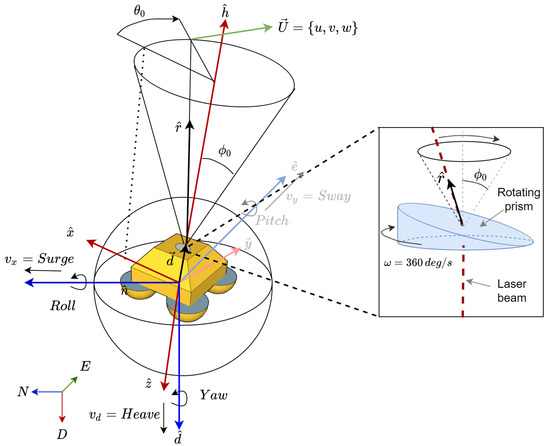
Figure 1.
Geometry of the NEPTUNE FDWL proof-of-concept buoy. Inset shows the lidar rotating prism used for deflection of the laser beam.
Dataset. Specifically, the dataset comprised (i) wind measurements from the reference fixed DWL sited at PdP pier, (ii) wind measurements from the FDWL, (iii) fixed DWL and FDWL buoy internal parameters for data-quality control and (iv) 6 DoF motion measurements obtained by the “lidar IMU’’ and the “buoy IMU’’. HWS values were measured by the fixed reference lidar and ranged from 1.2 to 14.4 m/s, whereas values ranged from 0.90% to 24.89%. According to the manufacturer’s specifications [23], lidar measurement records lower than 2 m/s were considered unreliable; therefore, records with 10 min mean lower than 2 m/s were filtered out.
2.2. Methods
Recently, the authors presented a robust adaptive UKF for FDWL motion compensation [25]. The filter takes advantage of the knowledge of the floating lidar buoy dynamics and the VAD algorithm to estimate the sought-after motion-corrected wind vector.
2.2.1. Motion-Correction UKF Review
The UKF estimates the hidden state vector (), which is formed by the “true’’ wind vector (), i.e., motion-free, and the lidar initial scan phase () (hereafter, the “initial phase’’) given by the measurement vector (), which is the lidar-measured motion-corrupted wind vector. The state vector is formulated as follows:
where is the wind vector defined by the , and vertical wind speed () components at discrete time (sampling period, s):
The FDWL measurement vector is written as follows:
where , and are the motion-corrupted , and measured by the FDWL at time .
The filter relies on two steps to estimate the state vector, the prediction step and the innovation step.
The prediction step is defined by the following set of equations:
where sub-indexes denote the estimate at step n based on information up to step m.
Equation (4) is the prediction equation in which the predicted or “future’’ state vector () is related to the previous estimate () by means of a state-transition function . Function merges the wind and initial-phase RW models, and , respectively, into a single body. is the so-called process-noise vector or state-vector “driving’’ noise, which is assumed to be a zero-mean Gaussian with covariance . In plain words, is the “random jump step’’ used by both the wind and initial phase RW models. In a state-space representation [30] (see Section 2.2.5), functions and both are identity matrix , and the prediction equation takes the following form:
On the other hand, Equation (5) is the measurement equation, which relates the predicted state vector () to the predicted measurement vector () through measurement function and measurement noise . The measurement function takes as input and matrix . denotes the 50 × 6-dimension block-vector describing the 6-DoF motion for each of the 50 LoS measurements in a lidar scan. The IMU-measured motion time series at 10 Hz sampling rate is interpolated to 50 Hz in order to match the LoS measurements. Function simulates the FDWL motion-corrupted wind vector (). is defined as the function composition (so-called chain calculus):
where is the function modeling the rotational motion influence on each of the 50 LoSs of the lidar conical scan. The inputs to are the IMU-measured lidar rotation attitude (roll, pitch and yaw) at each LoS and sampling time during the conical scan (50 LoS/scan, equivalently, 50 Hz sampling rate) and the initial phase, . The output is the set of estimated motion-corrupted lidar pointing directions denoted as , in the global North–East–Down (NED) frame of reference.
Similarly, is the function modeling the translational motion influence on the LoSs. The inputs are the IMU-measured lidar translational velocity (surge, sway and heave) at discrete time , the predicted (i.e., motion-compensated) state-vector wind, , and the set of motion-corrupted LoSs (, ) computed from the above-mentioned . The function output is the set of the 50 motion-corrupted velocity measurements along the respective LoSs (, ) during the DWL scan.
Conceptually, composite function describing the motion model is also of application to floating wind turbine generators, as it can be embedded in the design of closed-loop stabilization systems [33,34,35].
Finally, function takes these 50 motion-corrupted LoS velocities () and computes motion-corrupted wind vector by means of the VAD algorithm.
The innovation step is the step at which the filter corrects the a priori estimation of state vector with the actual measurement information at time :
where is the FDWL wind-vector measurement, and is the Kalman gain. The latter relates the measurement prediction error, , to the state-vector prediction error, , as .
Estimation of noise-covariance matrices. At each recursive step, the UKF estimates the process-noise and measurement-noise covariance matrices ( and , respectively, where E is the expectancy operator). The covariance matrices are adaptively updated via forgetting factors and :
Refer to Appendix A for details.
2.2.2. Enhanced Wind Models: The Auto-Regressive Approach
In this section, we aim to revisit the basic RW wind model of Equation (6) for the improved estimation of the wind process spectrum by the UKF. To this end, different models are presented and compared in terms of their power spectral density (PSD) with reference to the fixed lidar. The PSD indicates the signal power distribution as a function of the frequency [36].
Random walk (Equation (6)) models the state-vector wind component, (Equation (1)), at discrete time as the superposition of the measured wind vector, , at previous time plus a stochastic term :
Alternatively, we propose a low computationally demanding, straightforward wind model based on an auto-regressive (AR) process of order P, AR(P). In this model, the measured wind vector, , at each time is a linear combination of its P previous values (i.e., at time instants ) plus a stochastic term modeling an imperfectly predictable term. The AR(P) model is formulated as follows:
where is the -dimension wind vector at time (Equation (2)); , and are the -dimension vectors denoting the measured
, and at previous times . is zero-mean white noise with constant variance . , , , are the -dimension vectors containing the AR(P) model coefficients for the , and wind components, respectively:
The AR-process PSD is computed by means of the Yule–Walker equations [36].
The accuracy of the AR wind model depends on the process order as discussed next:
Thus, in Figure 2, we compared the PSD of four different 10 min time series measured by the fixed lidar with the estimated PSDs using different random process models. Two high- and two low-frequency wind scenarios (panels (a,b) and (c,d), respectively) characterized by low and high s ((a,c) and (b,d), respectively) were chosen. It can be observed that the RW model was not able to follow all the spectral details of the measured PSD in high frequency scenarios. At low frequencies ( Hz), RW was biased up to 4 dBs. In addition, RW was not able to follow the second lobe of the lidar-measured PSDs at Hz. On the other hand, the RW matched quite well the reference PSD in low frequency scenarios irrespective of the chosen. Regarding the AR models, they emulated more accurately the PSD in high frequency scenarios in comparison to the RW model. Moreover, it is evident that the higher the process order was, the better the model capability to equal the measured PSD was. The AR process order P was determined on the basis of the lowest order, ensuring a difference lower than 3 dB between the secondary lobes of the measured and emulated PSDs in high-frequency scenarios (Figure 2a,b). By experiment, the AR process order was found.
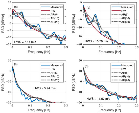
Figure 2.
Comparison between the PSD measured by the fixed lidar (PdP campaign; Barcelona; 10 min time series) and the PSDs estimated from a set of different RW and AR random process models (see legend). Panels (a,b): high-frequency wind scenarios (19 June 2013, 17:10 LT; and 28 June 2013, 12:40 LT, respectively). Panels (c,d): low-frequency wind scenarios (24 June 2013, 12:30 LT, and 22 June 2013, 12:10 LT, respectively).
2.2.3. Lidar-Scan Initial-Phase Model
The UKF lidar motion-correction algorithm by Salcedo-Bosch et al. [25] assumes the oversimplification that initial phase is a random variable with uniform distribution over 0-360 deg, and that there are independent phases from one conical scan to the next [14]. An RW model was considered for the initial phase:
where and are the initial phases at discrete times and , respectively, and is a random variable with uniform distribution over deg.
Alternatively, here, we propose a phase model based on the kinematics of the DWL rotating prism used to implement the scanning mechanism (Section 2.1 and Figure 1, inset) that breaks this independence assumption. Because the prism has uniform circular motion (UCM) at a rate of 360 deg/s, if the initial phase is known at a given time instant, it can be known elsewhere in time. The UCM initial-phase model can be formulated as follows:
where and are the initial phases (in degrees) at discrete times and , respectively, and is the time lag between and . Experimentally, there is a small time lapse between consecutive lidar scans as well as a variability in this time lapse, which can be caused by CPU internal processes or the re-focusing of the lidar at different heights. This leads to observed initial phases, , with apparent uniform distribution between 0 and 360 deg.
Figure 3 shows the initial-phase time series, , for the UCM model in response to the time-lag series, . The resulting initial-phase distribution is also shown. The time-lag series was generated from one hour of lidar-recorded timestamps. The initial phase at start time s was = 180 deg. In Figure 3b, it can be observed that the time lag, , usually departed from the nominal ≃1 s scan time (baseline), with noticeable lag dropouts approximately every 15 s being caused by the lidar internal CPU interruptions. The initial-phase time series shown in Figure 3a tentatively demonstrated uniform random behavior over [0, 360) degs. The uniform distribution was corroborated in the 30 deg bin histogram in Figure 3c.
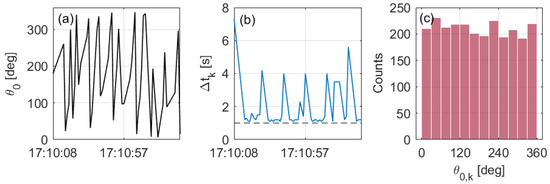
Figure 3.
The UCM initial-phase model (19 June 2013; 17:10–17:20 LT; PdP campaign). (a) Initial-phase time series, (sub-segment 17:10:08–17:11:35 LT). (b) Time-lag time series, . Baseline (dashed line) indicates the 1 s nominal lidar scan time. (c) Histogram plot of the initial phase (panel (a)).
2.2.4. Dual UKF Estimation
We propose a dual UKF approach consisting of two unscented Kalman filters working cooperatively: the main filter (UKF1), which estimates the wind vector (Equation (12)) and initial phase, and the auxiliary filter (UKF2), which estimates the weight vector (Equation (13)). The motivation behind this is the non-stationarity of wind fields. Although, in theory, the wind process is usually considered stationary over short-term intervals (≃15 min [37]), in practice, it is non-stationary and is dependent on the atmospheric conditions. Therefore, weight vector , which describes the AR model coefficients, is an unknown set of random variables that needs to be continuously estimated at each discrete time along with state vector .
As illustrated in Figure 4, the weight vector estimated at time by UKF2, , is used by UKF1 to estimate the wind vector at the prediction step. Similarly, the wind-vector and initial-phase estimates at , denoted as and , respectively, which are part of the state-vector estimated by UKF1, are used to estimate the weight vector at the UKF2 innovation step. Both filters use the motion-corrupted wind vectors retrieved by the FDWL () at both the prediction and innovation steps, and the IMU-measured FDWL attitude (6 DoFs) at the prediction step. The formulation of the two filters is detailed in the subsections below.
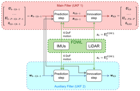
Figure 4.
The dual UKF approach. (Red box) Main filter (UKF1) used to estimate the motion-free wind vector (, i.e., the “true’’ wind vector at time ) and initial phase . (Blue box) Auxiliary filter (UKF2) used to estimate the weight vector defining the AR wind model. (Green Box) FDWL block. Green arrows depict that both filters assimilate FDWL 6 DoF motion information from the buoy IMUs as well as the motion-corrupted FDWL wind retrievals, . The black arrows depict the exchange of information between filters UKF1 and UKF2.
2.2.5. Main UKF
The main filter, UKF1, exhibits great similarities with the former motion-correction filter designed by Salcedo-Bosch et al. [25] (refer to Section 2.2.1). Similar to such implementation, UKF1 aims to estimate the wind vector and initial phase from motion-corrupted wind data; however, this is achieved using enhanced models in the version here shown. Thus, UKF1 uses the AR(P) model instead of RW for the wind process and the UCM model instead of RW for the initial phase.
In order to formulate UKF1, the previous equation for the state vector (Equation (1)) is reformulated by including the P past wind-vector estimations relative to times from to :
The state-transition function of the main filter, , is composed of AR wind-model state-transition function and UCM initial-phase state-transition function :
where is the current “a posteriori’’ estimate of the weight vector by UKF2, and and are written in state-space formulation upon the models of Equation (13) and Equation (15), respectively. Explicitly:
and:
In Equations (18) and (19) above, the state-space formulation provides a convenient way to rewrite the simple random process description of Equations (13) and (15) into the vector forms of Equations (18) and (19), respectively. The advantage of this state-space representation is that it allows the AR wind model and UCM initial-phase model to be easily integrated into filter Equation (4) through state-transition function .
Measurement vector and measurement function are identical to the UKF filter described in Section 2.2.1 with measurement function defined by Equation (7).
2.2.6. Auxiliary UKF
The auxiliary filter, UKF2, aims to estimate AR wind-model weight vector . Therefore, the state-vector is vector to be estimated, formed by the , and as AR process coefficients of P-th order:
Because it is assumed that random step changes in any of the weights occur with equal probability and are independent of each other, the state-transition model is considered as random walk [38]. It is formulated as follows:
Similar to UKF1, the UKF2 observation vector is FDWL-measured wind vector . In expanded form:
where , and are the FDWL-measured (i.e., motion-corrupted) , and , respectively.
The UKF2 measurement function, , relates the “a priori’’ estimation of weight vector to the motion-corrupted measurement vector . To perform the above, the P previous motion-corrected wind vectors estimated by UKF1 () must be propagated to the AR wind model via function ) and weights in order to predict motion-corrected or “true’’ wind vector at present time . Then, the predicted wind vector is transformed by UKF1 lidar measurement function to predict measured motion-corrupted wind vector in the recursive loop of the filter. These steps can be written as follows:
Note that, for short, in Equation (7), Section 2.2.1.
Concerning filter initialization, both the main and auxiliary filters use a rough estimate of the motion-corrected wind-vector time series computed using the window averaging technique [24]. The initial weight vector, , is derived by fitting an AR model to the rough motion-corrected time series. The process-noise covariance initial matrices are derived as the mean squared error between the observations and the predictions by the fitted AR model. Measurement-noise covariance matrices are initialized from the rough motion-corrected time series as in [25].
2.2.7. Model Intercomparison Methodology
In order to assess the motion-correction performance of the improved wind and initial-phase models presented in Section 2.2.2 and Section 2.2.3, two model combinations were considered (Table 1):

Table 1.
Basic and enhanced model combinations studied to assess the motion-correction filter performance.
- (1) Basic model: Both the wind process and initial phase are modeled as RWs;
- (2) Enhanced model: The wind process is modeled as an AR process (order ) and the initial phase as UCM (see Section 2.2.3).
For each of the model combinations above, the motion-correction performance was analyzed in terms of and its mean deviation with reference to the fixed lidar. The statistical descriptors below were considered.
(a) Floating-lidar measurements with and without correction ( and , respectively) were compared against fixed-DWL measurements (), which were used as reference. Model comparisons were carried out considering different motion scenarios clustered as a function of (i) mean WD, (ii) mean HWS and (iii) FDWL mean tilt. The mean tilt was computed from 10 min roll and pitch-tilt measurements [39]:
where is the number of samples in a 10 min interval, and ms is the IMU sampling time increment (10 Hz sampling frequency).
(b) The mean deviation (MD) of the FDWL motion-corrected with reference to the fixed lidar was computed as follows:
where N is the number of measurements in each cluster.
3. Results and Discussion
In this section, the performance of the enhanced motion-correction UKF is studied. First, two case examples are presented under low- and high-frequency turbulent regimes. Second, the performance of the basic and enhanced filters in terms of estimation is compared under different motion and wind scenarios. Third, the motion-correction accuracy achieved by both filters is examined through numerical analysis. Finally, the limitations of the enhanced filter are presented and discussed.
3.1. Case Examples
Two case examples are presented next to illustrate the comparative performance between the basic and enhanced models of Section 2.2.2 and Section 2.2.3, respectively, under two different turbulent regimes: (i) low-frequency turbulence (Figure 5) and (ii) high-frequency turbulence (Figure 6). These figures compare the 10 min motion-corrected time series and related spectra when using the basic and enhanced models with reference to the fixed lidar and the uncorrected FDWL. The error bars depicted are indicative of the uncertainty in the estimations. The uncertainty is computed as the square root of the main diagonal first element of the a posteriori error covariance matrix (Algorithm A1, step 3 in Appendix A). The main diagonal is the a posteriori state-noise error variance vector associated with the state vector (see Equation (1)), so that its first element (Equation (2)) corresponds to the error [40]. A similar approach was followed by Araújo et al. [41] to assess the Kalman filter error on the estimation of the atmospheric boundary layer height.
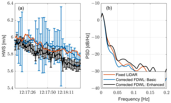
Figure 5.
Case example #1: Low-frequency turbulence scenario (PdP campaign; 22 June 2013; 12:10 LT). time-series measured during PdP campaign by the fixed lidar and the FDWL with motion correction considering the basic and enhanced models combinations. (a) Time-series comparison between the basic and enhanced floating-lidar motion-correction models with reference to the fixed lidar. (b) Related PSDs.
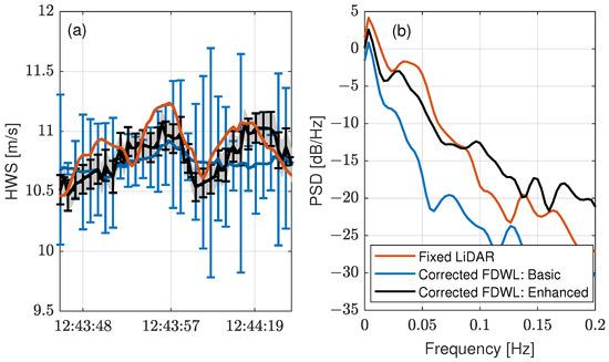
Figure 6.
Case example #2: High-frequency turbulence scenario (PdP; 28 June 2013; 12:40 LT). Same legend as in Figure 5. Note the larger Y-axis limits in panel (a) to accommodate much higher variations.(b) Related PSDs.
The first case is shown in Figure 5. The weak turbulence of the wind in Figure 5a was evidenced by the fixed-lidar time series, showing an approximately constant ( ≈ 6 m/s) along with slow speed variations (notice that the Y-axis scale only spans 1.5 m/s). In the PSD plot of Figure 5b, the prominent low-frequency behavior of the turbulence was associated with a primary-to-secondary lobe level (PSLL) as high as 29 dB. The primary lobe, which concentrates most of the wind energy, was close to 0 Hz and peaked at 4 dBs, while the secondary lobe, which assimilates rapid turbulent variations, lay at 0.08 Hz and peaked at −25 dBs.
In Figure 5a, both the basic and the enhanced model combinations enabled the filter to motion-correct the corrupted FDWL measurements and to acceptably track the fixed-lidar reference. This is re-encountered in Figure 5b, with similar spectra between the enhanced and the basic models, albeit with the remark that the enhanced models overestimated the high-frequency components above 0.1 Hz. Moreover, both model combinations were able to correctly estimate the true wind (figure not shown) as = 2.77% (basic) and 2.87% (enhanced), which were nearly identical to the reference , = 2.76%.
However, the error bars evidence that estimates from the basic filter have very high uncertainties as compared to the enhanced filter. This is due to the improved wind and initial phase models used, providing more accurate a priori estimation of the wind vector.
The second case is shown in Figure 6. In Figure 6a, the reference time series measured by the fixed lidar demonstrated rapid and more intense variations, including sudden wind gusts lasting between 20 and 30 s. These fast variations manifested in the PSD of Figure 6b as a much lower PSLL than that in Figure 5b. The PSLL was only 7 dB (the main lobe around 0 Hz (low frequencies) was at ≃4 dB, and the secondary lobe at ≃−3 dB lay between 0.03 and 0.05 Hz (high frequencies)).
From the temporal series plots, it arises that the motion-correction filter was not able to follow the peaks when using the basic model combination. These peaks were treated by the filter as if they were noise; therefore, such turbulent situations led to biased estimations. In contrast, the enhanced combination permitted the filter to track the wind gusts. Based on the error bars shown in Figure 5 and Figure 6, it emerges that in a fast-changing wind scenario, the enhanced-filter uncertainties in the estimates remain small and attain similar values to those attributable to low-frequency scenarios. The PSD demonstrated that the basic model combination (blue trace) underestimated all frequency components higher than approximately 0.02 Hz by about ≃8 dB (blue trace versus black trace). On the contrary, the enhanced combination permitted the filter to reasonably follow the high-frequency wind components up to 0.1 Hz. The numerical estimation yielded = 1.17% (basic), and 2.08% (enhanced) as compared with = 2.07%. It is important to highlight that higher AR-model orders (for example, and ) yielded biased estimations of both the PSD and due to the much longer convergence time required by the filter. Therefore, in a fast-changing wind scenario, such as the one in Figure 6, the filter may not be able to converge.
3.2. Global Statistics
To complete the analysis, the performance of the motion-correction model combinations mentioned above (Section 2.2.7) was studied by comparing the 10 min measured by the FDWL (before and after motion correction) with reference to the fixed lidar under different wind and motion conditions. In total, 1786 data records (from 6 to 30 June 2013) from the PdP experimental campaign were used. The statistical database was filtered out for outliers according to the quality assurance criteria described in detail in [25]. In brief, the removed outliers encompassed rain-flagged data, measurement values outside the 1–80 m/s range, values higher than 0.2 and backscattering coefficients smaller than 0.02.
The 10-min mean and measured by the FDWL without motion compensation matched almost ideally the measurements of the reference fixed lidar as expected from previous studies [11,21,24,42]. Regarding the mean , when regressing FDWL data onto fixed-lidar for the whole campaign, the coefficient of the determination () was 0.997, linear regression (LR) slope was 0.99 and LR offset was 0.06 m/s. Regarding the mean , the coefficient of determination was , LR slope 0.98 and LR offset 0.41 deg. These values are compliant with the key performance indicators defined by the Carbon Trust Offshore Wind Accelerator [8]. The same indicators were obtained after motion correction with both the basic and the enhanced filters.
Figure 7 shows the performance of the motion-correction model combinations mentioned above in Section 2.2.7, studied by comparing the measured by the fixed lidar and by the FDWL (before and after motion correction) under different wind and motion conditions. The input statistical variables of the study or clustering variables were , and buoy tilt angle, and the output ones were mean , and FDWL translational velocity.
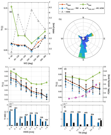
Figure 7.
Motion correction performance as a function of different wind and wave-motion conditions clustered by (a) , (c) and (d) tilt. Panels (a,c,d): (Red trace with dots) Fixed-lidar mean . (Green trace with diamonds) FDWL mean before motion correction. (Blue trace with circles) FDWL mean after motion correction using the basic model combination. (Black trace with plus signs) Same as blue trace but for the enhanced model combination. Dispersion bars represent the 1- dispersion of the data in each bin (≃68% percentile). Panel (a): (Gray trace with triangles, read on the right Y-axis) Fixed-lidar mean . Panel (d): (Purple) trace with diamonds, read on the right Y-axis) FDWL mean translational velocity. (e,f) Error bar analysis: Mean deviation bar charts (Equation (25), in absolute value) binned by and tilt angle, respectively. Blue and black bars stand for the basic and the enhanced model combinations, respectively. Values above the bars indicate the number of samples in each bin. Panel (b): PdP campaign wind rose.
In Figure 7a,c,d, it can be observed that the measured FDWL , , was higher than the fixed-lidar reference , , for all the clustering variables and range of values because of the additive turbulence caused by wave motion [14,17,21]. In Figure 7c, the difference between and increased with the HWS, because higher wind speeds cause higher wave motion [43]. In Figure 7d, the difference between and increased in with the increase in tilt and FDWL translational velocity.
Regarding Figure 7a (where measurements were clustered in 60 deg wide bins), the increased between 240 and 360 deg, which was due to winds coming from the urban area (see Figure 7b). The higher roughness of the urban terrain was also responsible for larger spatial and temporal variations in the wind field, which resulted in higher turbulence. The opposite was true for winds coming from the sea (s between 0 and 240 deg) because of the lower roughness of the sea surface [44]. It is known that lower roughness is directly related to higher wind speeds [45]. Thus, the mean measured by the fixed DWL (gray trace) demonstrated peak values of 6.3 and 5.9 m/s for winds following the coast line (s between 60 and 120 deg and between 180 and 240 deg, respectively). In contrast, turbulent winds blowing from land (s between 240 and 360 deg) translated into lower values of 5.2 and 4.4 m/s.
Figure 7c depicts the as a function of the mean . s were clustered into 2 m/s bins and speeds higher than 9 m/s were merged into a single bin (“>9’’ label) on account of the low number of samples available. When considering the reference measured by the fixed lidar, , it decreased with the increase in the . A suitable explanation for that is that at low s, turbulence is mainly caused by thermal gradients (thermal turbulence) [46], which smooth out with the increase in wind speeds [21,47,48]. In addition, it usually occurs that the measured offshore tends to stabilize and even increment at high values due to the increased sea roughness induced by higher waves [45,47,49]. However, this latter effect was not observed (Figure 7c) possibly because of the interfering effect caused by winds blowing from land (see Figure 7b).
In Figure 7d, the is shown as a function of the FDWL tilt angle in 0.5 deg wide bins. Values higher than 3 deg were merged into a single bin (“>3’’ label). The reference , , exhibited high values at low tilt angles (<1 deg) and decreased with a virtually constant slope up to a 2.5 deg tilt. We hypothesize that this reduction in was associated with higher s that progressively smoothed out the thermal turbulence. In the last section of the curve, above 2.5 deg tilt, it is likely that higher s made sea-surface roughness, rather than thermals, the dominant source of turbulence, and that this caused the small increase in in the plot.
Overall, both the basic and the enhanced model combinations demonstrated a high level of motion correction, as shown in all Figure 7 panels, with matching almost ideally the reference , . On one hand, the basic model combination demonstrated a small over-correction of , which exhibited mean values below the reference , , in almost all ranges of values. This is in accordance with previous results [25]. On the other hand, the enhanced model combination demonstrated that the FDWL motion-corrected the , , to be virtually identical to that of the fixed lidar, . In the bar charts of Figure 7e,f, it can be clearly observed that the enhanced model combination yielded much lower s than the basic model for both binning variables and ranges of values. A limiting point arises in Figure 7a for winds coming from the urban area (s between 240 and 360 deg). For these s, the high spatial variability observed may invalidate the assumption of uniform wind during the DWL scan, which would not hold true for the motion-correction filter and would lead to filter divergence.
3.3. Numerical Analyses
Using numerical analyses, we compared the raw FDWL , , and the corrected one by the different models, , with the fixed-lidar reference , . The descriptive indicators used to quantitatively assess the statistical deviation between any two datasets were (i) the mean deviation (; defined in Equation (25)), (ii) the root-mean-squared error (), (iii) the coefficient of determination () and (iv) the slope and offset term of the linear regression (LR).
Table 2 shows the descriptive indicators obtained for the correlation variables and the model combinations indicated. The superior performance of the enhanced model with respect to the basic model and, in turn, that of the basic model with respect to the motion-uncorrected case are evident. Thus, without motion correction, the floating vs. fixed lidar data attained an value of 0.90, an of 1.87% and an MD of 1.62%. In addition, the LR was the poorest (. Using the basic model, the motion-correction filter improved the correlation to = 0.93, = 0.81% and = −0.32%. Still, the filter demonstrated its flaws in the form of an overcompensated . This was evidenced by a negative ( = −0.32%), which was approximately one-fifth of the bias for the uncorrected case ( = 1.62%) in absolute value. Finally, the enhanced model attained almost ideal indicators: = 0.96, = 0.58% and = −0.07%. The latter indicator represents an ≃80% reduction in as compared with the basic model.
Table 2.
Statistical indicators comparing the 10 min fixed-lidar to floating-lidar (with and without motion compensation) using the “basic’’ and the “enhanced’’ models of Table 1.
The improved motion correction achieved by the enhanced model as compared with the basic model is shown in Figure 8 in terms of . Thus, the motion-corrected FDWL data points using the enhanced model (Figure 8b, blue points), , became less scattered than the uncorrected ones (Figure 8a,b, black points), , and less scattered than the points corrected using the basic model (Figure 8a, red points). This reduction in scattering was best evidenced by the narrower minor axes in the associated standard-deviation ellipses. The major and minor axis directions of the ellipses are the eigenvectors of the data covariance matrix. The lengths of the semi-major and -minor axes are computed as the square root of the associated eigenvalues.
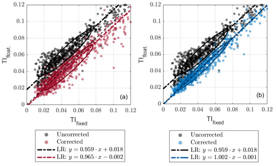
Figure 8.
Comparison between the motion-corrected floating-lidar (basic and enhanced models) and the fixed-lidar TI. (a) Basic model of Table 1 and (b) enhanced model. (Black dot-dashed line, both panels) Linear regression (uncorrected) on . (Red dot-dashed line, panel (a)) Linear regression on for the basic model. (Blue dot-dashed line, panel (b)) Linear regression on for the enhanced model. The minor axes of the ellipses delimit the population spread outside of the linear-regression line (see text).
When comparing the correction performance of the enhanced filter with previously published results in the state-of-the-art filter, the filter outperformed other methods [14,24] because of the demonstrated wind tracking capabilities under the different turbulent regimes (Figure 5a and Figure 6b) and convergence in all motion scenarios. Without having access to the lidar internal LoS measurements, the enhanced filter attains similar correction accuracy as the motion compensation algorithm by Kelberlau et al. [21] under similar wave ( deg) and wind conditions ( m/s). Yet, the outstanding feature of the UKF is that it is able to operate in a stand-alone run-time fashion, i.e., with no need to synchronize with the lidar measurement timestamps for data post-processing.
3.4. Method Limitations
First, the results demonstrated in this study are limited to the ZephIR-300 FDWL sounding at a single height. The single-height configuration was chosen in this study for its simplicity when assessing the comparative filter performance between the “basic’’ and the “enhanced’’ models. However, a typical configuration for this type of lidar is multiple-height sounding. Under this configuration, the filter has less information available from each individual measurement height because the observation time is divided into the number of sounding heights. The latter is due to the ZephIR lidar measuring the wind at multiple heights by following a sequential pattern. Therefore, filter performance (which was computed from the one-to-one correspondence between the motion-corrected measurements and the ones from the reference fixed lidar in Figure 8) is expected to degrade with an increasing number of sounding heights. See [50] for an in-depth discussion. A consequence of this poorer performance is that the enhanced filter will continue to be able to take the motion out “on average’’ over time but losing the fine detail of the wind time series.
Second, it is important to highlight that, in contrast to anemometers, continuous-wave focusable lidars measure a temporally- and spatially-averaged version of the wind vector. They assume a uniform wind flow during the lidar scan when retrieving the wind vector by means of the VAD algorithm. Therefore, in the turbulent conditions prevailing in the interference created by wind turbines (e.g., induction effect in the inflow and disturbance in the wake [51]), DWLs cannot provide valid measurements of the wind field [52]. Under these circumstances, the proposed AR and RW wind models are no longer valid for modeling such high turbulent flows, which may lead to filter divergence.
Finally, regarding filter convergence, the enhanced filter demonstrate itself able to successfully correct the corrupted wind measurements under all motional conditions in the mild near-shore scenario of the PdP campaign (FDWL mean translational velociy lower than 0.5 m/s, mean tilt amplitude lower than 3 deg and wave periods longer than 3 s). Provided correct measurement of the FDWL motion attitude by the IMUs (see Nyquist criterion and sampling requirements in Section 2.1), which was always the case, the filter was at all times able to compensate for the motion-corrupted wind. Therefore, rougher conditions such as those occurring in open seas (higher tilt amplitudes about 5 deg and wave periods longer than 2 s [39]) or the hydrodynamics associated with floating offshore wind turbines [53] are not expected to affect the filter performance.
Although future research is to give further insight into harsher sea-wave and wind conditions, preliminary limits of filter convergence were analyzed via simulation. FDWL measurements were simulated from turbulent wind fields generated using the Mann model [54]. The filter was found to be reliable under these extreme motional conditions: mean tilt > 15 deg and mean translational velocity > 2 m/s, provided that correct measurements of the FDWL attitude were input from the IMUs (see Nyquist criterion and sampling requirements in Section 2.1). On the other hand, the filter was unable to track highly turbulent wind fields with TIs higher than ≃30%.
4. Conclusions
Enhanced wind and lidar initial scan phase models for the FDWL motion-correction UKF filter [25] are presented. The novelty of the enhanced filter relies on the superior wind-tracking capabilities of the filter at a 10-min level under different turbulent regimes without having access to the lidar internal LoS measurements, nor to the lidar measurement timestamps for filter synchronization. The new UKF combines an AR wind model with a UCM initial-phase model, which supersedes the basic RW used for both the wind and initial-phase models in the previous filter. In addition, the state-space reformulation of the UKF along with an implementation based on a dual filter enables the fine removal of the motion-induced as well as straightforward processing to be achieved.
Regarding the wind model, it is shown that while the former RW model can follow only up to the first lobe of the wind spectrum, an AR model of order 10 can reproduce high-frequency wind fluctuations up to 0.1 Hz. According to our experiments, the improvement was higher with the increase in the order of the AR process.
With respect to the lidar-scan model, the rotation of the wedge prism used for laser-beam steering is modeled assuming a uniform circular model. Our results demonstrate that this model clearly outperformed the RW model previously used, which inaccurately assumed a random uniform distribution of the initial phase.
As far as filter implementation is concerned, the dual UKF combines two filters working cooperatively (Figure 4): the main filter (UKF1), which is the motion-correction filter itself, and the auxiliary filter (UKF2), which estimates the AR wind-model coefficients. The main filter estimates the true wind-vector (, and ) and the initial scan phase given the AR coefficients estimated by the auxiliary filter, i.e., the IMU-measured 6 DoF motion of the floating lidar and the lidar-measured wind. The prediction step aims at estimating the true wind vector and initial phase prior to the assimilation of the present-time motion-corrupted wind. The innovation step aims at matching the present-time floating-lidar-measured wind vector to the filter-predicted motion-corrupted wind at each recursive cycle of the filter.
The dual-UKF motion-correction performance was validated over the 6–30 June 2013 intensive observation period during the PdP campaign in different wind and motional scenarios using big-data clustering. The enhanced model combination proved itself as the best candidate to address the FDWL motion compensation in all wind and motional scenarios and statistically demonstrated a virtually ideal correction. With reference to the 10 min fixed-lidar data, the improved from 1.62% (floating lidar without motion correction) to −0.07% (with correction), while increased from 0.90 to 0.96, and the improved from 1.87% to 0.58%. Though the superior performance of the enhanced model as compared with the basic one is undeniable, the basic model also provided convergent results and acceptable indicators to correct the FDWL motion in most cases. At a finer level of detail, the enhanced model permitted the over-compensation issue of the basic model to be overcome thanks to its capability to track the high-frequency spectral fluctuations of wind turbulence (Figure 5 and Figure 6). The latter proves the enhanced filter as a better candidate for the measurement of incoming wind disturbances in floating wind turbine control. Feasibility and convergence of the enhanced filter is discussed in Section 3.4.
All in all, this study demonstrates the importance of the accurate modeling of the wind turbulence spectrum, initial scan phase and motion dynamics for the successful removal of motion-induced turbulence in floating-lidar measurements. However, the filter was tested over experimental data measured under mild environmental conditions (Mediterranean shore). Future research is to extend this study to harsher scenarios. Furthermore, a better experimental set-up, having both the reference and the floating lidars beside each other, could help minimize wind-direction-induced errors when computing performance statistics. Finally, the filter needs to be tested with FDWLs configured to measure the wind at multiple heights.
Author Contributions
This work was developed as part of A.S.-B.’s doctoral thesis, supervised by F.R.; FDWL motion-correction RAUKF, A.S.-B.; software development, A.S.-B.; analyses and figures, A.S.-B.; writing—original draft preparation, A.S.-B.; review and editing, F.R.; funding acquisition, F.R.; conceptualization support, F.R.; measurement campaign lead, J.S. All authors have read and agreed to the published version of the manuscript.
Funding
This research project was part of projects PGC2018-094132-B-I00 and MDM-2016-0600 (“CommSensLab” Excellence Unit) funded by Ministerio de Ciencia e Investigación (MCIN)/ Agencia Estatal de Investigación (AEI)/ 10.13039/501100011033/ FEDER “Una manera de hacer Europa”. The work of A. Salcedo-Bosch was supported by grant 2020 FISDU 00455 funded by Generalitat de Catalunya—AGAUR. The European Commission collaborated under projects H2020 ACTRIS-IMP (GA-871115) and H2020 ATMO-ACCESS (GA-101008004). The European Institute of Innovation and Technology (EIT), KIC InnoEnergy project NEPTUNE (call FP7), supported the measurement campaigns.
Institutional Review Board Statement
Not applicable.
Informed Consent Statement
Not applicable.
Data Availability Statement
Data are available from the authors.
Acknowledgments
The Ph.D. stay of A. Salcedo-Bosch with Jakob Mann, Charlotte B. Hasager and A. Peña at Denmark Technical University (DTU), Wind Energy, 9 January 2022–13 March 2022, as well as participation in DTU Summer School 2020, is gratefully acknowledged.
Conflicts of Interest
The authors declare no conflict of interest.
Sample Availability
Samples are available from the authors.
Abbreviations
The following abbreviations are used in this manuscript:
| AR | Auto-regressive |
| DoF | Degrees of freedom |
| DOAJ | Directory of open access journals |
| DWL | Doppler wind lidar |
| FDWL | Floating Doppler wind lidar |
| HWS | Horizontal wind speed |
| IMU | Inertial measurement unit |
| LD | Linear dichroism |
| LoS | Line of sight |
| NED | North–east–down |
| metmast | Meteorological mast |
| MDPI | Multidisciplinary Digital Publishing Institute |
| PdP | Pont del Petroli |
| PSD | Power spectral density |
| PSLL | Primary-to-secondary lobe level |
| RW | Random walk |
| SV | Spatial variation |
| TI | Turbulence intensity |
| TLA | Three-letter acronym |
| UCM | Uniform circular motion |
| UKF | Unscented Kalman filter |
| UKF1 | Main filter |
| UKF2 | Auxiliary filter |
| VAD | Velocity–azimuth display |
| VWS | Vertical wind speed |
| WD | Wind direction |
Appendix A. UKF Summary
Here, we briefly summarize the foundations of the UKF as given in [55]. The reader is asked to refer to this reference for extensive details and programming tips.
The unscented Kalman filter is a Kalman filter variety for highly non-linear systems. The UKF approximates the state-vector distribution by means of the unscented transform (UT). The UT is a methodology to approximate the statistics of a random variable that experiences a non-linear transformation. To this end, a minimum set of sample points (so-called sigma-points) representative of random variable’s mean and covariance is selected. This set of sigma-points is selected as follows:
where N is the dimension of vector . Therefore, a set of points is selected, and has dimensions.
Then, the sigma-points are propagated through non-linear function (Equation (4)), and a new set of transformed sigma-points is obtained. This is formulated as follows:
The new set of sigma-points is representative of the transformed random variable statistics (up to the third order for Gaussian variables). In order to approximate the random variable mean, , and covariance, , a weighted average of the sigma-points is carried out, as follows:
where is the i-th sigma-point, and and are the weights defined as follows:
where is a design parameter and is usually set to for Gaussian distributions.
The UKF makes use of the UT to carry out the prediction and innovation steps of the Kalman filter recursive algorithm. The UKF algorithm is almost identical to the one used in the plain Kalman filter; however, the and (Equation (4)) transformations are carried out by means of the UT. Algorithm A1 below, summarizes the UKF recursive algorithm steps. is the initial-state vector; is the expected initial-state vector; L is the state-vector dimension; and , and are the estimation-error, process-noise and measurement-noise covariance matrices. These matrices are adaptively updated (see Equation (10).
| Algorithm A1 UKF algorithm [55]. |
|
References
- Offshore Wind in Europe Key Trends and Statistics 2019; Technical Report; WindEurope: Brussels, Belgium, 2020.
- Gutiérrez Antuñano, M.A. Doppler wind LIDAR Systems Data Processing and Applications: An Overview Towards Developing the New Generation of Wind Remote-Sensing Sensors for Off-Shore Wind Farms. Ph.D. Thesis, UPC, Barcelona, Spain, 2019. [Google Scholar]
- Kost, C.; Schlegl, T. Levelized Cost of Electricity Renewable Energy Technologies; Technical Report; Fraunhofer Institut for Solar Energy Systems ISE: Freiburg, Germany, 2018. [Google Scholar]
- IRENA. Technical Report, Renewable Power Generation Costs in 2020, Abu Dhabi. 2020. Available online: https://www.irena.org/publications/2021/Jun/Renewable-Power-Costs-in-2020 (accessed on 26 April 2022).
- Pichugina, Y.; Banta, R.; Brewer, W.; Sandberg, S.; Hardesty, R. Doppler Lidar–Based Wind-Profile Measurement System for Offshore Wind-Energy and Other Marine Boundary Layer Applications. J. Appl. Meteorol. Climatol. 2012, 51, 327–349. [Google Scholar] [CrossRef]
- Courtney, M.S.; Hasager, C.B. Remote sensing technologies for measuring offshore wind. In Offshore Wind Farms; Elsevier: Amsterdam, The Netherlands, 2016; Chapter 4; pp. 59–82. [Google Scholar]
- Gottschall, J.; Gribben, B.; Stein, D.; Würth, I. Floating lidar as an advanced offshore wind speed measurement technique: Current technology status and gap analysis in regard to full maturity. WIREs Energy Environ. 2017, 6, e250. [Google Scholar] [CrossRef]
- Carbon Trust. Carbon Trust Offshore Wind Accelerator Roadmap for the Commercial Acceptance of Floating LiDAR Technology; Technical Report; Carbon Trust: London, UK, 2018. [Google Scholar]
- Bischoff, O.; Wurth, I.; Gottschall, J.; Gribben, B.; Hughes, J.; Stein, D.; Verhoef, H. Recommended Practices for Floating Lidar Systems. Technical Report, IEA Wind Task 32; IEA: Paris, France, 2016. [Google Scholar]
- Gutiérrez, M.A.; Tiana-Alsina, J.; Bischoff, O.; Cateura, J.; Rocadenbosch, F. Performance evaluation of a floating doppler wind lidar buoy in mediterranean near-shore conditions. In Proceedings of the 2015 IEEE International Geoscience and Remote Sensing Symposium (IGARSS), Milan, Italy, 26–31 July 2015. [Google Scholar]
- Gutierrez-Antunano, M.A.; Tiana-Alsina, J.; Rocadenbosch, F.; Sospedra, J.; Aghabi, R.; Gonzalez-Marco, D. A wind-lidar buoy for offshore wind measurements: First commissioning test-phase results. In Proceedings of the 2017 IEEE International Geoscience and Remote Sensing Symposium (IGARSS-2017), Fort Worth, TX, USA, 23–28 July 2017; IEEE: Fort Worth, TX, USA, 2017; pp. 1607–1610. [Google Scholar] [CrossRef]
- Schuon, F.; González, D.; Rocadenbosch, F.; Bischoff, O.; Jané, R. KIC InnoEnergy Project Neptune: Development of a Floating LiDAR Buoy for Wind, Wave and Current Measurements. In Proceedings of the DEWEK 2012 German Wind Energy Conference, Bremen, Germany, 7–8 November 2012; DEWEK: Bremen, Germany, 2012. [Google Scholar]
- Mathisen, J.P. Measurement of wind profile with a buoy mounted lidar. Energy Procedia 2013, 12, 154. [Google Scholar]
- Gutiérrez-Antuñano, M.; Tiana-Alsina, J.; Salcedo, A.; Rocadenbosch, F. Estimation of the Motion-Induced Horizontal-Wind-Speed Standard Deviation in an Offshore Doppler Lidar. Remote Sens. 2018, 10, 2037. [Google Scholar] [CrossRef]
- Ali Shah, K.; Meng, F.; Li, Y.; Nagamune, R.; Zhou, Y.; Ren, Z.; Jiang, Z. A synthesis of feasible control methods for floating offshore wind turbine system dynamics. Renew. Sustain. Energy Rev. 2021, 151, 111525. [Google Scholar] [CrossRef]
- Tiana-Alsina, J.; Gutiérrez, M.A.; Würth, I.; Puigdefàbregas, J.; Rocadenbosch, F. Motion compensation study for a floating doppler wind lidar. In Proceedings of the 2015 IEEE International Geoscience and Remote Sensing Symposium (IGARSS-2015), Milan, Italy, 26–31 July 2015; pp. 5379–5382. [Google Scholar]
- Salcedo-Bosch, A.; Gutierrez-Antunano, M.A.; Tiana-Alsina, J.; Rocadenbosch, F. Floating Doppler Wind Lidar Measurement of Wind Turbulence: A Cluster Analysis. In Proceedings of the 2020 IEEE International Geoscience and Remote Sensing Symposium (IGARSS-2020), Waikoloa, HI, USA, 26 September–2 October 2020. [Google Scholar]
- Bardal, L.M.; Sætran, L. Influence of turbulence intensity on wind turbine power curves. Energy Procedia 2017, 137, 553–558. [Google Scholar] [CrossRef]
- Clifton, A.; Courtney, M. 15. Ground-Based Vertically Profiling Remote Sensing for Wind Resource Assessment; Technical Report; IEA Wind Expert Group Study on Recommended Practices; IEA Wind: Paris, France, 2013. [Google Scholar]
- Clifton, A.; Wagner, R. Accounting for the effect of turbulence on wind turbine power curves. J. Phys. Conf. Ser. 2014, 524, 012109. [Google Scholar] [CrossRef]
- Kelberlau, F.; Neshaug, V.; Lønseth, L.; Bracchi, T.; Mann, J. Taking the Motion out of Floating Lidar: Turbulence Intensity Estimates with a Continuous-Wave Wind Lidar. Remote Sens. 2020, 12, 898. [Google Scholar] [CrossRef]
- Wolken-Möhlmann, G.; Lilov, H.; Lange, B. Simulation of motion induced measurement errors for wind measurements using LIDAR on floating platforms. In Proceedings of the 15th International Symposium for the Advancement of Boundary-layer Remote Sensing (ISARS), Paris, France, 28–30 June 2010; pp. 28–30. [Google Scholar]
- Pitter, M.; Burin des Roziers, E.; Medley, J.; Mangat, M.; Slinger, C.; Harris, M. Performance Stability of Zephir in High Motion Enviroments: Floating and Turbine Mounted; Technical Report; ZephIR: Barcelona, Spain, 2014. [Google Scholar]
- Gutiérrez-Antuñano, M.A.; Tiana-Alsina, J.; Rocadenbosch, F. Performance evaluation of a floating lidar buoy in nearshore conditions. Wind Energy 2017, 20, 1711–1726. [Google Scholar] [CrossRef]
- Salcedo-Bosch, A.; Rocadenbosch, F.; Sospedra, J. A Robust Adaptive Unscented Kalman Filter for Floating Doppler Wind-LiDAR Motion Correction. Remote Sens. 2021, 13, 4167. [Google Scholar] [CrossRef]
- Bischoff, O.; Schlipf, D.; Würth, I.; Cheng, P. Dynamic Motion Effects and Compensation Methods of a Floating Lidar Buoy. In Proceedings of the EERA DeepWind 2015 Deep Sea Offshore Wind Conference, Trondheim, Norway, 3–5 February 2015. [Google Scholar]
- Gottschall, J.; Wolken-Möhlmann, G.; Viergutz, T.; Lange, B. Results and conclusions of a floating-lidar offshore test. Energy Procedia 2014, 53, 156–161. [Google Scholar] [CrossRef]
- Gottschall, J.; Lilov, H.; Wolken-Möhlmann, G.; Lange, B. Lidars on floating offshore platforms about the correction of motion-induced lidar measurement errors. In EWEA 2012 Proceedings; The European Wind Energy Association, Ed.; EWEA: Lisbon, Portugal, 2012. [Google Scholar]
- Schlipf, D.; Rettenmeier, A.; Haizmann, F.; Hofsäß, M.; Courtney, M.; Cheng, P.W. Model based wind vector field reconstruction from lidar data. In Proceedings of the 11th German Wind Energy Conference DEWEK, Bremen, Germany, 7–8 November 2012. [Google Scholar]
- Robert Grover, R.; Y.C. Hwang, P. Introduction to Random Signals and Kalman Filtering: With MATLAB Exercises, 4th ed.; Wiley: Hoboken, NJ, USA, 2012. [Google Scholar]
- Shannon, C. Communication in the Presence of Noise. Proc. IRE 1949, 37, 10–21. [Google Scholar] [CrossRef]
- Slinger, C.; Harris, M. Introduction to Continuous-Wave Doppler Lidar. Available online: http://breeze.colorado.edu/ftp/RSWE/Chris_Slinger.pdf (accessed on 21 July 2021).
- Schlipf, D. Lidars and wind turbine control. In Remote Sensing for Wind Energy; Number 0084(EN) in DTU Wind Energy E; DTU Wind Energy: Denmark, Roskilde, 2015. [Google Scholar]
- Olondriz, J.; Elorza, I.; Trojaola, I.; Pujana, A.; Landaluze, J. On the effects of basic platform design characteristics on floating offshore wind turbine control and their mitigation. J. Phys. Conf. Ser. 2016, 753, 052008. [Google Scholar] [CrossRef]
- James, J.E.; Hooper, W.P. Beam Pointing Stabilization for a Shipboard Volume Imaging Lidar. Nav. Res. Lab. 1995, 20375–25320. [Google Scholar]
- Proakis, J.; Manolakis, D. Digital Signal Processing, 4th ed.; Prentice Hall: Hoboken, NJ, USA, 2006. [Google Scholar]
- Smith, D.A.; Mehta, K.C. Investigation of stationary and nonstationary wind data using classical Box-Jenkins models. J. Wind Eng. Ind. Aerodyn. 1993, 49, 319–328. [Google Scholar] [CrossRef]
- Wan, E.A.; Van Der Merwe, R. The unscented Kalman filter for nonlinear estimation. In Proceedings of the IEEE 2000 Adaptive Systems for Signal Processing, Communications, and Control Symposium (Cat. No.00EX373), Lake Louise, AB, Canada, 4 October 2000; pp. 153–158. [Google Scholar] [CrossRef]
- Salcedo-Bosch, A.; Rocadenbosch, F.; Gutiérrez-Antuñano, M.A.; Tiana-Alsina, J. Estimation of Wave Period from Pitch and Roll of a Lidar Buoy. Sensors 2021, 21, 1310. [Google Scholar] [CrossRef]
- Rocadenbosch, F.; Soriano, C.; Comerón, A.; Baldasano, J.M. Lidar inversion of atmospheric backscatter and extinction-to-backscatter ratios by use of a Kalman filter. Appl. Opt. 1999, 38, 3175–3189. [Google Scholar] [CrossRef] [PubMed]
- Araújo da Silva, M.P.; Rocadenbosch, F.; Tanamachi, R.L.; Saeed, U. Motivating a Synergistic Mixing-Layer Height Retrieval Method Using Backscatter Lidar Returns and Microwave-Radiometer Temperature Observations. IEEE Trans. Geosci. Remote Sens. 2022, 60, 1–18. [Google Scholar] [CrossRef]
- Araújo da Silva, M.P.; Rocadenbosch, F.; Farré-Guarné, J.; Salcedo-Bosch, A.; González-Marco, D.; Peña, A. Assessing Obukhov Length and Friction Velocity from Floating Lidar Observations: A Data Screening and Sensitivity Computation Approach. Remote Sens. 2022, 14, 1394. [Google Scholar] [CrossRef]
- Jeffreys, H.; Taylor, G.I. On the formation of water waves by wind. Proc. R. Soc. Lond. Ser. A Contain. Pap. Math. Phys. Character 1925, 107, 189–206. [Google Scholar] [CrossRef]
- He, Y.; Fu, J.; Chan, P.W.; Li, Q.; Shu, Z.; Zhou, K. Reduced Sea-Surface Roughness Length at a Coastal Site. Atmosphere 2021, 12, 991. [Google Scholar] [CrossRef]
- Stull, R.B. An Introduction to Boundary Layer Meteorology; Kluwer Academic Publishers: Dordrecht, The Netherlands, 1988. [Google Scholar]
- Monin, A. Basic laws of turbulent mixing in the surface layer of the atmosphere. Contrib. Geophys. Inst. Acad. Sci. USSR 1954, 151, e187. [Google Scholar]
- Türk, M.; Emeis, S. The dependence of offshore turbulence intensity on wind speed. J. Wind Eng. Ind. Aerodyn. 2010, 98, 466–471. [Google Scholar] [CrossRef]
- MacEachern, C. İlhami Yıldız. 1.16 Wind Energy. In Comprehensive Energy Systems; Dincer, I., Ed.; Elsevier: Oxford, UK, 2018; pp. 665–701. [Google Scholar] [CrossRef]
- Lange, B.; Larsen, S.; Højstrup, J.; Barthelmie, R. Importance of thermal effects and sea surface roughness for offshore wind resource assessment. J. Wind Eng. Ind. Aerodyn. 2004, 92, 959–988. [Google Scholar] [CrossRef]
- Salcedo-Bosch, A.; Rocadenbosch, F.; Sospedra, J. On Adaptive Unscented Kalman Filtering for Floating Doppler Wind-Lidar Motion Correction: Effect of the Number of Lidar Measurement Heights. In Proceedings of the 2022 IEEE International Geoscience and Remote Sensing Symposium (IGARSS), Kuala Lumpur, Malaysia, 17–22 July 2022. [Google Scholar]
- Micallef, D.; Rezaeiha, A. Floating offshore wind turbine aerodynamics: Trends and future challenges. Renew. Sustain. Energy Rev. 2021, 152, 111696. [Google Scholar] [CrossRef]
- Gottschall, J. Wake Measurements with Lidar. In Handbook of Wind Energy Aerodynamics; Stoevesandt, B., Schepers, G., Fuglsang, P., Yuping, S., Eds.; Springer International Publishing: Cham, Switzerland, 2020; pp. 1–18. [Google Scholar] [CrossRef]
- Gao, Z.t.; Feng, X.y.; Zhang, Z.t.; Liu, Z.l.; Gao, X.x.; Zhang, L.j.; Li, S.; Li, Y. A brief discussion on offshore wind turbine hydrodynamics problem. J. Hydrodyn. 2022, 34, 15–30. [Google Scholar] [CrossRef]
- Mann, J. Wind field simulation. Probabilistic Eng. Mech. 1998, 13, 269–282. [Google Scholar] [CrossRef]
- Julier, S.J.; Uhlmann, J.K. New extension of the Kalman filter to nonlinear systems. In Signal Processing, Sensor Fusion, and Target Recognition VI; Kadar, I., Ed.; International Society for Optics and Photonics; SPIE: Bellingham, WA, USA, 1997; Volume 3068, pp. 182–193. [Google Scholar] [CrossRef]
Publisher’s Note: MDPI stays neutral with regard to jurisdictional claims in published maps and institutional affiliations. |
© 2022 by the authors. Licensee MDPI, Basel, Switzerland. This article is an open access article distributed under the terms and conditions of the Creative Commons Attribution (CC BY) license (https://creativecommons.org/licenses/by/4.0/).