RFI Detection and Mitigation for Advanced Correlators in Interferometric Radiometers

Abstract

This work presents the first RFI detection and mitigation algorithm for the interferometric radiometers that will be implemented in its correlator unit. The algorithm operates in the time and frequency domains, applying polarimetric and statistical tests in both domains, and exhibiting a tunable and arbitrary low probability of false alarm. It is scalable to a configurable number of receivers, and it is optimized in terms of quantization bits and the implementation of the cross-correlations in the time or frequency domains for hardware resource saving. New features of this algorithm are the computation of the Stokes parameters per frequency bin in the Short-Time Fourier Transform and a new parameter called Polarimetric Kurtosis. If RFI is detected in one domain or in both, it is removed using the calculated blanking masks. The optimum algorithm parameters are computed, such as length of the FFTs, the threshold selection for a given probability of false alarm, and the selection of the blanking masks. Last, an important result refers to the application of Parseval’s theorem for the computation of the cross-correlations in the frequency domain, instead of in the time domain, which is more efficient and leads to smaller errors even when using moderate quantization levels. The algorithm has been developed in the framework of the ESA’s technology preparation for a potential L-band radiometer mission beyond SMOS. However, it is also applicable to (polarimetric) real aperture radiometers, and its performance would improve if more than one bit is used in the signal quantization.

1. Introduction

Radio Frequency Interference (RFI) signals are undesired electromagnetic emissions that can degrade the performance of any receiver. Nowadays, the concern about the RFI phenomenon is increasing due to the high number of RFI occurrences detected, and this problem is expected to grow even more in the future because of the pervasive use and abuse of wireless technologies around the world (Figure 1). RFI signals are either those illegally emitted at bands reserved for passive observations (in-band effect) or those that are legally emitted in adjacent bands; however, a fraction of their power leaks into the bandwidth of the radiometer (near-band effect) or even a harmonic emission at a much lower frequency band. The origins of these RFI signals can be of very different natures: they can be lower harmonics, inter-modulation products, out-of-band emissions, or even intentional emissions designed to override a particular frequency band. According to [1], the allocated bands provide a statutory protection, with no guarantee against interference occurrences from accidental out-of-band emissions or intentional jamming. Therefore, RFI has become a dangerous threat for passive remote sensing and, in particular, for Microwave Radiometry (MWR) as microwave radiometers have high sensitivity requirements, of the order of a Kelvin, or less [2].

In Ref [4], a comprehensive literature review on RFI detection and mitigation (D/M) techniques in Earth observation by means of the passive microwave (i.e., radiometry and GNSS-R) is presented. Existing D/M techniques can be classified as parametric (designed to mitigate a particular type RFI signal, e.g., a CW signal) or non-parametric (RFI-type agnostic). These techniques can also be classified according to their domain of operation: time domain, frequency domain, statistical domain, polarimetry domain, or space domain (e.g., direction of arrival followed by beamforming or null-steering antennas). The performance of each technique is highly dependent on the RFI scenario, and the RFI D/M algorithms may combine techniques from several domains to be more effective [5], e.g., time-statistical domains [6], time-frequency domains [7], frequency-statistical domains [8], time-scale domains and Wavelet Packet Decomposition (WPD) [9], signal sub-spaces decomposition (Karhunen–Loève Transform or KLT) [10], Principal Component Analysis or PCA [11], Independent Component Analysis or ICA [12], multi-lag correlations [13], and time-space domains (e.g., adaptive beamforming/null-steering) [14,15].

There are two types of microwave radiometers: real and synthetic aperture ones. They can be single or dual polarization or fully polarimetric if they measure the full Stokes vector [16]. Real aperture radiometers have a single antenna whose beam(s) determines the spatial resolution, and the image is formed by scanning the beam(s). Synthetic aperture radiometers have multiple small antennas, and the complex cross-correlation of the signals collected by each pair of antennas provides a sample of the so-called “visibility function”, which corresponds to a spectral component of the apparent brightness temperature. The image is then formed by Fourier synthesis techniques. Because of the large number of receivers, the complex cross-correlations are typically implemented using very few bits or even just one bit and two-level correlators.

The principles of operation of synthetic aperture radiometers are described in Section “4.6.2.1.2 Synthetic Aperture Radiometers” of [17]. The impact of hard quantization schemes is described in Section “4.6.3.1.3 Sampling Considerations” or in [18], and in the case of ideal error-free 1-bit comparators, an arcsin transfer function must be applied to transform the normalized digital correlation into a normalized analog one, as shown by [19]. This is an important effect that needs to be taken into consideration in the algorithm optimization

In synthetic aperture radiometers, a cooperative RFI detection approach may be considered assuming that the same RFI signal will likely be collected by all antenna elements, as they are physically close. However, although cooperative RFI mitigation may be applied in the simplest time, frequency, and statistical domain algorithms, it is not feasible in other approaches, or in a multi-domain approach. The analysis of RFI in synthetic aperture radiometers was first studied in [20], and it was found that it could be very severe. Therefore, the RFI mitigation must be applied to the signals received from each single antenna element before they are cross-correlated. It is important to note that the dynamic range of the RFI signals that can be mitigated is strongly related to the number of bits used in the quantization process, and the use (or not) of an Automatic Gain Control (AGC) stage. For example, if the number of bits is low and there is a strong RFI, the noise signal to be correlated will be totally masked by the RFI and either the correlation is that of the RFI signal or—if cleaned—the cross-correlation will be zero as the noise signal is under the quantization noise. Moreover, the performance of RFI mitigation techniques after correlation is limited as some of such filtering techniques only allow the removal of abnormally high brightness temperature spots with accurate geo-localization of the RFI source (e.g., [14,21,22]).

In this study, an RFI detection and mitigation algorithm is presented as part of the technology developments towards an SMOS follow-on mission. The algorithm has been conceived to operate on 1-bit quantized signals only, as provided by the receivers connected to each dual-polarization antenna in the interferometric array, but it can also be implemented if softer (i.e., with more bits) quantization schemes are used. The 1-bit quantization is the one that produces the strongest clipping of the amplitude signal and the largest spectrum spread, and it affects the signal auto-correlation, the cross-correlation of two 1-bit quantized signals, the Fourier transform of the cross-correlation function, and the variance of the measurements (i.e., effective integration time smaller than the integration time) [19,23]. As the amplitude information is lost, the instantaneous power information is also lost. Even though the 1-bit quantization makes the RFI mitigation task more difficult and less performant, some alternatives can be applied. In particular, two new RFI mitigation approaches are proposed in this study: the calculation of the Stokes parameters per frequency bin in the Short-Time Fourier Transform (STFT) and the Polarimetric Kurtosis, which are explained in the next section.

2. Materials and Methods

The proposed inputs for the new RFI detection and mitigation algorithm correspond to the outputs of the new receivers conceived for the SMOS follow-on mission. These include:

• X_In, X_Qn, Y_In, Y_Qn: four 1-bit data streams per receiver element n (from n = 1...N_receivers) at 57.69375 MHz, X/Y being the polarization, and I/Q the in-phase/quadrature components;
• X_Pn, Y_Pn: two multi-bit Power Measurement System (PMS) streams per receiver element n (from n = 1...N_receivers) and per polarization at ~28 kS/s.

The proposed algorithm is fully tunable, even while in orbit, and some configurable parameters are:

• N is the number of samples per integration period. In this study, N = 11,538,432, corresponding to an integration time of ~200 ms at the clock sampling frequency.
• K is the number of points of the Fourier transform or the number of points in the spectrum. K is an optimization parameter that can be reduced to a smaller power-of-two number during the implementation phase, if needed for Field-Programmable Gate Array (FPGA) resource utilization optimization.
• M is the number of time segments of the Short-Time Fourier Transform (STFT) in which the signal is divided. It is defined as M = γ·N/K, where γ is the windowing factor. As will be shown in the next section, γ = 2, which is the minimum windowing factor necessary to apply a non-rectangular window function.
• R_tot is the total number of receivers of the system.
• R_avg is the number of receivers that are averaged in the RFI detection process. It will be assumed that R_avg = R_tot. In the case of a real aperture radiometer, R_avg = R_tot = 1.
• ${\alpha }_{th}^{}$ is the detection threshold for statistical and polarimetry metrics to determine whether an RFI signal is present or not, and it controls the probability of detection and the probability of false alarm. The parameter ${\alpha }_{th}^{}$ may take three different specific values: ${\alpha }_{th}^{time}$ for temporal moments, ${\alpha }_{th}^{freq}$ for spectral moments, and ${\alpha }_{th}^{all}$ for all-signal moments.
• ${\beta }_{th}^{}$ is the maximum blanking threshold. The RFI mitigation is based on the excision of the contaminated samples out of the set of all transformed samples. The RFI mitigation operates efficiently if a reduced number of samples contain the largest fraction of the RFI power.

2.1. RFI Detection and Mitigation Algorithm Description

Figure 2 shows the overall block diagram of the proposed RFI mitigation algorithm. After an initial windowing to reduce the Gibbs effect associated with the truncation of the data streams, the signal spectrum is computed (FFT). Calibration measurements are acquired in RFI-free conditions and allow the inferring of the receiver’s chain frequency response, which will have to be compensated in subsequent measurements. Equalization is performed during normal acquisitions, which may or may not be affected by RFI, to compensate for the receiver’s frequency response. Once the incoming signal’s spectrum has been whitened (i.e., “flattened” to look like Additive White Gaussian Noise—AWGN—in RFI-free conditions), statistical and polarimetric tests are applied in both the time and the frequency domains to detect the presence of RFI. When RFI is detected in one of these domains using any of the techniques, a blanking mask is calculated for either the time or frequency domains.

The outputs of this RFI mitigation algorithm contain both the final and the intermediate products in the form of the averaged unmitigated and mitigated PMS measurements and the computed blanking masks that will be used to mitigate the RFI prior to the correlator.

In the following subsections, each of the blocks is described.

2.1.1. Windowing

The resolutions in the temporal domain ${\mathsf{\sigma }}_t$ and in the frequency domain ${\mathsf{\sigma }}_f$ are related and constrained by the so-called Gabor limit [24].

$${\mathsf{\sigma }}_t·{\mathsf{\sigma }}_f\ge \frac{1}{4\pi }$$

(1)

The selection of the window coefficients determines the amount of spectral leakage in the Fourier transform output. The square root Hamming window function (Equation (2)) has been selected for this application because it provides a good trade-off between frequency resolution and side-lobe rejection, and it can fulfil the squared perfect reconstruction condition of Equation (3). The window function is defined as:

$$w\left[k\right]=\sqrt{\frac{1}{2}\left[1-\frac{1-\beta }{\beta }cos\left(\frac{2\pi k}{K}\right)\right]},\beta =\frac{25}{46},0\le k<K,$$

(2)

In order to reconstruct the signal properly, the signal has to be windowed at least every K/2 samples. This makes the windowing factor γ, mentioned in the previous section, equal to 2. Setting this value larger than 2 may be helpful for the signal reconstruction in some cases, at the expense of increasing the required computational resources. However, the square root Hamming window function fulfills the following condition:

$$w^2\left[k\right]+w^2\left[k-\frac{K}{2}\right]=1,$$

(3)

therefore, windowing the input signal every K/2 sample is enough to reconstruct the signal back to the time domain.

2.1.2. Spectral Computation

The Short-Time Fourier Transform (STFT) is the most used technique for RFI excision. The signal is filtered in the time-frequency space in order to remove the RFI components before being transformed back to the time domain (Figure 3, left).

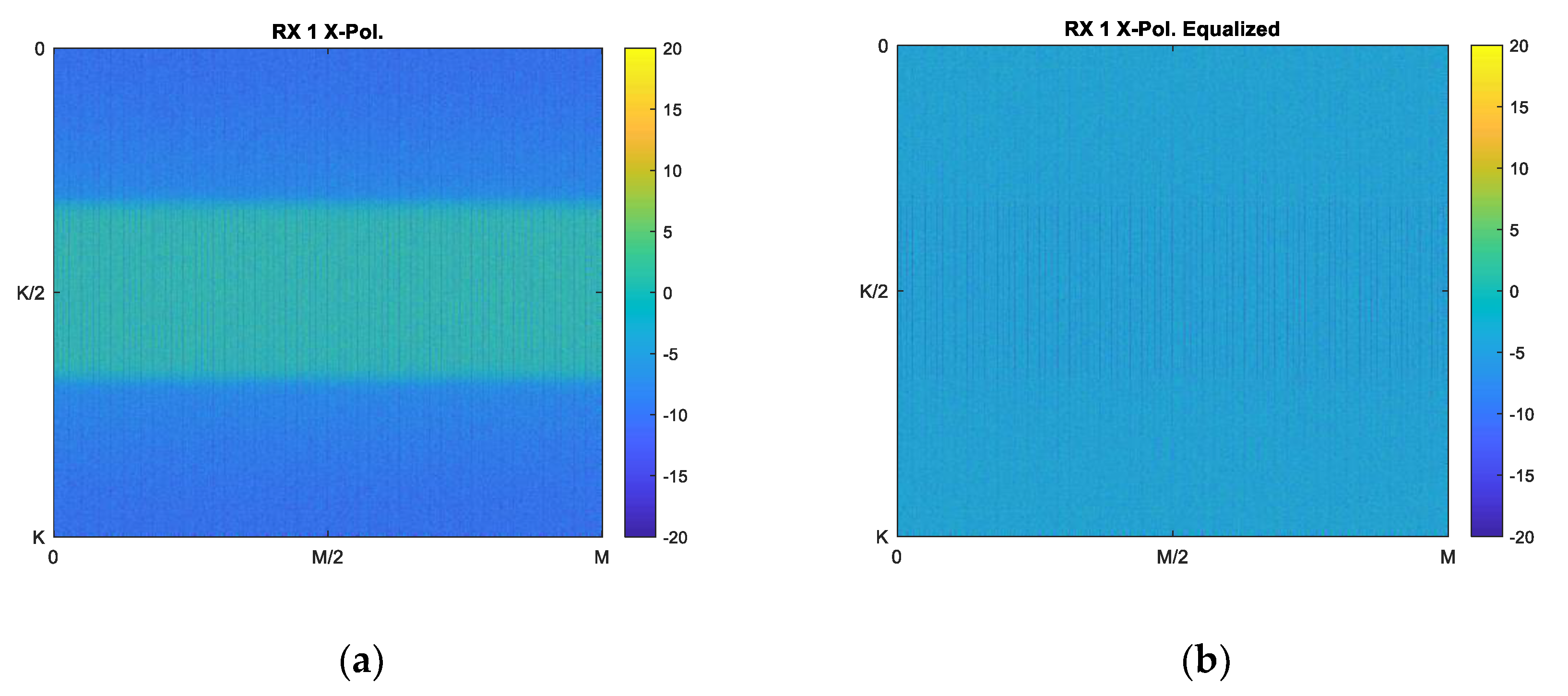
2.1.3. Calibration and Equalization

Calibration and equalization are two stages needed to compensate for the effects of the non-flat frequency response of the receiver when applying some of the RFI mitigation techniques considered in this algorithm, such as cross-spectrum kurtosis or polarimetry. The calibration frequency responses of $Z_r^{cal}\left[k\right]$, with Z = X or Y and r being the receiver number, are calculated as:

$$Z_r^{cal}\left[k\right]=\sqrt{\frac{1}{M}{\displaystyle \sum }_{m=0}^{M-1}{\left|Z_r^{}\left[m,k\right]\right|}^2}$$

(4)

where M is the number of STFTs being averaged, and the equalized frequency responses $Z_r^{eq}\left[k\right]$ are:

$$Z_r^{eq}\left[m,k\right]=\frac{Z_r^{}\left[m,k\right]}{Z_r^{cal}\left[k\right]}.$$

(5)

Note that the normalization is performed in the complex values instead of a power in order to keep the power balance among the different polarizations and receivers. Note also that the spectral calibration is particular for each receiver and polarization as the receiving channels are different. The calibration and equalization results are illustrated graphically in Figure 3, right, for a sample receiver.

Time and frequency decomposition, calibration, and equalization must be performed for each received signal. However, under some assumptions, such as that the RFI pulses are received in the same samples at each receiver (determined by the array size and the off-boresight direction of arrival) or that the frequencies or frequency band of the RFI signals at each receiver are equal, the number of STFTs to be performed may be reduced, even down to 1 in the most extreme case.

2.1.4. Statistic and Polarimetry Tests

The proposed RFI detection algorithm is based on the calculation of some statistical and polarimetric moments over the aggregated time-frequency bins of the different receivers of the system.

• Stokes Parameters

The definition of the modified Stokes parameters for microwave radiometry can be combined with the multi-receiver approach, obtaining an averaged squared Stokes vector S’[m,k] per each bin of the STFT, as follows:

$$S^{\prime }\left[m,k\right]=\left[\begin{array}{c}\begin{array}{c}{s}_1^2\left[m,k\right]\\ s_2^2\left[m,k\right]\end{array}\\ \begin{array}{c}{s}_3^2\left[m,k\right]\\ s_4^2\left[m,k\right]\end{array}\end{array}\right]=\frac{1}{R_{avg}}{{\displaystyle \sum }}_{r=1}^{R_{avg}}\left[\begin{array}{c}\begin{array}{c}{\left|X_r^{eq}\left[m,k\right]\right|}^4\\ {\left|Y_r^{eq}\left[m,k\right]\right|}^4\end{array}\\ \begin{array}{c}4{\left(Re\left\{X_r^{eq}\left[m,k\right]·{\left(Y_r^{eq}\left[m,k\right]\right)}^{*}\right\}\right)}^2\\ 4{\left(Im\left\{X_r^{eq}\left[m,k\right]·{\left(Y_r^{eq}\left[m,k\right]\right)}^{*}\right\}\right)}^2\end{array}\end{array}\right]$$

(6)

where [m,k] are the time and frequency indices of the bin under evaluation, $\left(s_1, s_2, s_3, s_4\right)$ are the first, second, third, and fourth multi-receiver squared Stokes parameters, respectively, and R_avg is the number of receivers whose outputs are averaged.

• Kurtosis and Polarimetric Kurtosis

Kurtosis is the best statistical-based RFI detection algorithm for almost all kinds of interfering signals, although it is known that it has a blind spot for sinusoidal and chirp interfering signals of the 50% duty cycle, which can be overcome using e.g., the Anderson-Darling technique [25]. When combined with the Fourier transform, it is usually called spectral kurtosis because the statistical test is applied per frequency bin. It can be mathematically computed as the ratio between the fourth central moment of a random variable and the square of its variance (second central moment). However, in practice, as thermal noise is zero-mean, and the hardware has a calibrated DC offset, non-central moments are equivalent and used for the calculation of the kurtosis.

At this time, the new “Polarimetric Kurtosis” observable can be introduced as:

$$\left[\begin{array}{c}\begin{array}{c}{k}_1^{all}\\ k_2^{all}\end{array}\\ \begin{array}{c}{k}_3^{all}\\ k_4^{all}\end{array}\end{array}\right]=\frac{1}{M}·\frac{1}{K}{{\displaystyle \sum }}_{m=0}^{M-1}{{\displaystyle \sum }}_{k=0}^{K-1}\left[\begin{array}{c}\begin{array}{c}{s}_1^2\left[m,k\right]/{\left(p_1^{all}\right)}^2\\ s_2^2\left[m,k\right]/{\left(p_2^{all}\right)}^2\end{array}\\ \begin{array}{c}{s}_3^2\left[m,k\right]/{\left(p_1^{all}·p_2^{all}\right)}^{}\\ s_4^2\left[m,k\right]/{\left(p_1^{all}·p_2^{all}\right)}^{}\end{array}\end{array}\right],$$

(7)

where

$$p_{1,2}^{all}=\frac{1}{R_{avg}}·\frac{1}{M}·\frac{1}{K}{{\displaystyle \sum }}_{r=1}^{R_{avg}}{{\displaystyle \sum }}_{m=0}^{M-1}{{\displaystyle \sum }}_{k=0}^{K-1}{s}_{1,2r}^2\left[m,k\right]$$

(8)

the first and second components ($k_{1,2}^{all}$) are the conventional complex sample kurtosis for the X and Y polarization, respectively, and the third and fourth components ($k_{3,4}^{all}$) are obtained as the ratio between the square of the third and fourth multi-receiver Stokes parameters and the product of the second moments at the X and Y polarizations (Equation (8)). Note that Equation (7) expresses the Polarimetric Kurtosis parameters for the bins within the integration time in both domains.

• Time-Frequency Moments

Once the Polarimetric Kurtosis parameters are defined for “all” bins, it is straightforward to define the same metrics along the time and frequency domains. Instead of averaging all the bins of the STFT together, the integration may be performed in only one of the STFT matrix dimensions, either time or frequency.

If the averaging is performed across the cross-frequency bins, the result can be named as the Temporal Polarimetric Kurtosis:

$$\left[\begin{array}{c}\begin{array}{c}{k}_1^{time}\left[m\right]\\ k_2^{time}\left[m\right]\end{array}\\ \begin{array}{c}{k}_3^{time}\left[m\right]\\ k_4^{time}\left[m\right]\end{array}\end{array}\right]=\frac{1}{K}{\displaystyle \sum }_{k=0}^{K-1}\left[\begin{array}{c}\begin{array}{c}{s}_1^2\left[m,k\right]/{\left(p_1^{time}\left[m\right]\right)}^2\\ s_2^2\left[m,k\right]/{\left(p_2^{time}\left[m\right]\right)}^2\end{array}\\ \begin{array}{c}{s}_3^2\left[m,k\right]/{\left(p_1^{time}\left[m\right]·p_2^{time}\left[m\right]\right)}^{}\\ s_4^2\left[m,k\right]/{\left(p_1^{time}\left[m\right]·p_2^{time}\left[m\right]\right)}^{}\end{array}\end{array}\right],$$

(9)

where

$$p_{1,2}^{time}\left[m\right]=\frac{1}{R_{avg}}·\frac{1}{K}{{\displaystyle \sum }}_{r=1}^{R_{avg}}{{\displaystyle \sum }}_{k=0}^{K-1}{s}_{1,2r}^2\left[m,k\right].$$

(10)

If the averaging is performed across the temporal bins, the result can be named as the Spectral Polarimetric Kurtosis:

$$\left[\begin{array}{c}\begin{array}{c}{k}_1^{freq}\left[k\right]\\ k_2^{freq}\left[k\right]\end{array}\\ \begin{array}{c}{k}_3^{freq}\left[k\right]\\ k_4^{freq}\left[k\right]\end{array}\end{array}\right]=\frac{1}{M}{{\displaystyle \sum }}_{m=0}^{M-1}\left[\begin{array}{c}\begin{array}{c}{s}_1^2\left[m,k\right]/{\left(p_1^{freq}\left[k\right]\right)}^2\\ s_2^2\left[m,k\right]/{\left(p_2^{freq}\left[k\right]\right)}^2\end{array}\\ \begin{array}{c}{s}_3^2\left[m,k\right]/{\left(p_1^{freq}\left[k\right]·p_2^{freq}\left[k\right]\right)}^{}\\ s_4^2\left[m,k\right]/{\left(p_1^{freq}\left[k\right]·p_2^{freq}\left[k\right]\right)}^{}\end{array}\end{array}\right],$$

(11)

where

$$p_{1,2}^{freq}\left[k\right]=\frac{1}{R_{avg}}·\frac{1}{M}{\displaystyle \sum }_{r=1}^{R_{avg}}{\displaystyle \sum }_{m=0}^{M-1}{s}_{1,2r}^2\left[m,k\right].$$

(12)

2.1.5. Computation of the OR/AND Masks

There are two approaches to constructing the blanking masks:

• the OR approach is computed by a tensor-logical OR operation between the vector results of the time and frequency RFI detector, denoted as ∨, whereas
• the AND approach is computed analogously using a tensor-logical AND operation, and it is denoted as ∧.

The OR and AND blanking masks are defined for every Polarimetric Kurtosis metric as:

$$B_{k_p}^{OR}\left[m,k\right]=b_p^{time}\left[m\right]\vee b_p^{freq}\left[k\right]$$

(13)

$$B_{k_p}^{AND}\left[m,k\right]=b_p^{time}\left[m\right]\wedge b_p^{freq}\left[k\right]$$

(14)

with p = 1…4, and:

$$\left[\begin{array}{c}\begin{array}{c}{b}_1^{time}\left[m\right]\\ b_2^{time}\left[m\right]\end{array}\\ \begin{array}{c}{b}_3^{time}\left[m\right]\\ b_4^{time}\left[m\right]\end{array}\end{array}\right]=\left\{\left|\left[\begin{array}{c}\begin{array}{c}{k}_1^{time}\left[m\right]\\ k_2^{time}\left[m\right]\end{array}\\ \begin{array}{c}{k}_3^{time}\left[m\right]\\ k_4^{time}\left[m\right]\end{array}\end{array}\right]-2\right|<{\alpha }_{th}^{time}\right\}$$

(15)

$$\left[\begin{array}{c}\begin{array}{c}{b}_1^{freq}\left[k\right]\\ b_2^{freq}\left[k\right]\end{array}\\ \begin{array}{c}{b}_3^{freq}\left[k\right]\\ b_4^{freq}\left[k\right]\end{array}\end{array}\right]=\left\{\left|\left[\begin{array}{c}\begin{array}{c}{k}_1^{freq}\left[k\right]\\ k_2^{freq}\left[k\right]\end{array}\\ \begin{array}{c}{k}_3^{freq}\left[k\right]\\ k_4^{freq}\left[k\right]\end{array}\end{array}\right]-2\right|<{\alpha }_{th}^{freq}\right\}$$

(16)

In the proposed implementation, a simplification of $B_{k_{3,4}}^{OR/AND}\left[m,k\right]$ (Equations (13) and (14)) for the 3rd and 4th Stokes parameters is used, which consists of flagging an RFI in the polarimetric channels if it is either in the 3rd or in the 4th Stokes parameter, as follows:

$$B_{pol}^{OR}\left[m,k\right]=B_{k_3}^{OR}\left[m,k\right]{{\displaystyle \cap }}^{}{B}_{k_4}^{OR}\left[m,k\right]$$

(17)

$$B_{pol}^{AND}\left[m,k\right]=B_{k_3}^{AND}\left[m,k\right]{{\displaystyle \cap }}^{}{B}_{k_4}^{AND}\left[m,k\right]$$

(18)

The final OR and AND blanking masks are computed by intersecting the statistical and polarimetric masks as:

$$B_{1,2}^{OR}\left[m,k\right]=B_{k_{1,2}}^{OR}\left[m,k\right]{{\displaystyle \cap }}^{}{B}_{pol}^{OR}\left[m,k\right]$$

(19)

$$B_{1,2}^{AND}\left[m,k\right]=B_{k_{1,2}}^{AND}\left[m,k\right]{{\displaystyle \cap }}^{}{B}_{pol}^{AND}\left[m,k\right]$$

(20)

2.1.6. RFI Mitigation

• Signal Blanking

Before applying the blanking mask, either the AND or the OR masks must be selected. While the OR approach maximizes the remaining radiometric signal at the same time as it mitigates the RFI power, the AND one may perform better when the RFI signal is faint in both the time and frequency domains, but it may also excise a significant part of the desired signal. An intermediate metric has to be defined to choose between the AND or the OR approaches in real time. To do so, the fraction of the bins to be mitigated by the OR mask is calculated as:

$${\beta }_{1,2}=\frac{1}{M}·\frac{1}{K}{{\displaystyle \sum }}_{m=0}^{M-1}{{\displaystyle \sum }}_{k=0}^{K-1}{B}_{1,2}^{AND}\left[m,k\right]$$

(21)

consequently, the mitigated STFT can be defined as:

$$Z_r^{mit}\left[m,k\right]=\{\begin{array}{c}\left(Z_r\circ B_z^{OR}\right)\left[m,k\right] if {\beta }_z\ge {\beta }_{th}\\ \left(Z_r\circ B_z^{AND}\right)\left[m,k\right] \mathrm{otherwise}\end{array}$$

(22)

where the input $Z_r$ ($Z_r=X_r \mathrm{or} Y_r$) is the OR blanking mask if ${\beta }_z$ is larger than a threshold value ${\beta }_{th}$ or the AND blanking mask otherwise.

• PMS RFI Mitigation

The mitigation of the power measurements is performed by means of a pulse blanking approach in the time domain. However, as the sensibility of the PMS to detect RFI signals is much worse than for the STFT, instead of using just the instantaneous power value from the PMS to infer the presence or not of RFI, the signal blanking mask is calculated directly from the temporal moments of the Polarimetric Kurtosis ($b_{1,2}\left[m\right]$). In the proposed system, as the samples of the PMS are at ~28 kHz, they must first be resampled at the same rate as that of the temporal bins of the STFT.

The RFI mitigation power factors (${\gamma }_{z_r}$, with Z = X or Y) are calculated for each receiver representing the ratio between the power of the bins after mitigation and before, as follows:

$${\gamma }_{z_r}=\frac{{{\displaystyle \sum }}_{m=0}^{M-1}{{\displaystyle \sum }}_{k=0}^{K-1}{\left|Z_r^{mit}\left[m,k\right]\right|}^2}{{{\displaystyle \sum }}_{m=0}^{M-1}{{\displaystyle \sum }}_{k=0}^{K-1}{\left|Z_r^{}\left[m,k\right]\right|}^2},$$

(23)

and after the mitigation of the corrupted PMS, the sum of the PMS samples that have not been discarded has to be normalized by the gamma factor in order to estimate properly the power in each channel/polarization:

$$P_{z_r}^{mit}={\gamma }_{z_r}·{{\displaystyle \sum }}_{m=0}^{M-1}{P}_{z_r}\left[m\right]·b_{z_r}^{time}\left[m\right]$$

(24)

• RFI Detection Flag

The proposed RFI detection flag is computed as the logical OR between the ‘all-bin’ Polarimetric Kurtosis metrics and the first and second Stokes parameter AND blanking matrices, and it can be expressed as

$$d_{RFI}=\vee \left\{\left|\left[\begin{array}{c}\begin{array}{c}{k}_1^{all}\left[m\right]\\ k_2^{all}\left[m\right]\end{array}\\ \begin{array}{c}{k}_3^{all}\left[m\right]\\ k_4^{all}\left[m\right]\end{array}\end{array}\right]-2\right|>{\alpha }_{th}^{all}\right\}\vee {\vee }_{\forall m,k}\overline{B_1^{AND}\left[m,k\right]}\vee {\vee }_{\forall m,k}\overline{B_2^{AND}\left[m,k\right]}$$

(25)

where ⋁ is a logical vector or operator applied over all the elements of a vector or matrix.

The first element of the logical OR in Equation (25) represents the fact that an RFI signal is detected within the dataset if any part of the Polarimetric Kurtosis deviates more than $\pm {\alpha }_{th}^{all}$ from the theoretical value of 2. The value of ${\alpha }_{th}^{all}$ is selected to set the Constant False Alarm Rate or CFAR ($P_{FA}$ = constant):

$$P_{FA}=1-erf\left(\frac{{\alpha }_{th}}{\raisebox{1ex}{$4$}\!\left/ \!\raisebox{-1ex}{$N$}\right.}\right)$$

(26)

where N is the number of samples.

3. Results

An extensive battery of simulations covering a wide range of parameters, and long enough to be statistically representative, is needed in order to select the optimize the algorithm performance. The following parameters must be optimized:

• K is the number of points of FFT. The initial value of K was 4096, but it was proposed to run simulations with K = 16,384, 4096, 2048, 1024, and 256 and then to select the best K for the default CFAR and β_th.
• α_th is the RFI detection threshold for the statistical and polarimetry metrics: temporal, spectral, and all-bin moments. α_th(P_FA) is obtained mathematically for each value of the CFAR.
• The following CFAR values were simulated for the selected value of K: 10⁻⁸, 10⁻⁶, 10⁻⁴, 10⁻², 0.1, and 0.5.
• β_th is the maximum blanking threshold from 100% to 50%.

Simulations with 1200 realizations containing standard RFI intensity distributions, as provided by Zenithal Blue Technologies (ZBT) and based on SMOS-detected RFI, have been used. Figure 4 shows the actual RFI probability and cumulative density functions for SMOS as measured in 2013 and 2020, as well as the simulated ones.

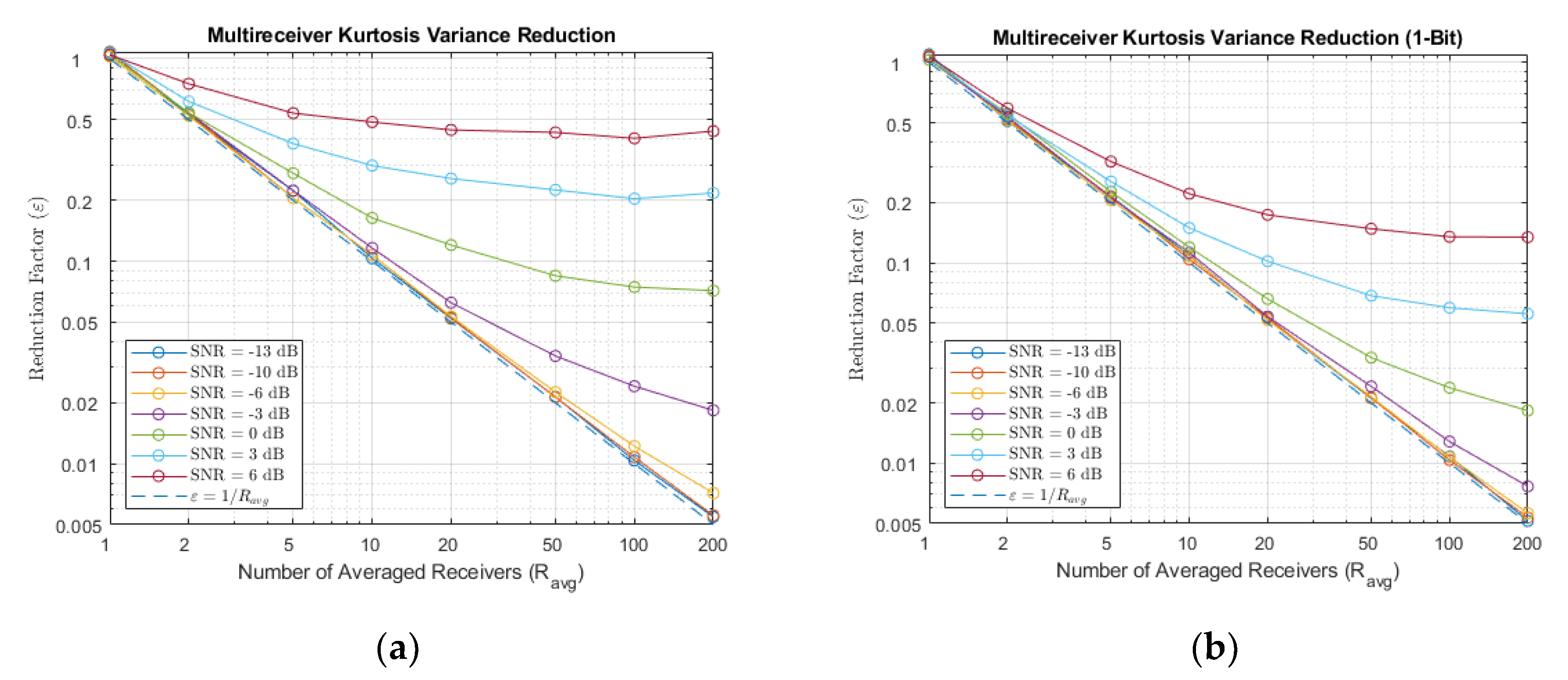
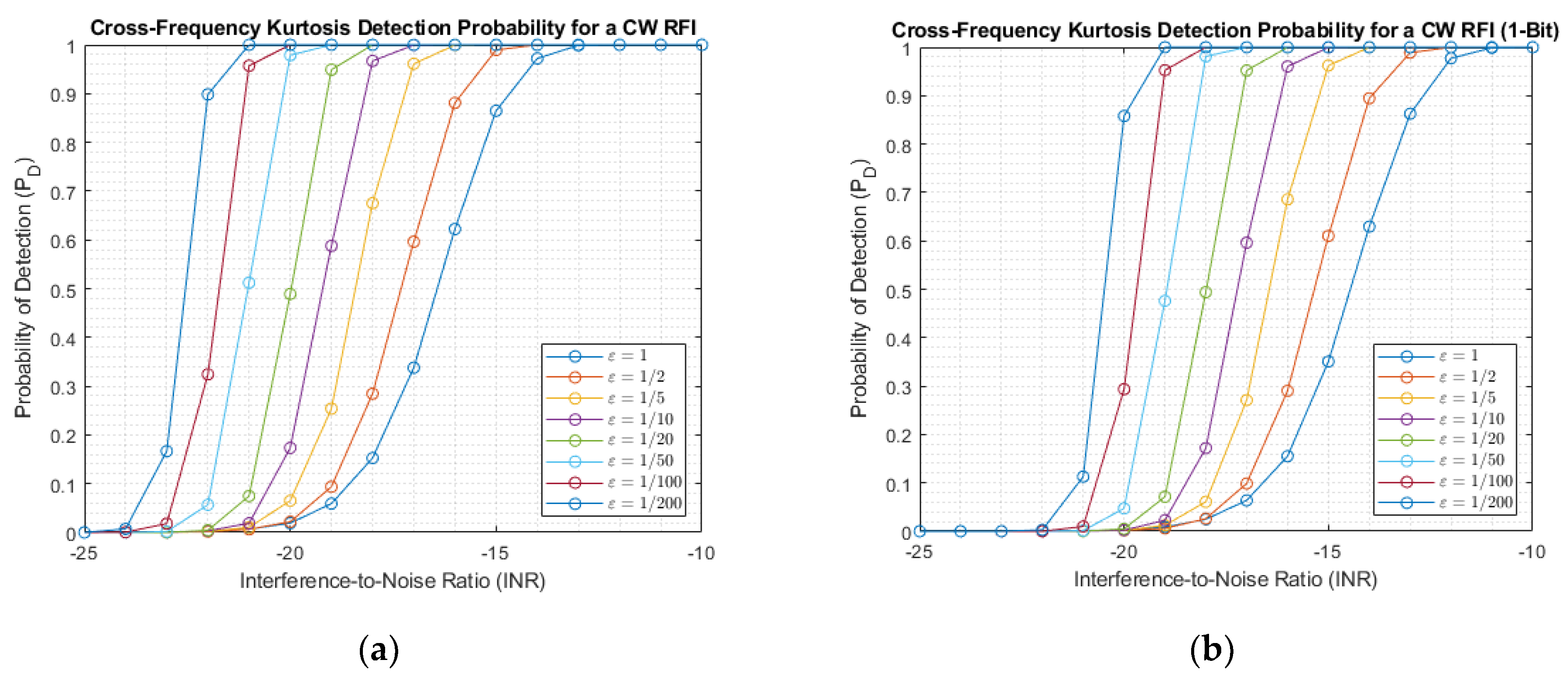
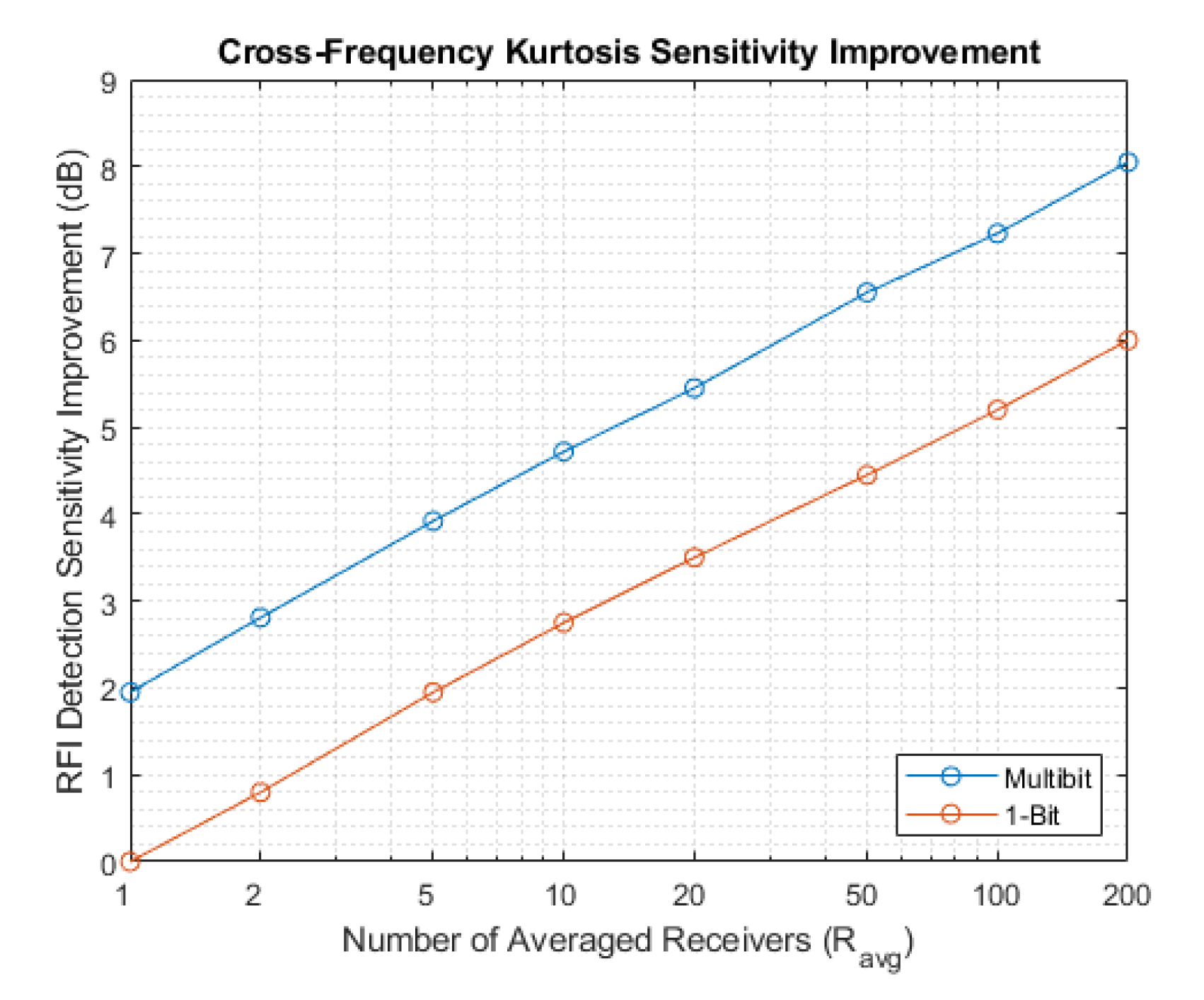
3.1. Sensitivity Performance as a Function of the Number of Averages

An important consideration is the assessment of the sensitivity performance as a function of the number of averaged receivers, assuming, that is, that each receiver has a system to compute the RFI mask and that the input observables are averaged as described before. Figure 5 shows the “reduction of the variance” ($\epsilon$) with respect to R_avg. As can be appreciated in Figure 4, for very low SNR values the variance reduction with respect to R_avg becomes 1/R_avg, but as the SNR increases, the improvement (i.e., the slope) decreases because of the signal correlation. For typical SMOS values, the typical SNR is $SN{R}_{typ}=10·lo{g}_{10}\left({\left|V\right|}_{max}/T_R\right)\approx 10·lo{g}_{10}\left(10 \mathrm{K}/210 \mathrm{K}\right)\approx -13 \mathrm{dB}$, ${\left|V\right|}_{max}$ being the maximum value of the visibility samples or cross-correlation in units of Kelvin, and therefore, the 1/R_avg approximation holds. Note that the use of 1 bit (Figure 5b) instead of multi-bits (Figure 5a) leads to a smaller variance reduction factor, i.e., it is even less sensitive to the SNR.

Figure 6 shows the Probability of Detection (P_D) of RFI vs. the Interference-to-Noise Ratio (INR). It shows a sudden increase above an INR value, which increases with increasing values of $\epsilon$. As compared to the multi-bit case (Figure 6a), in the case of 1-bit quantization (Figure 6b), the plots are shifted ~2 dB towards the right due to larger noise ($10·lo{g}_{10}\left(\sqrt{2.46}\right)\approx 1.95 \mathrm{dB}$). Note that the 2.46 factor is the ratio of the integration time and the effective integration time for the case of 1-bit/2 level correlators [19]. As shown in Figure 7, these ~2 dB are nearly constant as a function of the number of receivers averaged.

3.2. Algorithm Parameter Optimization

The numerical results are presented for the average (M) and the standard deviation (σ) of the mitigation for each value of K (length of the FFT), CFAR, and β_th. The percentages of the mitigated RFI and degraded RFI (the result is worse than no mitigation) are also provided, together with their mean values. In

Table 1. Algorithm performance metrics for K = 4096 and variable CFAR and β_th.

K-FFT 4096	βth 100%			βth 90%			βth 75%			βth 50%
	All #1200	Mitigating (<0)	Degrading (>0)	All #1200	Mitigating (<0)	Degrading (>0)	All #1200	Mitigating (<0)	Degrading (>0)	All #1200	Mitigating (<0)	Degrading (>0)
CFAR 10−8	M: −2.31dB σ: 3.73 dB	%. It. 59.3% M: −4.04 dB	%. It. 7.35% M: 1.14 dB	M: −2.58 dB σ: 5.05 dB	%. It. 56.2% M: −5.48 dB	%. It. 10.4% M: 4.80 dB	M: −2.58 dB σ: 5.05 dB	%. It. 56.2% M: −5.48 dB	%. It. 10.4% M: 4.80 dB	M: −2.58 dB σ: 5.05 dB	%. It. 56.2% M: −5.48 dB	%. It. 10.4% M: 4.80 dB
CFAR 10−6	M: −2.33 dB σ: 3.75 dB	%. It. 60.8% M: −3.97 dB	%. It. 7.65% M: 1.10 dB	M: −2.56 dB σ: 5.11 dB	%. It. 57.5% M: −5.41 dB	%. It. 11.0% M: 4.98 dB	M: −2.56 dB σ: 5.12 dB	%. It. 57.5% M: −5.41 dB	%. It. 11.0% M: 4.98 dB	M: −2.56 dB σ: 5.12 dB	%. It. 57.5% M: −5.41 dB	%. It. 11.0% M: 4.98 dB
CFAR 10−4	M: −2.35 dB σ: 3.82 dB	%. It. 62.2% M: −3.92 dB	%. It. 7.94% M: 1.10 dB	M: −2.52 dB σ: 5.24 dB	%. It. 58.2% M: −5.39 dB	%. It. 11.9% M: 5.24 dB	M: −2.52 dB σ: 5.24 dB	%. It. 58.2% M: −5.39 dB	%. It. 11.9% M: 5.24 dB	M: −2.52 dB σ: 5.24 dB	%. It. 58.2% M: −5.39 dB	%. It. 11.9% M: 5.24 dB
CFAR 10−2	M: 5.88 dB σ: 27.8 dB	%. It. 69.0% M: −3.28 dB	%. It. 28.9% M: 28.16 dB	M: 6.24 dB σ: 29.3 dB	%. It. 63.5% M: −4.98 dB	%. It. 34.4% M: 27.3 dB	M: 6.24 dB σ: 29.3 dB	%. It. 63.5% M: −4.98 dB	%. It. 34.4% M: 27.3 dB	M: 6.24 dB σ: 29.3 dB	%. It. 63.5% M: −4.98 dB	%. It. 34.4% M: 27.3 dB
CFAR 10−1	M: 6.35 dB σ: 28.3 dB	%. It. 73.6% M: −2.86 dB	%. It. 26.4% M: 32.0 dB	M: 12.0 dB σ: 33.0 dB	%. It. 41.3% M: −5.04 dB	%. It. 58.7% M: 23.9 dB	M: 12.0 dB σ: 33.0 dB	%. It. 41.3% M: −5.04 dB	%. It. 58.7% M: 23.9 dB	M: 12.0 dB σ: 33.0 dB	%. It. 41.3% M: −5.04 dB	%. It. 58.7% M: 23.9 dB

,

Table 2. Algorithm performance metrics for K = 2048 and variable CFAR and β_th.

K-FFT 2048	βth 100%			βth 90%			βth 75%			βth 50%
	All #1200	Mitigating (<0)	Degrading (>0)	All #1200	Mitigating (<0)	Degrading (>0)	All #1200	Mitigating (<0)	Degrading (>0)	All #1200	Mitigating (<0)	Degrading (>0)
CFAR 10−8	M: −2.21 dB σ: 3.72 dB	%. It. 57.3% M: −4.02 dB	%. It. 7.31% M: 1.26 dB	M: −2.20 dB σ: 5.20 dB	%. It. 56.2% M: −5.46 dB	%. It. 12.0% M: 5.57 dB	M: −2.20 dB σ: 5.20 dB	%. It. 56.2% M: −5.46 dB	%. It. 12.0% M: 5.57 dB	M: −2.20 dB σ: 5.20 dB	%. It. 56.2% M: −5.46 dB	%. It. 12.0% M: 5.57 dB
CFAR 10−6	M: −2.24 dB σ: 3.77 dB	%. It. 58.4% M: −4.01 dB	%. It. 7.72% M: 1.26 dB	M: −2.19 dB σ: 5.30 dB	%. It. 57.5% M: −5.45 dB	%. It. 12.6% M: 5.72 dB	M: −2.19 dB σ: 5.30 dB	%. It. 57.5% M: −5.45 dB	%. It. 12.6% M: 5.72 dB	M: −2.19 dB σ: 5.30 dB	%. It. 57.5% M: −5.45 dB	%. It. 12.6% M: 5.72 dB
CFAR 10−4	M: −2.20 dB σ: 4.72 dB	%. It. 60.3% M: −3.95 dB	%. It. 8.29% M: 2.09 dB	M: −2.06 dB σ: 6.08 dB	%. It. 58.2% M: −5.39 dB	%. It. 14.1% M: 6.24 dB	M: −2.06 dB σ: 6.08 dB	%. It. 58.2% M: −5.39 dB	%. It. 14.1% M: 6.24 dB	M: −2.06 dB σ: 6.08 dB	%. It. 58.2% M: −5.39 dB	%. It. 14.1% M: 6.24 dB
CFAR 10−2	M: 5.79 dB σ: 26.6 dB	%. It. 66.9% M: −2.83 dB	%. It. 30.5% M: 25.2 dB	M: 6.52 dB σ: 28.8 dB	%. It. 63.5% M: −4.88 dB	%. It. 36.5% M: 26.1 dB	M: 6.52 dB σ: 28.8 dB	%. It. 63.5% M: −4.88 dB	%. It. 36.5% M: 26.1 dB	M: 6.52 dB σ: 28.8 dB	%. It. 63.5% M: −4.88 dB	%. It. 36.5% M: 26.1 dB
CFAR 10−1	M: 6.50 dB σ: 28.2 dB	%. It. 72.9% M: −2.66 dB	%. It. 27.1% M: 31.2 dB	M: 12.2 dB σ: 32.9 dB	%. It. 41.3% M: −5.02 dB	%. It. 59.8% M: 23.8 dB	M: 12.2 dB σ: 32.9 dB	%. It. 41.3% M: −5.02 dB	%. It. 59.8% M: 23.8 dB	M: 12.2 dB σ: 32.9 dB	%. It. 41.3% M: −5.02 dB	%. It. 59.8% M: 23.8 dB

and

Table 3. Algorithm performance metrics for K = 1024 and variable CFAR and β_th.

K-FFT 1024	βth 100%			βth 90%			βth 75%			βth 50%
	All #1200	Mitigating (<0)	Degrading (>0)	All #1200	Mitigating (<0)	Degrading (>0)	All #1200	Mitigating (<0)	Degrading (>0)	All #1200	Mitigating (<0)	Degrading (>0)
CFAR 10−8	M: −1.76 dB σ: 3.30 dB	%. It. 48.8% M: −3.79 dB	%. It. 6.73% M: 1.35 dB	M: −2.08 dB σ: 4.67 dB	%. It. 46.8% M: −5.36 dB	%. It. 8.73% M: 4.92 dB	M: −2.08 dB σ: 4.67 dB	%. It. 46.8% M: −5.36 dB	%. It. 8.73% M: 4.92 dB	M: −2.08 dB σ: 4.67 dB	%. It. 46.8% M: −5.36 dB	%. It. 8.73% M: 4.92 dB
CFAR 10−6	M: −1.73 dB σ: 3.30 dB	%. It. 50.1% M: −3.64 dB	%. It. 7.26% M: 1.34 dB	M: −2.06 dB σ: 4.73 dB	%. It. 47.9% M: −5.30 dB	%. It. 9.54% M: 4.96 dB	M: −2.06 dB σ: 4.73 dB	%. It. 47.9% M: −5.30 dB	%. It. 9.54% M: 4.96 dB	M: −2.06 dB σ: 4.73 dB	%. It. 47.9% M: −5.30 dB	%. It. 9.54% M: 4.96 dB
CFAR 10−4	M: −1.08 dB σ: 8.32 dB	%. It. 51.2% M: −3.46 dB	%. It. 9.16% M: 7.52 dB	M: −1.43 dB σ: 9.05 dB	%. It. 49.1% M: −5.21 dB	%. It. 11.2% M: 10.1 dB	M: −1.43 dB σ: 9.05 dB	%. It. 49.1% M: −5.21 dB	%. It. 11.2% M: 10.1 dB	M: −1.43 dB σ: 9.05 dB	%. It. 49.1% M: −5.21 dB	%. It. 11.2% M: 10.1 dB
CFAR 10−2	M: 8.19 dB σ: 28.5 dB	%. It. 63.9% M: −1.86 dB	%. It. 35.7% M: 26.2 dB	M: 8.57 dB σ: 31.5 dB	%. It. 60.9% M: −4.37 dB	%. It. 38.7% M: 29.1 dB	M: 8.58 dB σ: 31.5 dB	%. It. 60.9% M: −4.37 dB	%. It. 38.7% M: 29.1 dB	M: 8.58 dB σ: 31.5 dB	%. It. 60.9% M: −4.37 dB	%. It. 38.7% M: 29.1 dB
CFAR 10−1	M: 8.87 dB σ: 30.7 dB	%. It. 69.7% M: −2.04 dB	%. It. 30.3% M: 33.3 dB	M: 14.7 dB σ: 35.8 dB	%. It. 37.5% M: −4.84 dB	%. It. 62.5% M: 26.4 dB	M: 14.7 dB σ: 35.8 dB	%. It. 37.5% M: −4.84 dB	%. It. 62.5% M: 26.4 dB	M: 14.7 dB σ: 35.8 dB	%. It. 37.5% M: −4.84 dB	%. It. 62.5% M: 26.4 dB

, the range of values with a similar performance, i.e., where the optimum is, is indicated in the light blue color. In

Table 4. Summary of algorithm performance in terms of PD and PFA for K = 4096, 2048, and 1024 and variable CFAR for β_th =100%.

CFAR	K-FFT 4096		K-FFT 2048		K-FFT 1024
	PFA	PD	PFA	PD	PFA	PD
10−8	<1%	73.1%	<1%	69.8%	<1%	59.4%
10−6	<1%	74.7%	<1%	71.7%	6%	64.2%
10−4	<1%	76.2%	1%	74.5%	68%	81.8%
10−2	87%	97.1%	91%	97.1%	100%	100%
10−1	100%	100%	100%	100%	100%	100%

, the effect of the number of points of the FFT is clearly seen: the longer the FFT, the larger the PD; it is between 73–76% for PFA < 1% and K = 4096; between 70–72% for PFA < 1% and K = 2048; and ~59% for PFA < 1% and K = 1024.

From the above results, the value of K = 1024 is selected as it is a good trade-off between the computational complexity of the FFTs and the algorithm’s performance, with negligible P_FA and reasonable probability of detection. The values of the CFAR and β_th parameters are now refined for K = 1024. The results are presented in

Table 5. Algorithm performance metrics for K = 1024 and variable CFAR and β_th.

K-FFT 1024	βth 100%			βth 99%			βth 95%			βth 90%
	All #1200	Mitigating (<0)	Degrading (>0)	All #1200	Mitigating (<0)	Degrading (>0)	All #1200	Mitigating (<0)	Degrading (>0)	All #1200	Mitigating (<0)	Degrading (>0)
CFAR 10−8	M: −2.00 dB σ: 3.69 dB	%. It. 52.0% M: −4.03 dB	%. It. 7.65% M: 1.16 dB	M: −2.04 dB σ: 5.16 dB	%. It. 48.6% M: −5.48 dB	%. It. 11.1% M: 5.62 dB	M: −1.85 dB σ: 5.19 dB	%. It. 47.7% M: −5.36 dB	%. It. 11.9% M: 5.95 dB	M: −1.85 dB σ: 5.18 dB	%. It. 47.7% M: −5.36 dB	%. It. 11.9% M: 5.95 dB
CFAR 10−6	M: −2.00 dB σ: 3.68 dB	%. It. 52.4% M: −4.00 dB	%. It. 7.81% M: 1.15 dB	M: −2.05 dB σ: 5.21 dB	%. It. 48.8% M: −5.50 dB	%. It. 11.4% M: 5.57 dB	M: −1.85 dB σ: 5.21 dB	%. It. 48.0% M: −5.35 dB	%. It. 12.2% M: 5.90 dB	M: −1.85 dB σ: 5.21 dB	%. It. 48.0% M: −5.35 dB	%. It. 12.2% M: 5.90 dB
CFAR 10−4	M: −1.99 dB σ: 3.68 dB	%. It. 52.4% M: −3.97 dB	%. It. 8.01% M: 1.13 dB	M: −2.04 dB σ: 5.23 dB	%. It. 48.8% M: −5.50 dB	%. It. 11.6% M: 5.61 dB	M: −1.83 dB σ: 5.23 dB	%. It. 48.0% M: −5.35 dB	%. It. 12.4% M: 5.93 dB	M: −1.83 dB σ: 5.22 dB	%. It. 48.0% M: −5.35 dB	%. It. 12.4% M: 5.93 dB
CFAR 10−2	M: −1.98 dB σ: 3.67 dB	%. It. 52.7% M: −3.94 dB	%. It. 8.15% M: 1.12 dB	M: −2.03 dB σ: 5.26 dB	%. It. 49.1% M: −5.50 dB	%. It. 11.8% M: 5.65 dB	M: −1.83 dB σ: 5.25 dB	%. It. 48.2% M: −5.35 dB	%. It. 12.6% M: 5.97 dB	M: −1.82 dB σ: 5.25 dB	%. It. 48.2% M: −5.35 dB	%. It. 12.6% M: 5.97 dB
CFAR 10−1	M: −1.99 dB σ: 3.69 dB	%. It. 53.3% M: −3.92 dB	%. It. 8.22% M: 1.16 dB	M: −2.03 dB σ: 5.29 dB	%. It. 49.3% M: −5.50 dB	%. It. 12.2% M: 5.60 dB	M: −1.81 dB σ: 5.29 dB	%. It. 48.5% M: −5.34 dB	%. It. 13.0% M: 5.95 dB	M: −1.81 dB σ: 5.28 dB	%. It. 48.5% M: −5.34 dB	%. It. 13.0% M: 5.95 dB

, confirming the optimum values of CFAR = 10⁻⁸ and β_th = 100%.

Table 6. Summary of algorithm performance in terms of PD and PFA for K = 1024 and variable CFAR for β_th = 100%.

CFAR	K-FFT 1024
	PFA	PD
10−8	<1%	63.5%
3 · 10−8	~2%	64.1%
10−7	~2%	64.6%
3 · 10−7	~2%	66,2%
10−6	6%	67.7%

summarizes the algorithm performance in terms of P_D and P_FA. Note that the P_D value is slightly higher than in Table 4 due to the finite number of realizations conducted (1200).

As a summary, the optimum parameters are:

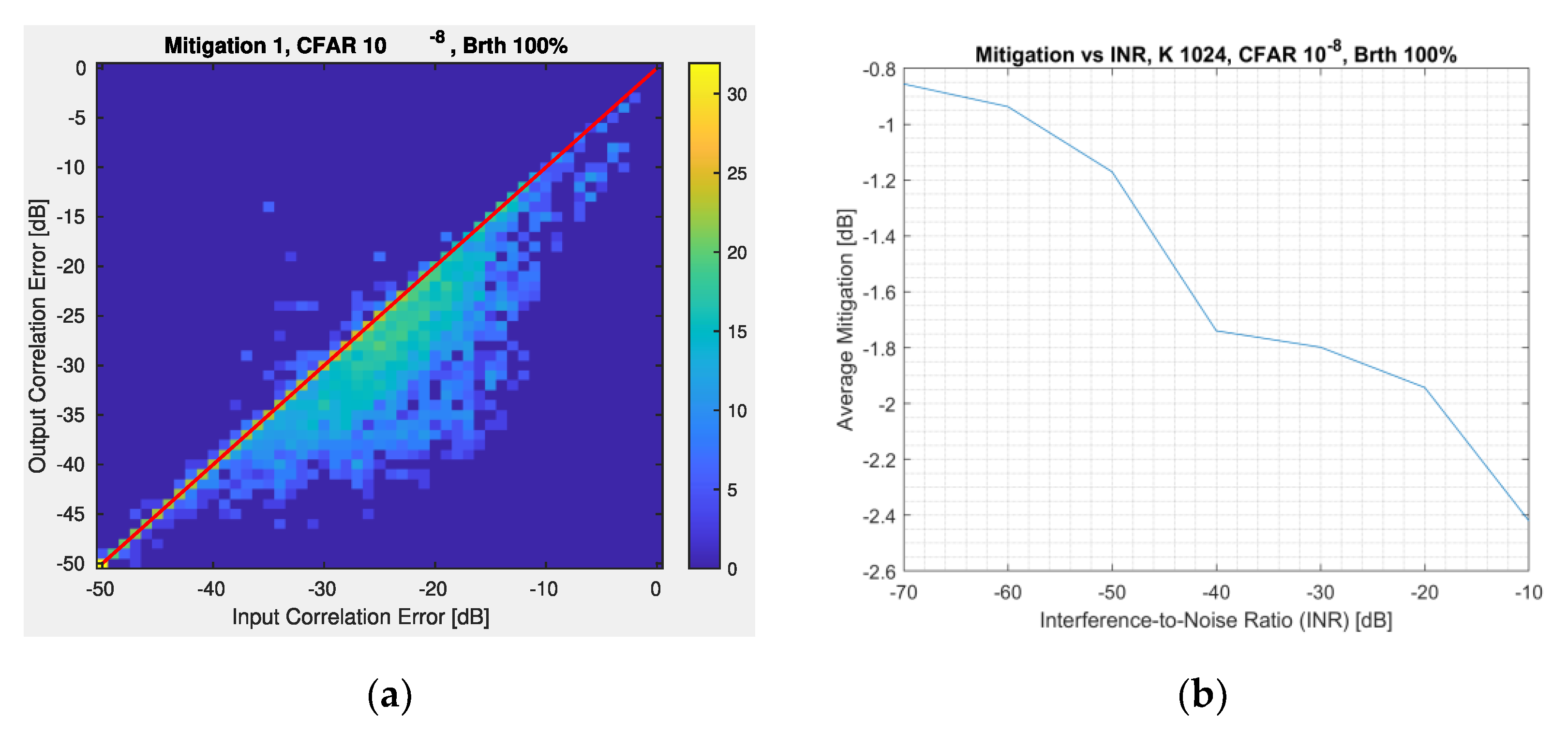
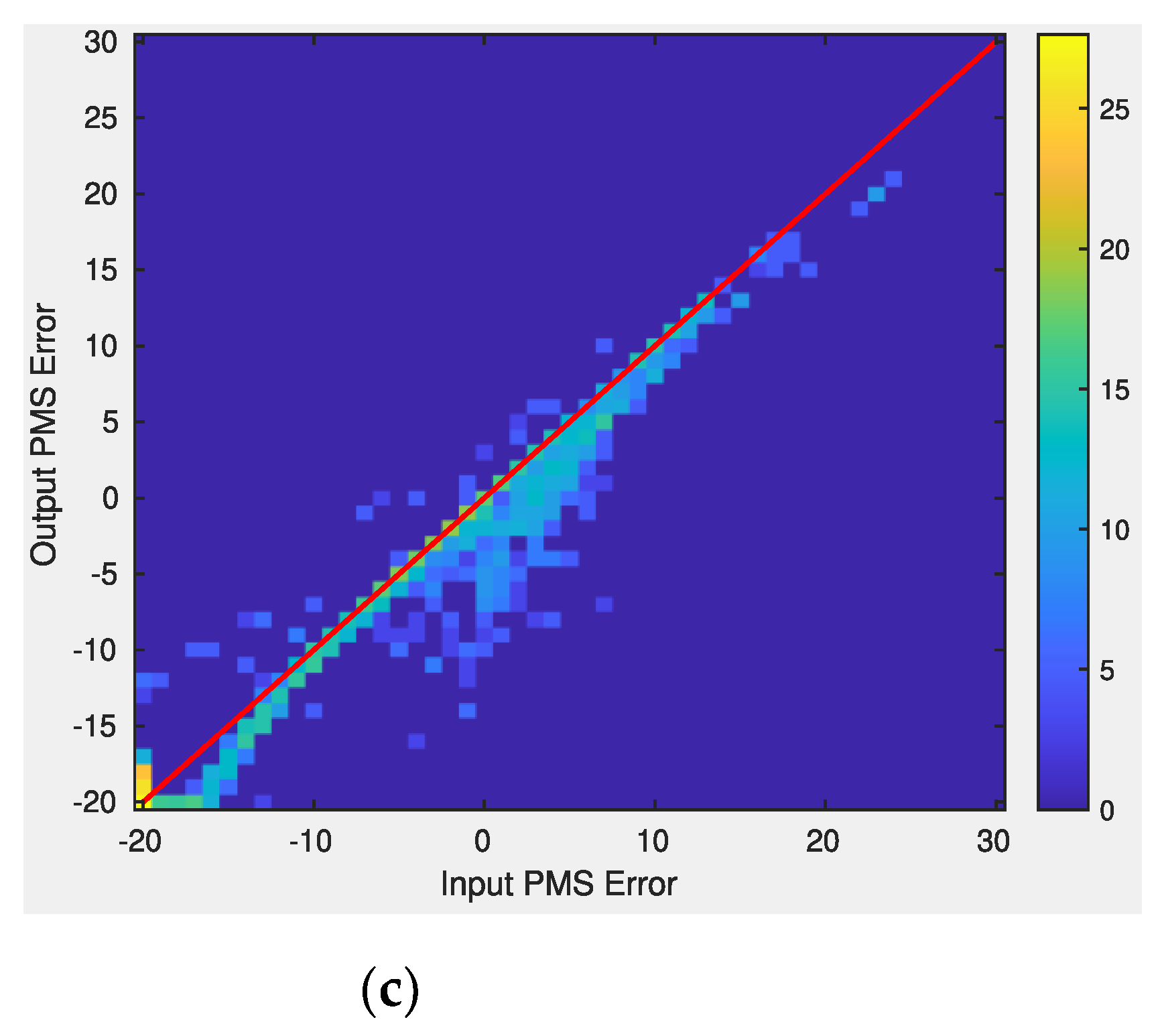
• K = 1024, no significant improvement was found for larger Ks except a better P_D (from 63 to 73%), at the expense of more hardware resources to compute the FFTs.
• CFAR = 10⁻⁸, with no significant variation up to 10⁻⁶, with a moderate P_D, and a negligible PFA (not detectable with the number of realizations performed). This offers less radiometric degradation and no big impact on mitigation.
• β_th = 100%, no significant impact down to 95%, but 100% offers the best mitigation vs. degradation trade-off.

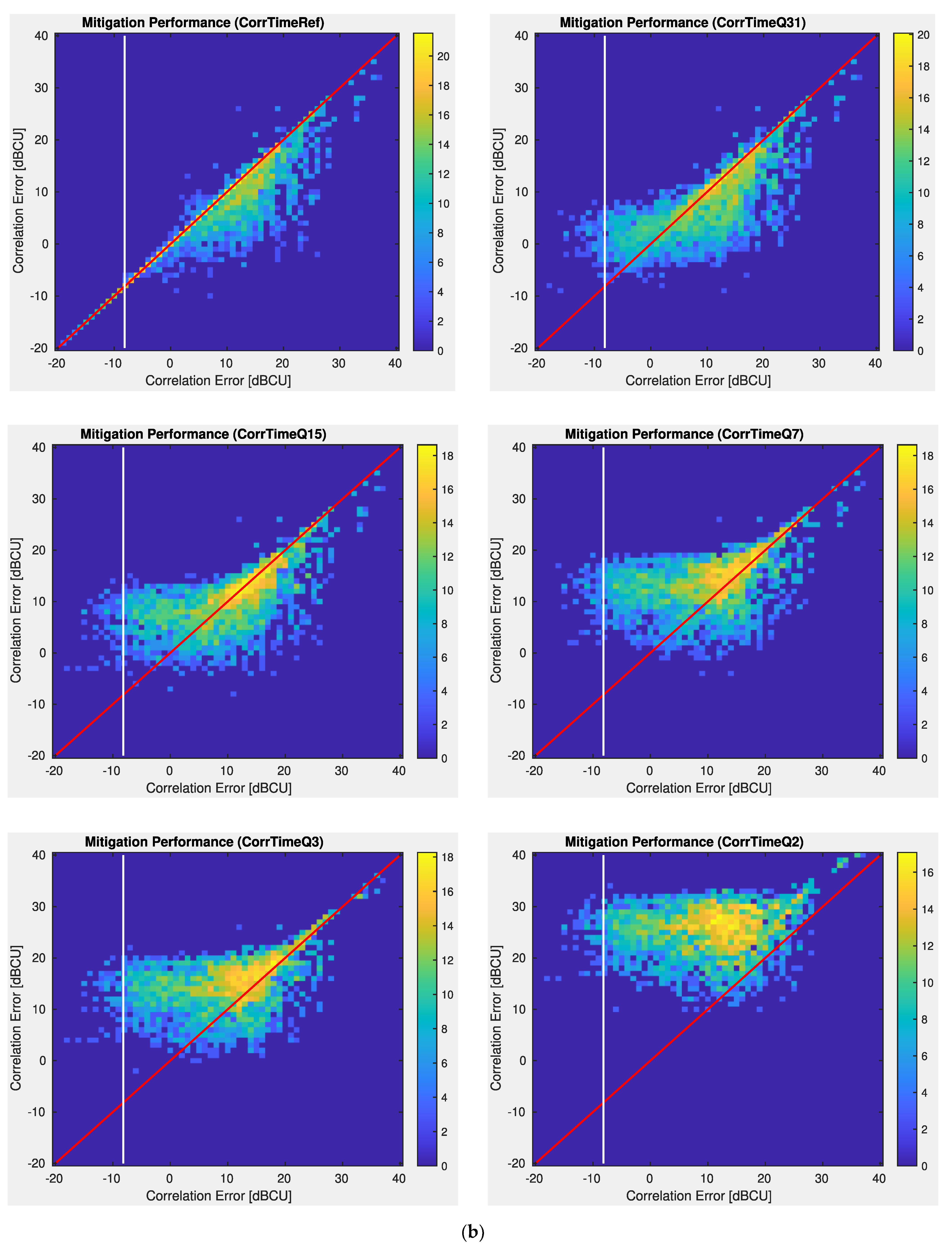
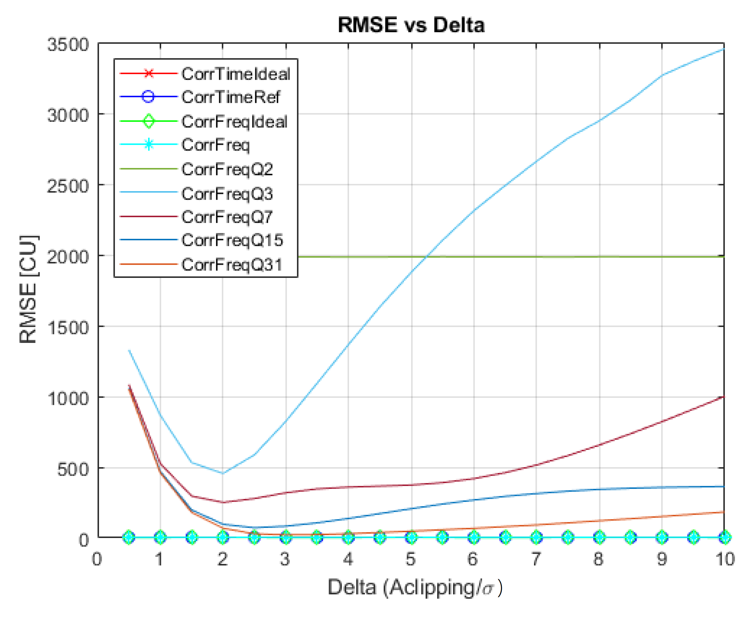
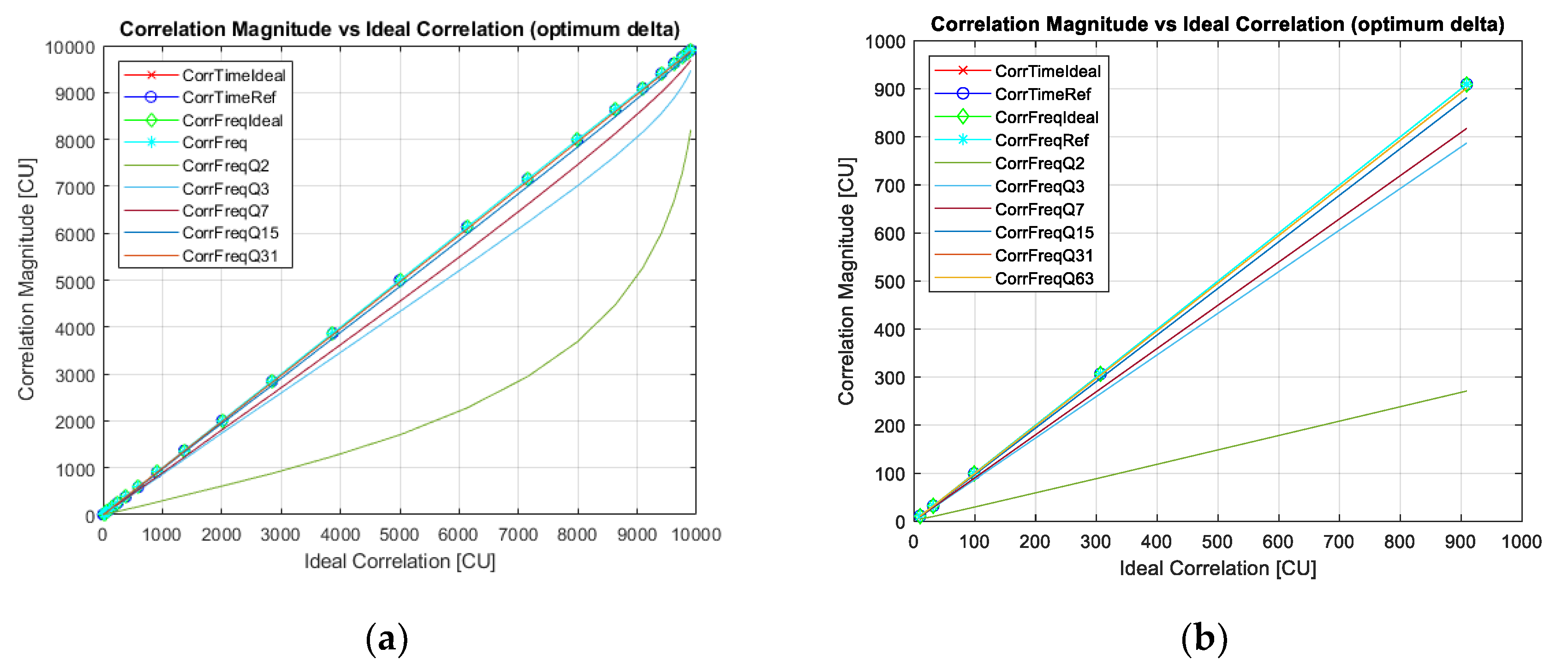
The RFI mitigation results are summarized in Figure 8, for both the cross-correlations and the PMS output.

4. Discussion

In the previous sections, the calculation of the Stokes parameters per frequency bin in the Short Time Fourier Transform (STFT) and the Polarimetric Kurtosis were introduced as key steps towards an efficient RFI detection and mitigation algorithm in Synthetic Aperture Interferometric Radiometers, using 1-bit quantization, as in for the planned SMOS follow-on missions.

After RFI mitigation, the signals are in the frequency domain; so, their complex correlation can be computed by transforming them back to either the time domain or the frequency domain, thanks to the Parseval’s theorem:

$${{\displaystyle \sum }}_{n=0}^{N-1}{x}_r\left[n\right]·y_r^{*}\left[n\right]={{\displaystyle \sum }}_{m=0}^{M-1}{{\displaystyle \sum }}_{k=0}^{K-1}{X}_r\left[m,k\right]·Y_r^{*}\left[m,k\right]$$

(27)

On the other hand, implementing the correlations with multipliers with a large number of bits is very resource-consuming. Two alternatives are discussed here:

• Quantize the signals in the frequency domain and perform the products with a reduced number of bits (1 to 5) so that multipliers can be more easily implemented using look-up tables (LUT).
• Transform the signals back to the time domain, quantize the signals in the time domain, and perform the products with a reduced number of bits (1 to 5).

Quantization introduces a non-linear effect between the ideal “analog” correlation and the one computed using quantized signals. These effects were introduced in [19], and analyzed more in-depth in [18]. However, for small correlation values the relationship is almost linear, and just a slope correction factor is required (1.0092 for 5 bits, 1.0321 for 4 bits, 1.1128 for 3 bits, 1.1558 for 2 bits, and 3.3670 for 1 bit), although it also amplifies the noise in the measurements (see Appendix A).

The simulation results for the frequency domain and time domain correlations with different numbers of bits are shown in Figure 9a,b. The vertical grey lines represent the 16-bit quantization noise floor: 10·log10(2⁻¹⁶) + 40 = −8.16 dBcu (1 cu = 10⁻⁴ = 1 correlator unit) as in SMOS. The horizontal lines represent the quantization noise floor for the different quantization levels. As can be appreciated, for a virtually infinite number of levels (top left scatter plot) there is no saturation effect. As the number of quantization bits (levels) decreases (5 to 1 bits: 31 to 2 levels) a saturation effect appears at the increasing levels: for 31 levels, the saturation occurs very close to the SMOS quantization noise floor and increases at ~+3 dB for every bit that is decreased. Note that the performance is significantly worse when the correlation is performed in the time domain due to the fact that the truncation to compute the FFTs already spreads the spectra, and the subsequent truncation degrades it even further.

The above results are summarized in

Table 7. Comparison results for the different correlator architectures under consideration. In green: optimum values.

Correlation Approach	All [1200 it.]		Mitigating (<0)		Degrading (>0)
FRef	Mean −3.00 dB	Std 4.22 dB	%. It. 57.5%	Mean −4.36 dB	%. It. 4.6%	Mean 1.82 dB
FQ31	Mean −3.28 dB	Std 4.25 dB	%. It. 65.9%	Mean −4.04 dB	%. It. 10.8%	Mean 1.00 dB
FQ15	Mean −3.37 dB	Std 4.28 dB	%. It. 65.6%	Mean −4.21 dB	%. It. 11.7%	Mean 1.14 dB
FQ7	Mean −3.35 dB	Std 4.35 dB	%. It. 64.1%	Mean −4.39 dB	%. It. 13.5%	Mean 1.49 dB
FQ3	Mean −2.73 dB	Std 4.45 dB	%. It. 59.9%	Mean −4.24 dB	%. It. 17.7%	Mean 2.33 dB
FQ2	Mean 0.06 dB	Std 5.27 dB	%. It. 40.1%	Mean −3.92 dB	%. It. 37.6%	Mean 4.32 dB
TRefIFFT	Mean −3.10 dB	Std 4.31 dB	%. It. 64.6%	Mean −3.85 dB	%. It. 12.3%	Mean 0.67 dB
TQ31	Mean −3.33 dB	Std 4.89 dB	%. It. 58.9%	Mean −4.88 dB	%. It. 18.9%	Mean 1.50 dB
TQ15	Mean −1.88 dB	Std 5.00 dB	%. It. 49.9%	Mean −4.34 dB	%. It. 27.9%	Mean 2.53 dB
TQ7	Mean 0.99 dB	Std 5.74 dB	%. It. 30.1%	Mean −4.34 dB	%. It. 47.8%	Mean 4.35 dB
TQ3	Mean 2.03 dB	Std 5.82 dB	%. It. 24.8%	Mean −4.13 dB	%. It. 53.0%	Mean 4.91 dB
TQ2	Mean 12.04 dB	Std 7.14 dB	%. It. 2.9%	Mean −3.28 dB	%. It. 74.9%	Mean 12.64 dB

showing that the performance of computing the cross-correlations in the frequency domain is much more efficient in terms of mitigation for 31, 15, and even 7 quantization levels, with actually very similar performances, and only approached by the cross-correlation in the time domain with 31 levels, although it mitigates in a smaller fraction of samples and degrades it in a larger fraction.

5. Conclusions

This study has presented a new RFI detection and mitigation algorithm for Synthetic Aperture Microwave Radiometers with coarse quantization schemes, such as the one planned for the SMOS follow-on mission. After signal windowing and channel equalization, statistical and polarimetric tests were applied in the time and/or frequency domains to detect the presence of RFI. As new features of this algorithm, it computes the Stokes parameters per frequency bin in the Short Time Fourier Transform (STFT) and also the so-called Polarimetric Kurtosis for the 3rd and 4th Stokes parameters. Finally, when RFI was detected in one of these domains or both, blanking masks were calculated and applied to remove the RFI.

For a CFAR of 10⁻⁸, it was found that the optimum parameters were: length of the FFTs equal to 1024 (without significant improvement found for larger values, except for a slightly better probability of detection: from 63 to 73%), β_th equal to 100% (i.e., only if the AND approach does not mitigate at all is the OR approach used), and application of Parseval’s theorem to compute the cross-correlations in the frequency domain using 31, 15, or even 7 quantization levels, with very similar performances among the three of them.

Finally, it is also worth mentioning that: (1) the algorithms presented can also be applied to (Polarimetric) Real Aperture Radiometers, despite R_avg = 1, and (2) the algorithm’ performance can be significantly improved if softer quantization schemes are used (i.e., more than 1 bit).

References

1. Gasiewski, A.; Klein, M.; Yevgrafov, A.; Leuskiy, V. Interference mitigation in passive microwave radiometry. In Proceedings of the IEEE International Geoscience and Remote Sensing Symposium, Toronto, ON, Canada, 24–28 June 2002; pp. 1682–1684. [Google Scholar]
2. Querol, J.; Onrubia, R.; Alonso-Arroyo, A.; Pascual, D.; Park, H.; Camps, A. Performance Assessment of Time–Frequency RFI Mitigation Techniques in Microwave Radiometry. IEEE J. Sel. Top. Appl. Earth Obs. Remote Sens. 2017, 10, 3096–3106. [Google Scholar] [CrossRef]
3. Erickson, A.; Rao, U. The Dimensions of RFI...and How ngVLA is Being Designed to Accommodate Them. Available online: https://www.ursi.org/proceedings/2019/rfi2019/24a3.pdf (accessed on 14 September 2022).
4. Querol, J.; Perez, A.; Camps, A. A Review of RFI Mitigation Techniques in Microwave Radiometry. Remote Sens. 2019, 11, 3042. [Google Scholar] [CrossRef]
5. Misra, S.; de Matthaeis, P. Passive Remote Sensing and Radio Frequency Interference (RFI): An Overview of Spectrum Allocations and RFI Management Algorithms [Technical Committees]. IEEE Geosci. Remote Sens. Mag. 2014, 2, 68–73. [Google Scholar] [CrossRef]
6. Landry, R.J.; Boutin, P.; Constantinescu, A. New anti-jamming technique for GPS and GALILEO receivers using adaptive FADP filter. Digit. Signal Process. A Rev. J. 2006, 16, 255–274. [Google Scholar] [CrossRef]
7. Tarongi, J.M.; Camps, A. Radio frequency interference detection and mitigation algorithms based on spectrogram analysis. Algorithms 2011, 4, 239–261. [Google Scholar] [CrossRef]
8. Antoni, J. The spectral kurtosis: A useful tool for characterizing non-stationary signals. Mech. Syst. Signal Process. 2006, 20, 282–307. [Google Scholar] [CrossRef]
9. Camps, A.; Tarongi, J.M. RFI Mitigation in Microwave Radiometry Using Wavelets. Algorithms 2009, 2, 1248–1262. [Google Scholar] [CrossRef]
10. Getu, T.M.; Ajib, W.; Landry, R. An Eigenvalue-Based Multi-Antenna RFI Detection Algorithm. In Proceedings of the 2018 IEEE 88th Vehicular Technology Conference (VTC-Fall), Chicago, IL, USA, 27–30 August 2018; pp. 1–5. [Google Scholar]
11. Nguyen, L.H.; Tran, T.D. A comprehensive performance comparison of RFI mitigation techniques for UWB radar signals. In Proceedings of the IEEE International Conference on Acoustics, Speech and Signal Processing (ICASSP), New Orleans, LA, USA, 5–9 March 2017; pp. 3086–3090. [Google Scholar]
12. Schoenwald, A.J.; Gholian, A.; Bradley, D.C.; Wong, M.; Mohammed, P.N.; Piepmeier, J.R. RFI detection and mitigation using independent component analysis as a pre-processor. In Proceedings of the 2016 Radio Frequency Interference (RFI), Socorro, NM, USA, 17–20 October 2016; pp. 100–104. [Google Scholar]
13. Díez-García, R.; Camps, A. A Novel RFI Detection Method for Microwave Radiometers Using Multilag Correlators. IEEE Trans. Geosci. Remote Sens. 2022, 60, 5300312. [Google Scholar] [CrossRef]
14. Camps, A.; Vall-llossera, M.; Duffo, N.; Zapata, M.; Corbella, I.; Torres, F.; Barrena, V. Sun effects in 2-D aperture synthesis radiometry imaging and their cancelation. IEEE Trans. Geosci. Remote Sens. 2004, 42, 1161–1167. [Google Scholar] [CrossRef]
15. Camps, A.; Park, H.; Gonzalez-Gambau, V. An imaging algorithm for synthetic aperture interferometric radiometers with built-in RFI mitigation. In Proceedings of the 2014 13th Specialist Meeting on Microwave Radiometry and Remote Sensing of the Environment (MicroRad), Pasadena, CA, USA, 24–27 March 2014; pp. 39–43. [Google Scholar] [CrossRef]
16. Camps, A.; Swift, C.T. New Techniques in Microwave Radiometry for Earth Remote Sensing: Principles and Applications. In Review of Radio Science, 1st ed.; Chapter 22; Wiley-IEEE Press: Hoboken, NJ, USA, 2002; ISBN 0471268666. [Google Scholar]
17. Emery, W.; Camps, A. Introduction to Satellite Remote Sensing; Elsevier: Amsterdam, The Netherlands, 2017. [Google Scholar] [CrossRef]
18. Bosch-Lluis, X.; Ramos-Perez, I.; Camps, A.; Rodriguez-Alvarez, N.; Valencia, E.; Park, H. A General Analysis of the Impact of Digitization in Microwave Correlation Radiometers. Sensors 2011, 11, 6066–6087. [Google Scholar] [CrossRef] [PubMed]
19. Hagen, J.; Farley, D. Digital-correlation techniques in radio science. Radio Sci. 1973, 8, 775–784. [Google Scholar] [CrossRef]
20. Camps, J.; Corbella, I.; Torres, F.; Bara, J.; Capdevila, J. RF interference analysis in aperture synthesis interferometric radiome-ters: Application to L-band MIRAS instrument. IEEE Trans. Geosci. Remote Sens. 2000, 38, 942–950. [Google Scholar] [CrossRef]
21. Camps, A.; Gourrion, J.; Tarongi, J.M.; Vall Llossera, M.; Gutierrez, A.; Barbosa, J.; Castro, R. Radio-Frequency Interference Detection and Mitigation Algorithms for Synthetic Aperture Radiometers. Algorithms 2011, 4, 155–182. [Google Scholar] [CrossRef]
22. González-Gambau, V.; Turiel, A.; Olmedo, E.; Martínez, J.; Corbella, I.; Camps, A. Nodal Sampling: A New Image Reconstruction Algorithm for SMOS. IEEE Trans. Geosci. Remote Sens. 2016, 54, 2314–2328. [Google Scholar] [CrossRef]
23. Van Vleck, J.H.; Middleton, D. The spectrum of clipped noise. Proc. IEEE 1966, 54, 2–19. [Google Scholar] [CrossRef]
24. Hall, M. Resolution and uncertainty in spectral decomposition. First Break 2006, 24, 43–47. [Google Scholar] [CrossRef]
25. Tarongi, J.M.; Camps, A. Normality Analysis for RFI Detection in Microwave Radiometry. Remote Sens. 2010, 2, 191–210. [Google Scholar] [CrossRef] [Green Version]
Figure 1. Characterization of the different RFI opportunities identified for present and future technologies. Modified from: “The Dimensions of RFI, and how ngVLA is Being Designed to Accommodate Them”, RFI 2019 [3].
Remotesensing 14 04672 g001
Figure 2. Overall block diagram of the proposed RFI mitigation algorithm.
Remotesensing 14 04672 g002
Figure 3. Modulus square of the STFT of the X-pol. at a sample receiver (a) before and (b) after equalization. The vertical lines appearing in both figures are due to the clipping of the input receiver signal due to the strong RFI signal.
Remotesensing 14 04672 g003
Figure 4. PDF (left) and CDF (right) of 2012 (yellow) and 2020 (orange) SMOS RFI observations. The simulated PDF and CDF is in blue.
Remotesensing 14 04672 g004
Figure 5. Multi-receiver kurtosis variance reduction as a function of the number of receivers averaged (Ravg) and SNR for a (a) multi-bit and (b) 1-bit quantization. SNR is the power relation between the correlated divided by the uncorrelated noise power.
Remotesensing 14 04672 g005
Figure 6. Probability of detection (PD) as a function of the INR, parameterized as a function of the variance reduction factor (ε), for (a) multi-bit, and (b) 1-bit quantization.
Remotesensing 14 04672 g006
Figure 7. Sensitivity improvement of the RFI detection [dB] as a function of the number of receivers averaged (Ravg) for the multi-bit and 1-bit quantization approaches.
Remotesensing 14 04672 g007
Figure 8. (a) Detection regimes after applying the algorithm; (b) average mitigation [dB] wrt. input INR [dB]; (c) input–output PMS error for CFAR = 10−8 and βth = 100%.
Remotesensing 14 04672 g008aRemotesensing 14 04672 g008b
Figure 9. Mitigation performance in the (a) frequency and (b) time domains as a function of the quantization levels: 2, 3, 7, 15, and 31 and multi-bit reference case (top left).
Remotesensing 14 04672 g009aRemotesensing 14 04672 g009b