


Changes over the Last 35 Years in Alaska’s Glaciated Landscape: A Novel Deep Learning Approach to Mapping Glaciers at Fine Temporal Granularity


Abstract
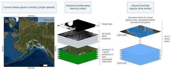
1. Introduction
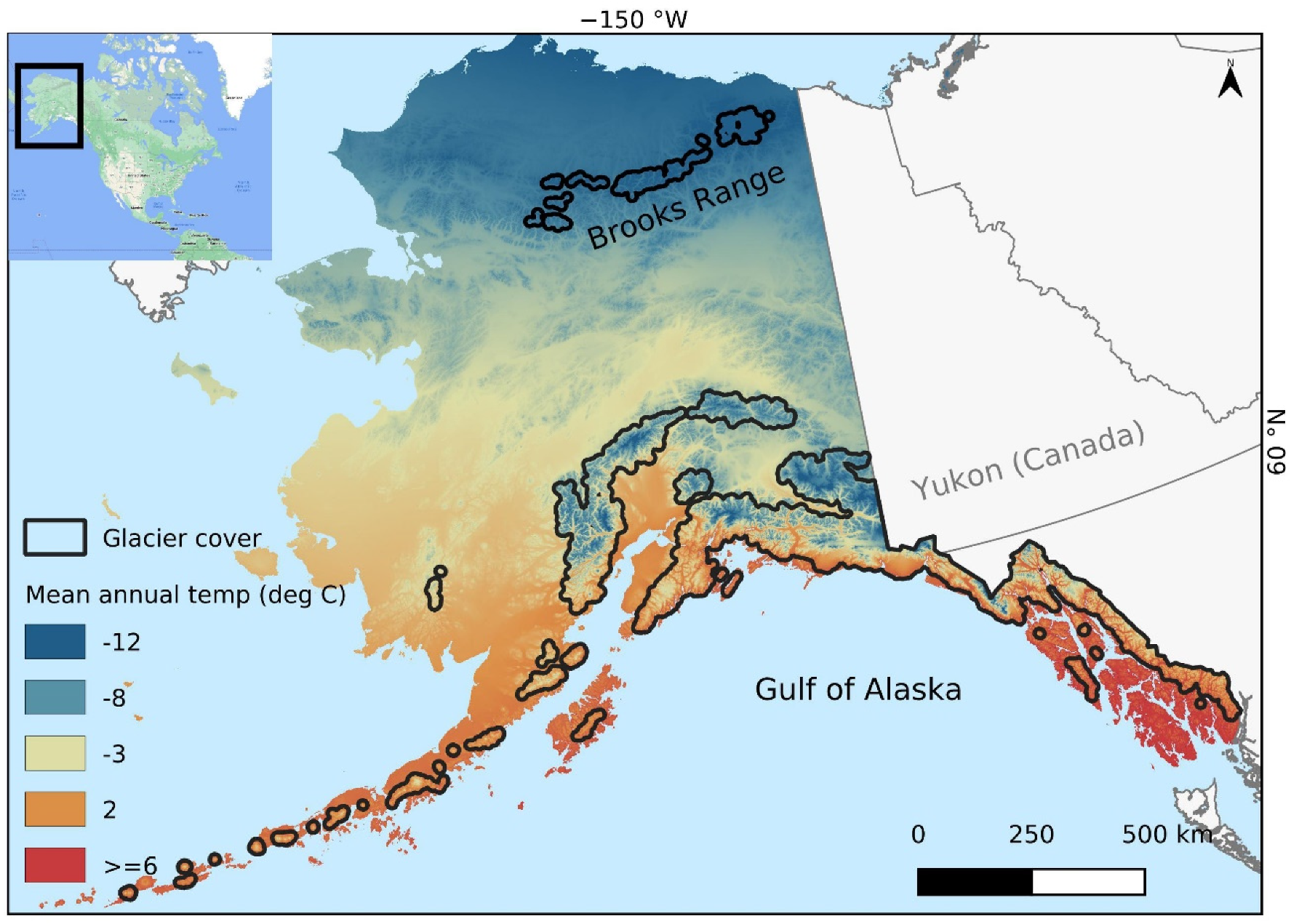
Study Area
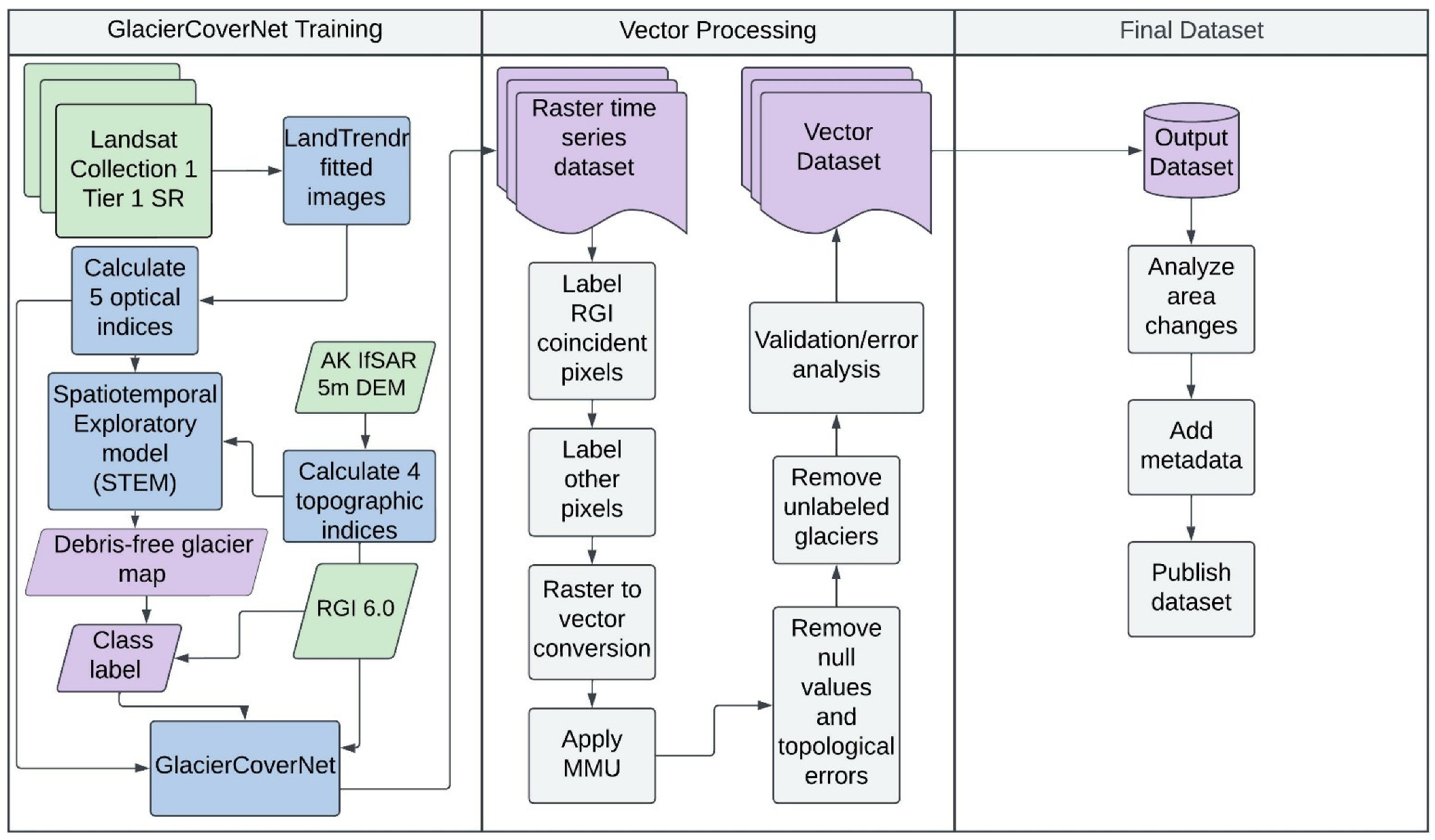
2. Materials and Methods
2.1. Landsat Archive and LandTrendr
2.2. Predictor Variables
2.3. Glacier Semantic Segmentation Dataset
2.3.1. Class Label Generation
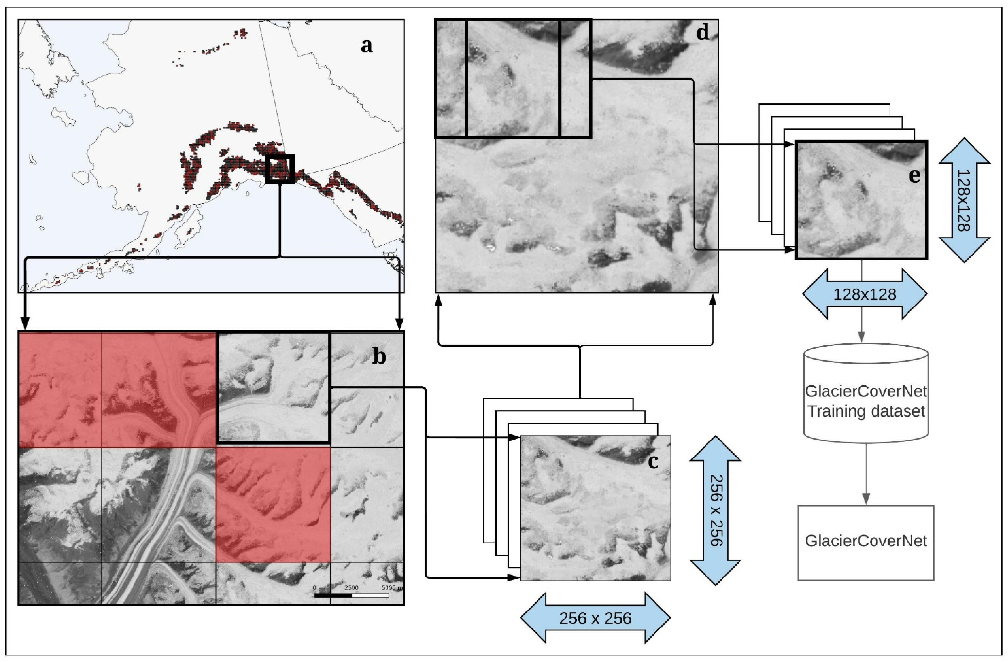
2.3.2. Training Data Generation
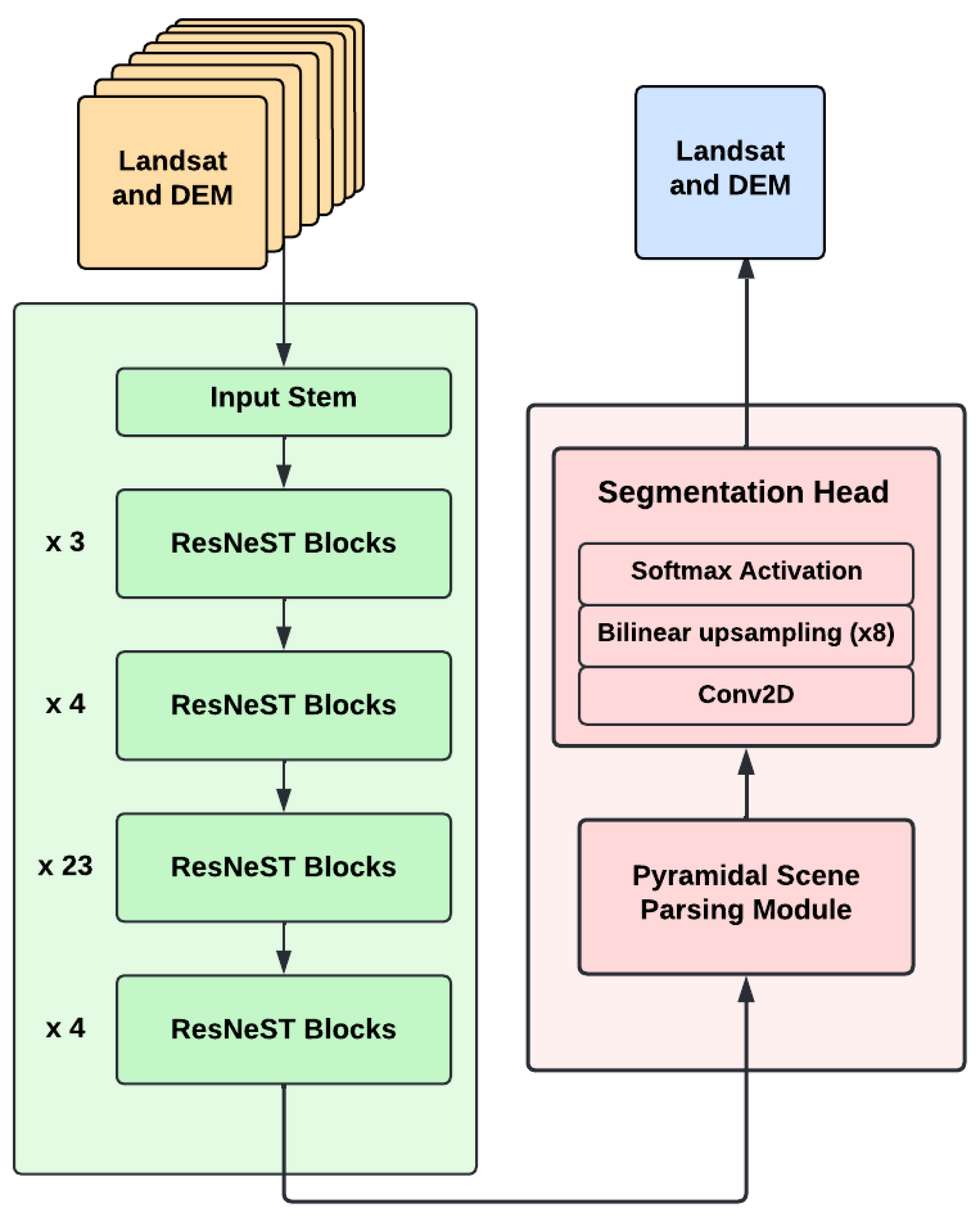
2.4. GlacierCoverNet Architecture
Encoder–Decoder Structure
2.5. Post-Processing Steps
2.6. Glacier Cover Change
2.7. Error Analysis Reference Datasets
3. Results
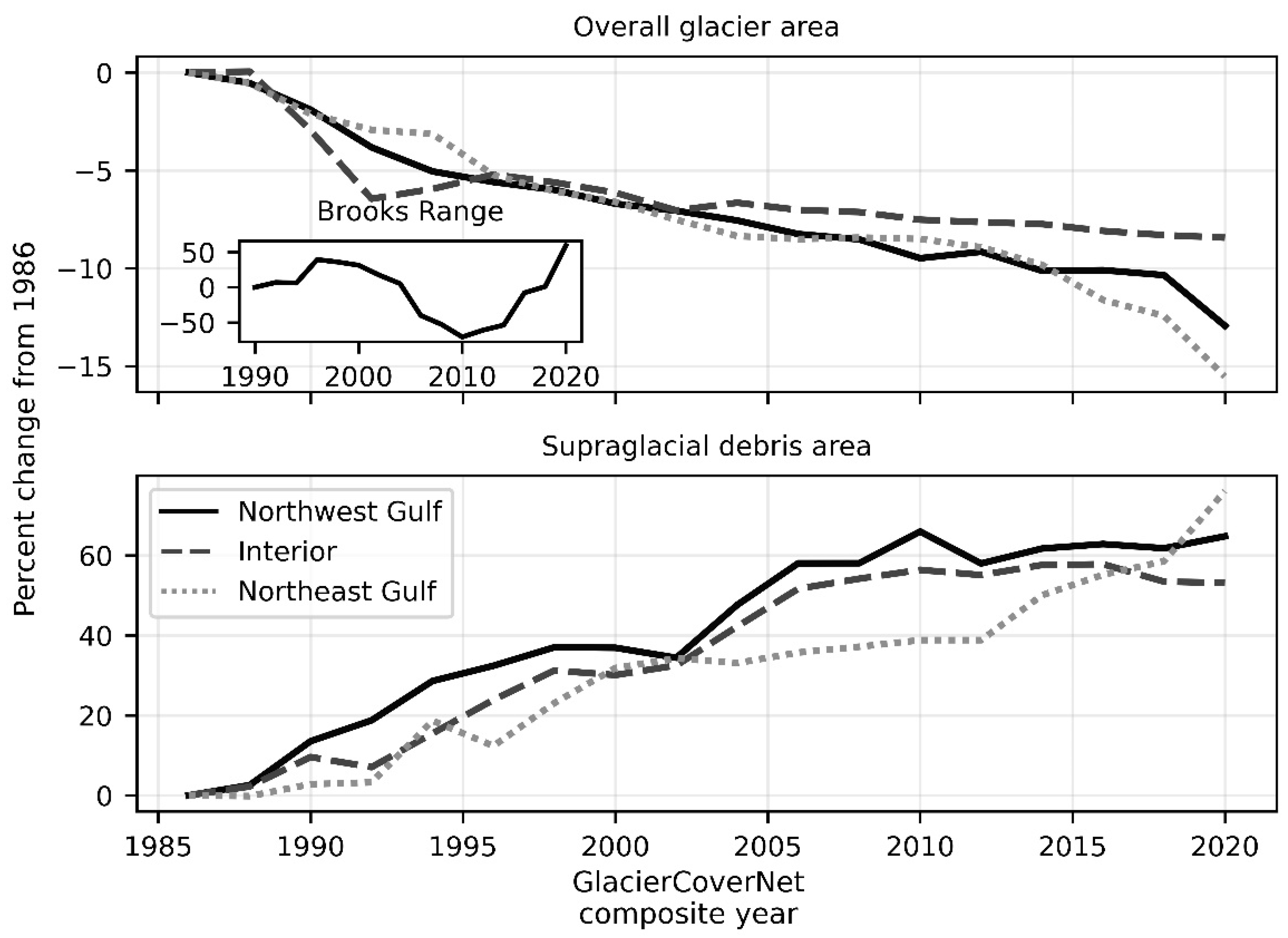
3.1. Areal Change over Time
3.1.1. Overall Glacier-Covered Area
3.1.2. Supraglacial Debris
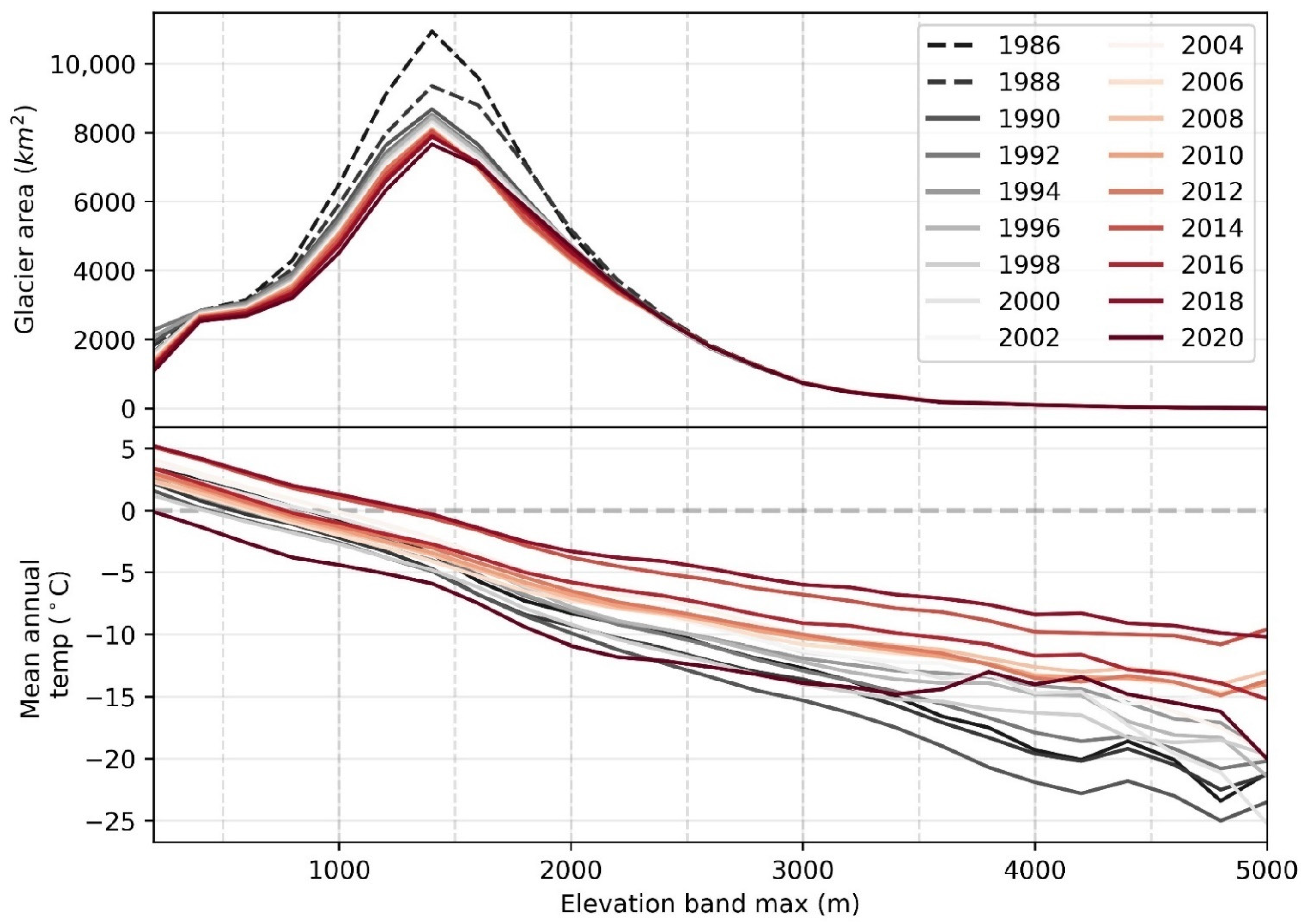
3.1.3. Changes with Elevation and Temperature
3.2. Error Analysis
3.2.1. Overall Glacier-Covered Area
3.2.2. Supraglacial Debris Error Analysis
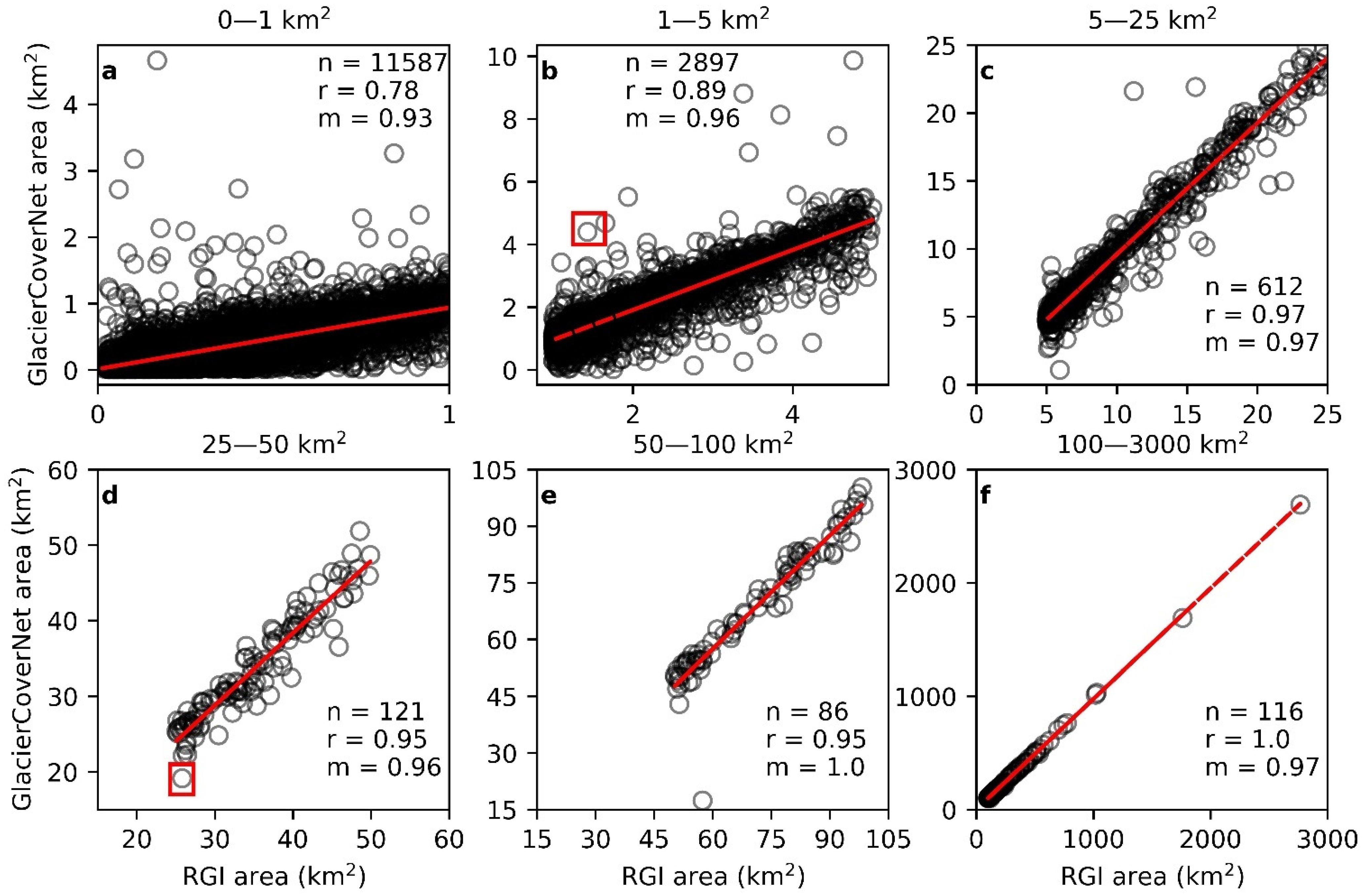
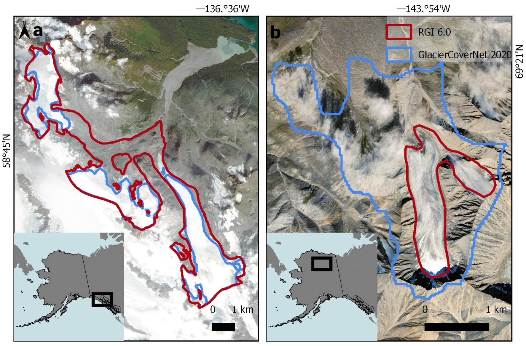
3.2.3. GlacierCoverNet vs. RGI for Individual Glaciers
4. Discussion
4.1. Status and Trends of Glacier-Covered Area
4.2. GlacierCoverNet Performance
4.3. Uncertainties and Future Work
5. Conclusions
Author Contributions
Funding
Data Availability Statement
Acknowledgments
Conflicts of Interest
Software Statement
Appendix A
Appendix A.1. GlacierCoverNet Architecture

Appendix A.2. Glacier-Covered Area Values

| Composite Year | Northwest Gulf | Northeast Gulf | Interior | Brooks Range | Total |
|---|---|---|---|---|---|
| 1986 | 15,625.1 | 32,648.3 | 15,803.5 | - | 64,076.9 |
| 1988 | 15,541.4 | 32,469.7 | 15,811.6 | - | |
| 1990 | 15,328.9 | 31,957.7 | 15,337.2 | 565.7 | |
| 1992 | 15,028.4 | 31,692.7 | 14,784.8 | 604.3 | |
| 1994 | 14,836.1 | 31,624.9 | 14,864.2 | 600.2 | |
| 1996 | 14,751.5 | 30,938.5 | 14,980.2 | 788.0 | |
| 1998 | 14,689.0 | 30,670.4 | 14,917.1 | 768.4 | |
| 2000 | 14,578.4 | 30,491.0 | 14,833.7 | 742.8 | |
| 2002 | 14,522.0 | 30,194.1 | 14,690.7 | 663.1 | |
| 2004 | 14,444.4 | 29,921.9 | 14,752.8 | 594.8 | |
| 2006 | 14,336.5 | 29,870.9 | 14,694.7 | 339.1 | |
| 2008 | 14,293.6 | 29,896.6 | 14,677.3 | 267.1 | |
| 2010 | 14,143.4 | 29,874.1 | 14,615.7 | 166.2 | |
| 2012 | 14,195.0 | 29,735.5 | 14,596.1 | 220.9 | |
| 2014 | 14,042.8 | 29,442.0 | 14,580.4 | 262.0 | |
| 2016 | 14,048.0 | 28,856.5 | 14,525.3 | 520.9 | |
| 2018 | 14,008.4 | 28,591.5 | 14,491.4 | 571.4 | |
| 2020 | 13,604.1 | 27,577.2 | 14,470.9 | 901.5 | 55,652.2 |
| Net Area Change | −2021.0 | −5071.1 | −1332.6 | 335.9 | −8424.7 |
| % Change | −12.9 | −15.5 | −8.4 | 59.4 | −13.1 |
| Composite Year | Northwest Gulf | Northeast Gulf | Interior | Total |
|---|---|---|---|---|
| 1986 | 1195.1 | 1560.5 | 1701.8 | 4457.3 |
| 1988 | 1225.7 | 1557.7 | 1739.7 | |
| 1990 | 1356.9 | 1604.1 | 1865.0 | |
| 1992 | 1419.2 | 1611.2 | 1821.9 | |
| 1994 | 1536.8 | 1851.9 | 1965.3 | |
| 1996 | 1582.3 | 1753.4 | 2108.2 | |
| 1998 | 1637.4 | 1920.7 | 2233.2 | |
| 2000 | 1636.0 | 2057.1 | 2213.7 | |
| 2002 | 1606.1 | 2095.0 | 2254.6 | |
| 2004 | 1764.1 | 2076.7 | 2420.2 | |
| 2006 | 1888.4 | 2117.7 | 2580.7 | |
| 2008 | 1888.5 | 2140.2 | 2623.4 | |
| 2010 | 1983.1 | 2166.0 | 2660.9 | |
| 2012 | 1887.8 | 2166.0 | 2638.9 | |
| 2014 | 1932.4 | 2341.2 | 2682.0 | |
| 2016 | 1945.7 | 2420.9 | 2685.0 | |
| 2018 | 1933.2 | 2473.5 | 2611.0 | |
| 2020 | 1969.0 | 2747.3 | 2606.1 | 7322.4 |
| Net area change | 773.9 | 1186.9 | 904.2 | 2865.0 |
| % Change | 64.8 | 76.1 | 53.1 | 64.3 |
Appendix A.3. Change in Glacier-Covered Area with Mean Annual Temperature and Elevation
| Year | Elevation Band (m) | Area (km2) | Mean Annual Temp (°C) | Standard Deviation |
|---|---|---|---|---|
| 1986 | 200 | 1617 | 3.6 | 1.0 |
| 1986 | 400 | 2836 | 2.4 | 1.1 |
| 1986 | 600 | 3155 | 1.4 | 1.4 |
| 1986 | 800 | 4308 | 0.3 | 1.8 |
| 1986 | 1000 | 6510 | −0.7 | 2.2 |
| 1986 | 1200 | 9108 | −1.9 | 2.6 |
| 1986 | 1400 | 10,936 | −3.5 | 3.3 |
| 1986 | 1600 | 9595 | −5.7 | 3.9 |
| 1986 | 1800 | 7159 | −7.3 | 3.9 |
| 1986 | 2000 | 5066 | −8.3 | 3.7 |
| 1986 | 2200 | 3551 | −9.1 | 3.1 |
| 1986 | 2400 | 2574 | −9.7 | 2.5 |
| 1986 | 2600 | 1764 | −10.9 | 2.2 |
| 1986 | 2800 | 1215 | −11.9 | 2.3 |
| 1986 | 3000 | 735 | −12.7 | 2.6 |
| 1986 | 3200 | 473 | −13.7 | 2.8 |
| 1986 | 3400 | 343 | −15.0 | 3.0 |
| 1986 | 3600 | 183 | −16.6 | 2.8 |
| 1986 | 3800 | 151 | −17.5 | 3.3 |
| 1986 | 4000 | 104 | −19.3 | 3.4 |
| 1986 | 4200 | 79 | −20.1 | 3.8 |
| 1986 | 4400 | 47 | −18.6 | 2.8 |
| 1986 | 4600 | 28 | −20.1 | 3.6 |
| 1986 | 4800 | 19 | −23.4 | 2.3 |
| 1986 | 5000 | 7 | −21.2 | 3.4 |
| 1988 | 200 | 1822 | 2.2 | 1.0 |
| 1988 | 400 | 2819 | 0.8 | 1.2 |
| 1988 | 600 | 3097 | −0.3 | 1.5 |
| 1988 | 800 | 4055 | −1.1 | 1.8 |
| 1988 | 1000 | 5932 | −2.2 | 2.0 |
| 1988 | 1200 | 7968 | −3.3 | 2.3 |
| 1988 | 1400 | 9351 | −4.7 | 3.0 |
| 1988 | 1600 | 8800 | −6.8 | 3.5 |
| 1988 | 1800 | 7083 | −8.4 | 3.2 |
| 1988 | 2000 | 5184 | −9.3 | 2.8 |
| 1988 | 2200 | 3731 | −10.3 | 2.2 |
| 1988 | 2400 | 2697 | −11.1 | 1.7 |
| 1988 | 2600 | 1837 | −12.1 | 1.6 |
| 1988 | 2800 | 1262 | −13.0 | 1.6 |
| 1988 | 3000 | 754 | −13.6 | 1.8 |
| 1988 | 3200 | 492 | −14.5 | 1.9 |
| 1988 | 3400 | 351 | −15.7 | 2.1 |
| 1988 | 3600 | 185 | −17.1 | 2.0 |
| 1988 | 3800 | 154 | −18.3 | 2.1 |
| 1988 | 4000 | 104 | −19.6 | 2.3 |
| 1988 | 4200 | 79 | −20.2 | 2.4 |
| 1988 | 4400 | 47 | −19.2 | 1.9 |
| 1988 | 4600 | 28 | −20.5 | 1.8 |
| 1988 | 4800 | 19 | −22.5 | 1.8 |
| 1988 | 5000 | 7 | −21.3 | 0.8 |
| 1990 | 200 | 1931 | 1.6 | 1.0 |
| 1990 | 400 | 2828 | 0.2 | 1.2 |
| 1990 | 600 | 3080 | −0.8 | 1.5 |
| 1990 | 800 | 3930 | −1.7 | 1.9 |
| 1990 | 1000 | 5609 | −2.6 | 2.2 |
| 1990 | 1200 | 7631 | −3.8 | 2.4 |
| 1990 | 1400 | 8684 | −4.9 | 2.5 |
| 1990 | 1600 | 7657 | −6.8 | 2.7 |
| 1990 | 1800 | 6132 | −8.5 | 2.5 |
| 1990 | 2000 | 4712 | −9.9 | 2.3 |
| 1990 | 2200 | 3568 | −11.2 | 2.0 |
| 1990 | 2400 | 2641 | −12.3 | 1.9 |
| 1990 | 2600 | 1808 | −13.4 | 2.1 |
| 1990 | 2800 | 1249 | −14.5 | 2.1 |
| 1990 | 3000 | 760 | −15.3 | 2.2 |
| 1990 | 3200 | 490 | −16.3 | 2.1 |
| 1990 | 3400 | 354 | −17.5 | 2.4 |
| 1990 | 3600 | 186 | −19.0 | 2.4 |
| 1990 | 3800 | 153 | −20.7 | 2.2 |
| 1990 | 4000 | 104 | −21.9 | 2.4 |
| 1990 | 4200 | 77 | −22.8 | 2.5 |
| 1990 | 4400 | 47 | −21.8 | 2.2 |
| 1990 | 4600 | 28 | −23.0 | 2.2 |
| 1990 | 4800 | 18 | −25.0 | 2.6 |
| 1990 | 5000 | 7 | −23.5 | 0.9 |
| 1992 | 200 | 2280 | 3.0 | 0.9 |
| 1992 | 400 | 2834 | 1.6 | 1.0 |
| 1992 | 600 | 3074 | 0.5 | 1.3 |
| 1992 | 800 | 3919 | −0.4 | 1.7 |
| 1992 | 1000 | 5484 | −1.3 | 1.9 |
| 1992 | 1200 | 7411 | −2.4 | 2.1 |
| 1992 | 1400 | 8523 | −3.5 | 2.4 |
| 1992 | 1600 | 7476 | −5.2 | 2.6 |
| 1992 | 1800 | 5995 | −6.9 | 2.6 |
| 1992 | 2000 | 4623 | −8.1 | 2.3 |
| 1992 | 2200 | 3436 | −9.2 | 2.0 |
| 1992 | 2400 | 2525 | −10.0 | 1.6 |
| 1992 | 2600 | 1741 | −10.9 | 1.5 |
| 1992 | 2800 | 1198 | −12.0 | 1.5 |
| 1992 | 3000 | 729 | −12.9 | 1.5 |
| 1992 | 3200 | 475 | −13.7 | 1.4 |
| 1992 | 3400 | 347 | −14.6 | 1.6 |
| 1992 | 3600 | 180 | −15.6 | 1.5 |
| 1992 | 3800 | 150 | −16.7 | 1.6 |
| 1992 | 4000 | 104 | −17.9 | 1.8 |
| 1992 | 4200 | 76 | −18.6 | 1.7 |
| 1992 | 4400 | 45 | −18.2 | 1.9 |
| 1992 | 4600 | 28 | −19.2 | 1.5 |
| 1992 | 4800 | 18 | −20.8 | 2.1 |
| 1992 | 5000 | 7 | −20.2 | 1.4 |
| 1994 | 200 | 2083 | 2.6 | 1.0 |
| 1994 | 400 | 2817 | 1.1 | 1.2 |
| 1994 | 600 | 3028 | 0.0 | 1.4 |
| 1994 | 800 | 3822 | −1.0 | 1.6 |
| 1994 | 1000 | 5368 | −2.0 | 1.6 |
| 1994 | 1200 | 7311 | −3.0 | 1.9 |
| 1994 | 1400 | 8490 | −4.0 | 2.1 |
| 1994 | 1600 | 7418 | −5.3 | 2.4 |
| 1994 | 1800 | 5981 | −6.8 | 2.4 |
| 1994 | 2000 | 4643 | −8.1 | 2.1 |
| 1994 | 2200 | 3439 | −9.0 | 1.8 |
| 1994 | 2400 | 2539 | −9.6 | 1.6 |
| 1994 | 2600 | 1746 | −10.3 | 1.7 |
| 1994 | 2800 | 1233 | −11.1 | 2.0 |
| 1994 | 3000 | 745 | −11.9 | 2.0 |
| 1994 | 3200 | 486 | −12.4 | 2.1 |
| 1994 | 3400 | 348 | −12.9 | 2.1 |
| 1994 | 3600 | 181 | −13.1 | 2.2 |
| 1994 | 3800 | 152 | −13.4 | 2.2 |
| 1994 | 4000 | 104 | −14.1 | 2.3 |
| 1994 | 4200 | 78 | −14.4 | 2.3 |
| 1994 | 4400 | 47 | −15.5 | 1.8 |
| 1994 | 4600 | 28 | −16.8 | 2.1 |
| 1994 | 4800 | 19 | −17.1 | 2.2 |
| 1994 | 5000 | 7 | −19.7 | 1.1 |
| 1996 | 200 | 1602 | 3.1 | 1.1 |
| 1996 | 400 | 2790 | 1.9 | 1.3 |
| 1996 | 600 | 2971 | 0.7 | 1.5 |
| 1996 | 800 | 3740 | −0.2 | 1.9 |
| 1996 | 1000 | 5316 | −1.1 | 2.1 |
| 1996 | 1200 | 7272 | −2.1 | 2.3 |
| 1996 | 1400 | 8431 | −3.0 | 2.5 |
| 1996 | 1600 | 7425 | −4.5 | 2.9 |
| 1996 | 1800 | 6042 | −6.2 | 3.1 |
| 1996 | 2000 | 4741 | −7.8 | 3.0 |
| 1996 | 2200 | 3510 | −8.9 | 2.6 |
| 1996 | 2400 | 2569 | −9.6 | 1.9 |
| 1996 | 2600 | 1786 | −10.4 | 1.7 |
| 1996 | 2800 | 1240 | −11.3 | 1.8 |
| 1996 | 3000 | 753 | −12.2 | 1.9 |
| 1996 | 3200 | 487 | −13.0 | 2.0 |
| 1996 | 3400 | 343 | −13.6 | 2.2 |
| 1996 | 3600 | 182 | −13.9 | 2.5 |
| 1996 | 3800 | 150 | −13.9 | 2.3 |
| 1996 | 4000 | 104 | −14.8 | 2.8 |
| 1996 | 4200 | 78 | −14.9 | 2.8 |
| 1996 | 4400 | 48 | −17.0 | 2.4 |
| 1996 | 4600 | 28 | −18.1 | 2.7 |
| 1996 | 4800 | 19 | −18.3 | 3.5 |
| 1996 | 5000 | 7 | −21.4 | 2.3 |
| 1998 | 200 | 1599 | 1.2 | 1.2 |
| 1998 | 400 | 2766 | 0.1 | 1.3 |
| 1998 | 600 | 2941 | −0.9 | 1.5 |
| 1998 | 800 | 3696 | −1.8 | 1.8 |
| 1998 | 1000 | 5284 | −2.7 | 1.9 |
| 1998 | 1200 | 7155 | −3.8 | 2.2 |
| 1998 | 1400 | 8324 | −4.8 | 2.3 |
| 1998 | 1600 | 7307 | −6.2 | 2.3 |
| 1998 | 1800 | 5965 | −7.9 | 2.1 |
| 1998 | 2000 | 4703 | −9.2 | 1.9 |
| 1998 | 2200 | 3489 | −10.4 | 1.6 |
| 1998 | 2400 | 2564 | −11.3 | 1.7 |
| 1998 | 2600 | 1777 | −12.2 | 1.8 |
| 1998 | 2800 | 1230 | −13.2 | 2.0 |
| 1998 | 3000 | 746 | −14.0 | 2.0 |
| 1998 | 3200 | 486 | −14.6 | 2.1 |
| 1998 | 3400 | 347 | −15.2 | 2.3 |
| 1998 | 3600 | 183 | −15.4 | 2.3 |
| 1998 | 3800 | 152 | −16.0 | 2.7 |
| 1998 | 4000 | 102 | −16.3 | 2.8 |
| 1998 | 4200 | 78 | −16.5 | 3.0 |
| 1998 | 4400 | 48 | −18.3 | 2.2 |
| 1998 | 4600 | 28 | −18.7 | 2.2 |
| 1998 | 4800 | 19 | −18.5 | 1.6 |
| 1998 | 5000 | 7 | −19.7 | 1.9 |
| 2000 | 200 | 1514 | 3.3 | 0.9 |
| 2000 | 400 | 2738 | 2.3 | 0.9 |
| 2000 | 600 | 2901 | 1.3 | 1.2 |
| 2000 | 800 | 3657 | 0.3 | 1.4 |
| 2000 | 1000 | 5218 | −0.6 | 1.4 |
| 2000 | 1200 | 7105 | −1.7 | 1.6 |
| 2000 | 1400 | 8283 | −2.9 | 1.9 |
| 2000 | 1600 | 7282 | −4.5 | 2.4 |
| 2000 | 1800 | 5933 | −6.1 | 2.9 |
| 2000 | 2000 | 4666 | −7.1 | 2.9 |
| 2000 | 2200 | 3469 | −7.6 | 2.6 |
| 2000 | 2400 | 2569 | −8.2 | 2.2 |
| 2000 | 2600 | 1794 | −9.2 | 2.4 |
| 2000 | 2800 | 1246 | −10.3 | 2.7 |
| 2000 | 3000 | 757 | −11.4 | 3.1 |
| 2000 | 3200 | 495 | −11.8 | 3.0 |
| 2000 | 3400 | 351 | −12.7 | 3.2 |
| 2000 | 3600 | 187 | −13.5 | 3.6 |
| 2000 | 3800 | 151 | −13.2 | 3.1 |
| 2000 | 4000 | 103 | −14.7 | 4.2 |
| 2000 | 4200 | 78 | −14.6 | 3.9 |
| 2000 | 4400 | 48 | −17.3 | 4.1 |
| 2000 | 4600 | 28 | −19.6 | 5.0 |
| 2000 | 4800 | 19 | −21.1 | 6.0 |
| 2000 | 5000 | 7 | −25.2 | 3.7 |
| 2002 | 200 | 1464 | 3.7 | 1.0 |
| 2002 | 400 | 2733 | 2.8 | 0.9 |
| 2002 | 600 | 2914 | 1.8 | 1.1 |
| 2002 | 800 | 3638 | 0.9 | 1.3 |
| 2002 | 1000 | 5175 | −0.1 | 1.4 |
| 2002 | 1200 | 7016 | −1.2 | 1.5 |
| 2002 | 1400 | 8207 | −2.2 | 1.7 |
| 2002 | 1600 | 7181 | −3.6 | 2.0 |
| 2002 | 1800 | 5857 | −5.2 | 2.4 |
| 2002 | 2000 | 4576 | −6.5 | 2.4 |
| 2002 | 2200 | 3422 | −7.6 | 2.3 |
| 2002 | 2400 | 2547 | −8.5 | 2.2 |
| 2002 | 2600 | 1784 | −9.4 | 2.4 |
| 2002 | 2800 | 1240 | −10.4 | 2.5 |
| 2002 | 3000 | 752 | −11.3 | 2.7 |
| 2002 | 3200 | 496 | −11.8 | 2.8 |
| 2002 | 3400 | 353 | −12.2 | 2.8 |
| 2002 | 3600 | 190 | −12.3 | 2.8 |
| 2002 | 3800 | 149 | −13.3 | 3.1 |
| 2002 | 4000 | 103 | −13.4 | 3.3 |
| 2002 | 4200 | 78 | −13.5 | 3.5 |
| 2002 | 4400 | 47 | −15.6 | 3.7 |
| 2002 | 4600 | 27 | −15.4 | 3.5 |
| 2002 | 4800 | 19 | −14.6 | 2.4 |
| 2002 | 5000 | 8 | −14.5 | 2.5 |
| 2004 | 200 | 1450 | 4.1 | 1.0 |
| 2004 | 400 | 2725 | 3.0 | 0.9 |
| 2004 | 600 | 2892 | 1.9 | 1.1 |
| 2004 | 800 | 3617 | 0.9 | 1.2 |
| 2004 | 1000 | 5096 | −0.1 | 1.3 |
| 2004 | 1200 | 6926 | −1.1 | 1.5 |
| 2004 | 1400 | 8141 | −2.2 | 1.6 |
| 2004 | 1600 | 7132 | −3.5 | 1.9 |
| 2004 | 1800 | 5762 | −4.9 | 2.2 |
| 2004 | 2000 | 4545 | −6.0 | 2.3 |
| 2004 | 2200 | 3426 | −6.8 | 2.1 |
| 2004 | 2400 | 2588 | −7.2 | 1.8 |
| 2004 | 2600 | 1797 | −8.1 | 1.8 |
| 2004 | 2800 | 1237 | −9.1 | 2.0 |
| 2004 | 3000 | 750 | −10.0 | 2.3 |
| 2004 | 3200 | 493 | −10.5 | 2.1 |
| 2004 | 3400 | 350 | −11.1 | 2.2 |
| 2004 | 3600 | 187 | −11.7 | 2.1 |
| 2004 | 3800 | 151 | −11.9 | 1.9 |
| 2004 | 4000 | 103 | −13.2 | 2.6 |
| 2004 | 4200 | 79 | −13.4 | 2.4 |
| 2004 | 4400 | 46 | −14.8 | 2.2 |
| 2004 | 4600 | 28 | −16.2 | 2.6 |
| 2004 | 4800 | 19 | −17.5 | 3.0 |
| 2004 | 5000 | 8 | −19.6 | 2.7 |
| 2006 | 200 | 1417 | 2.3 | 1.0 |
| 2006 | 400 | 2720 | 1.2 | 1.0 |
| 2006 | 600 | 2890 | 0.1 | 1.2 |
| 2006 | 800 | 3594 | −1.0 | 1.3 |
| 2006 | 1000 | 5090 | −2.0 | 1.4 |
| 2006 | 1200 | 6935 | −3.0 | 1.6 |
| 2006 | 1400 | 8116 | −4.1 | 1.8 |
| 2006 | 1600 | 7074 | −5.3 | 2.1 |
| 2006 | 1800 | 5605 | −6.5 | 2.3 |
| 2006 | 2000 | 4419 | −7.3 | 2.2 |
| 2006 | 2200 | 3376 | −7.9 | 1.9 |
| 2006 | 2400 | 2569 | −8.4 | 1.7 |
| 2006 | 2600 | 1791 | −9.2 | 1.7 |
| 2006 | 2800 | 1238 | −10.1 | 2.1 |
| 2006 | 3000 | 739 | −10.8 | 2.5 |
| 2006 | 3200 | 489 | −11.1 | 2.1 |
| 2006 | 3400 | 345 | −11.5 | 2.0 |
| 2006 | 3600 | 185 | −11.8 | 1.4 |
| 2006 | 3800 | 150 | −12.4 | 1.5 |
| 2006 | 4000 | 103 | −13.2 | 1.7 |
| 2006 | 4200 | 78 | −13.5 | 1.7 |
| 2006 | 4400 | 46 | −13.6 | 1.2 |
| 2006 | 4600 | 28 | −13.9 | 1.2 |
| 2006 | 4800 | 18 | −14.7 | 1.0 |
| 2006 | 5000 | 8 | −13.9 | 0.6 |
| 2008 | 200 | 1402 | 2.4 | 0.9 |
| 2008 | 400 | 2707 | 1.4 | 1.1 |
| 2008 | 600 | 2875 | 0.3 | 1.3 |
| 2008 | 800 | 3571 | −0.8 | 1.4 |
| 2008 | 1000 | 5098 | −1.7 | 1.6 |
| 2008 | 1200 | 6949 | −2.6 | 1.9 |
| 2008 | 1400 | 8103 | −3.6 | 2.0 |
| 2008 | 1600 | 7035 | −4.8 | 2.2 |
| 2008 | 1800 | 5511 | −6.0 | 2.3 |
| 2008 | 2000 | 4365 | −7.1 | 2.4 |
| 2008 | 2200 | 3380 | −7.9 | 2.4 |
| 2008 | 2400 | 2583 | −8.3 | 2.0 |
| 2008 | 2600 | 1804 | −8.9 | 1.8 |
| 2008 | 2800 | 1240 | −9.6 | 2.0 |
| 2008 | 3000 | 738 | −10.3 | 2.4 |
| 2008 | 3200 | 488 | −10.5 | 2.1 |
| 2008 | 3400 | 347 | −10.9 | 1.9 |
| 2008 | 3600 | 183 | −11.2 | 1.4 |
| 2008 | 3800 | 151 | −11.9 | 1.5 |
| 2008 | 4000 | 103 | −12.6 | 1.8 |
| 2008 | 4200 | 78 | −13.0 | 1.7 |
| 2008 | 4400 | 46 | −12.7 | 1.1 |
| 2008 | 4600 | 28 | −13.1 | 1.1 |
| 2008 | 4800 | 19 | −14.0 | 1.3 |
| 2008 | 5000 | 8 | −13.0 | 0.5 |
| 2010 | 200 | 1369 | 2.8 | 0.9 |
| 2010 | 400 | 2685 | 1.7 | 1.1 |
| 2010 | 600 | 2867 | 0.6 | 1.4 |
| 2010 | 800 | 3566 | −0.6 | 1.5 |
| 2010 | 1000 | 5084 | −1.5 | 1.7 |
| 2010 | 1200 | 6932 | −2.5 | 2.0 |
| 2010 | 1400 | 8097 | −3.4 | 2.3 |
| 2010 | 1600 | 6984 | −4.6 | 2.5 |
| 2010 | 1800 | 5429 | −5.8 | 2.4 |
| 2010 | 2000 | 4300 | −6.8 | 2.3 |
| 2010 | 2200 | 3350 | −7.7 | 2.2 |
| 2010 | 2400 | 2578 | −8.2 | 1.9 |
| 2010 | 2600 | 1802 | −8.9 | 1.7 |
| 2010 | 2800 | 1246 | −9.7 | 1.8 |
| 2010 | 3000 | 745 | −10.3 | 2.1 |
| 2010 | 3200 | 491 | −10.7 | 2.0 |
| 2010 | 3400 | 348 | −11.3 | 2.2 |
| 2010 | 3600 | 184 | −11.8 | 1.8 |
| 2010 | 3800 | 151 | −12.3 | 2.1 |
| 2010 | 4000 | 103 | −13.3 | 2.5 |
| 2010 | 4200 | 79 | −13.4 | 2.3 |
| 2010 | 4400 | 47 | −13.5 | 1.0 |
| 2010 | 4600 | 27 | −13.8 | 1.0 |
| 2010 | 4800 | 19 | −14.8 | 1.0 |
| 2010 | 5000 | 8 | −14.0 | 1.2 |
| 2012 | 200 | 1324 | 3.0 | 0.9 |
| 2012 | 400 | 2656 | 1.9 | 1.2 |
| 2012 | 600 | 2842 | 0.7 | 1.5 |
| 2012 | 800 | 3512 | −0.4 | 1.7 |
| 2012 | 1000 | 5021 | −1.3 | 1.9 |
| 2012 | 1200 | 6926 | −2.1 | 2.2 |
| 2012 | 1400 | 8066 | −3.0 | 2.5 |
| 2012 | 1600 | 6975 | −4.2 | 2.8 |
| 2012 | 1800 | 5467 | −5.4 | 2.7 |
| 2012 | 2000 | 4341 | −6.5 | 2.7 |
| 2012 | 2200 | 3389 | −7.4 | 2.7 |
| 2012 | 2400 | 2596 | −8.0 | 2.3 |
| 2012 | 2600 | 1808 | −8.7 | 2.0 |
| 2012 | 2800 | 1243 | −9.4 | 2.0 |
| 2012 | 3000 | 740 | −10.0 | 2.2 |
| 2012 | 3200 | 488 | −10.6 | 2.2 |
| 2012 | 3400 | 346 | −11.0 | 2.4 |
| 2012 | 3600 | 184 | −11.5 | 2.1 |
| 2012 | 3800 | 153 | −12.4 | 2.1 |
| 2012 | 4000 | 103 | −13.5 | 2.1 |
| 2012 | 4200 | 78 | −13.8 | 2.1 |
| 2012 | 4400 | 46 | −13.3 | 1.1 |
| 2012 | 4600 | 27 | −13.8 | 1.2 |
| 2012 | 4800 | 18 | −14.9 | 1.2 |
| 2012 | 5000 | 8 | −13.7 | 1.1 |
| 2014 | 200 | 1285 | 5.1 | 0.9 |
| 2014 | 400 | 2638 | 4.1 | 1.2 |
| 2014 | 600 | 2832 | 2.9 | 1.4 |
| 2014 | 800 | 3436 | 1.8 | 1.5 |
| 2014 | 1000 | 4906 | 1.0 | 1.6 |
| 2014 | 1200 | 6785 | 0.2 | 2.0 |
| 2014 | 1400 | 8039 | −0.6 | 2.4 |
| 2014 | 1600 | 7044 | −1.6 | 2.7 |
| 2014 | 1800 | 5535 | −2.8 | 2.7 |
| 2014 | 2000 | 4376 | −3.8 | 2.7 |
| 2014 | 2200 | 3390 | −4.5 | 2.7 |
| 2014 | 2400 | 2596 | −5.1 | 2.3 |
| 2014 | 2600 | 1809 | −5.6 | 2.0 |
| 2014 | 2800 | 1239 | −6.3 | 2.0 |
| 2014 | 3000 | 743 | −6.8 | 2.1 |
| 2014 | 3200 | 486 | −7.3 | 2.0 |
| 2014 | 3400 | 343 | −7.9 | 2.2 |
| 2014 | 3600 | 180 | −8.2 | 1.8 |
| 2014 | 3800 | 152 | −8.9 | 2.1 |
| 2014 | 4000 | 103 | −9.8 | 2.1 |
| 2014 | 4200 | 77 | −9.9 | 1.6 |
| 2014 | 4400 | 44 | −10.0 | 1.4 |
| 2014 | 4600 | 26 | −10.1 | 1.4 |
| 2014 | 4800 | 18 | −10.8 | 1.3 |
| 2014 | 5000 | 6 | −9.6 | 1.4 |
| 2016 | 200 | 1254 | 3.4 | 1.0 |
| 2016 | 400 | 2615 | 2.2 | 1.3 |
| 2016 | 600 | 2788 | 1.0 | 1.5 |
| 2016 | 800 | 3371 | −0.2 | 1.6 |
| 2016 | 1000 | 4786 | −1.0 | 1.7 |
| 2016 | 1200 | 6657 | −1.9 | 2.0 |
| 2016 | 1400 | 7925 | −2.7 | 2.3 |
| 2016 | 1600 | 7103 | −3.8 | 2.6 |
| 2016 | 1800 | 5690 | −5.0 | 2.6 |
| 2016 | 2000 | 4513 | −5.8 | 2.5 |
| 2016 | 2200 | 3475 | −6.4 | 2.4 |
| 2016 | 2400 | 2582 | −6.9 | 2.1 |
| 2016 | 2600 | 1799 | −7.6 | 2.0 |
| 2016 | 2800 | 1232 | −8.4 | 2.1 |
| 2016 | 3000 | 735 | −9.1 | 2.4 |
| 2016 | 3200 | 477 | −9.3 | 2.3 |
| 2016 | 3400 | 335 | −9.9 | 2.5 |
| 2016 | 3600 | 178 | −10.3 | 2.2 |
| 2016 | 3800 | 147 | −10.8 | 2.3 |
| 2016 | 4000 | 102 | −11.7 | 2.7 |
| 2016 | 4200 | 75 | −11.6 | 1.9 |
| 2016 | 4400 | 43 | −12.8 | 0.9 |
| 2016 | 4600 | 26 | −13.2 | 1.2 |
| 2016 | 4800 | 18 | −13.9 | 1.4 |
| 2016 | 5000 | 5 | −15.2 | 0.5 |
| 2018 | 200 | 1210 | 5.2 | 0.8 |
| 2018 | 400 | 2590 | 4.2 | 1.0 |
| 2018 | 600 | 2756 | 3.1 | 1.2 |
| 2018 | 800 | 3336 | 2.0 | 1.3 |
| 2018 | 1000 | 4735 | 1.3 | 1.4 |
| 2018 | 1200 | 6585 | 0.5 | 1.8 |
| 2018 | 1400 | 7885 | −0.3 | 2.2 |
| 2018 | 1600 | 7133 | −1.4 | 2.6 |
| 2018 | 1800 | 5796 | −2.5 | 2.7 |
| 2018 | 2000 | 4544 | −3.3 | 2.6 |
| 2018 | 2200 | 3499 | −3.8 | 2.4 |
| 2018 | 2400 | 2586 | −4.1 | 1.9 |
| 2018 | 2600 | 1801 | −4.7 | 1.7 |
| 2018 | 2800 | 1236 | −5.4 | 1.9 |
| 2018 | 3000 | 735 | −6.0 | 2.2 |
| 2018 | 3200 | 474 | −6.2 | 1.9 |
| 2018 | 3400 | 334 | −6.8 | 2.3 |
| 2018 | 3600 | 180 | −7.1 | 1.8 |
| 2018 | 3800 | 147 | −7.6 | 2.1 |
| 2018 | 4000 | 99 | −8.4 | 2.5 |
| 2018 | 4200 | 72 | −8.3 | 1.8 |
| 2018 | 4400 | 43 | −9.1 | 1.0 |
| 2018 | 4600 | 26 | −9.3 | 1.0 |
| 2018 | 4800 | 19 | −9.9 | 0.8 |
| 2018 | 5000 | 5 | −10.2 | 0.5 |
| 2020 | 200 | 1079 | −0.1 | 1.2 |
| 2020 | 400 | 2532 | −1.3 | 1.8 |
| 2020 | 600 | 2689 | −2.6 | 2.2 |
| 2020 | 800 | 3217 | −3.8 | 2.6 |
| 2020 | 1000 | 4521 | −4.4 | 2.8 |
| 2020 | 1200 | 6324 | −5.1 | 3.0 |
| 2020 | 1400 | 7666 | −5.9 | 3.3 |
| 2020 | 1600 | 7053 | −7.5 | 3.9 |
| 2020 | 1800 | 5868 | −9.4 | 4.0 |
| 2020 | 2000 | 4685 | −10.9 | 4.0 |
| 2020 | 2200 | 3517 | −11.8 | 3.9 |
| 2020 | 2400 | 2571 | −12.1 | 3.8 |
| 2020 | 2600 | 1797 | −12.6 | 3.7 |
| 2020 | 2800 | 1229 | −13.2 | 4.2 |
| 2020 | 3000 | 734 | −13.9 | 4.7 |
| 2020 | 3200 | 468 | −14.2 | 5.1 |
| 2020 | 3400 | 323 | −14.8 | 5.4 |
| 2020 | 3600 | 173 | −14.4 | 4.8 |
| 2020 | 3800 | 142 | −13.0 | 3.8 |
| 2020 | 4000 | 99 | −14.0 | 4.6 |
| 2020 | 4200 | 70 | −13.4 | 3.6 |
| 2020 | 4400 | 42 | −14.8 | 2.8 |
| 2020 | 4600 | 27 | −15.5 | 3.7 |
| 2020 | 4800 | 19 | −16.2 | 3.9 |
| 2020 | 5000 | 6 | −20.0 | 0.7 |
References
- Anesio, A.M.; Lutz, S.; Chrismas, N.A.M.; Benning, L.G. The Microbiome of Glaciers and Ice Sheets. Npj Biofilms Microbiomes 2017, 3, 2–10. [Google Scholar] [CrossRef]
- Doumbia, C.; Castellazzi, P.; Rousseau, A.N.; Amaya, M. High Resolution Mapping of Ice Mass Loss in the Gulf of Alaska From Constrained Forward Modeling of GRACE Data. Front. Earth Sci. 2020, 7, 360. [Google Scholar] [CrossRef]
- Kaser, G.; Großhauser, M.; Marzeion, B. Contribution Potential of Glaciers to Water Availability in Different Climate Regimes. Proc. Natl. Acad. Sci. USA 2010, 107, 20223–20227. [Google Scholar] [CrossRef] [PubMed]
- Milner, A.M.; Brown, L.E.; Hannah, D.M. Hydroecological Response of River Systems to Shrinking Glaciers. Hydrol. Process. 2009, 23, 62–77. [Google Scholar] [CrossRef]
- Arendt, A.A.; Echelmeyer, K.A.; Harrison, W.D.; Lingle, C.S.; Valentine, V.B. Rapid Wastage of Alaska Glaciers and Their Contribution to Rising Sea Level. Science 2002, 297, 382–386. [Google Scholar] [CrossRef] [PubMed]
- Hugonnet, R.; McNabb, R.; Berthier, E.; Menounos, B.; Nuth, C.; Girod, L.; Farinotti, D.; Huss, M.; Dussaillant, I.; Brun, F.; et al. Accelerated Global Glacier Mass Loss in the Early Twenty-First Century. Nature 2021, 592, 726–731. [Google Scholar] [CrossRef] [PubMed]
- WCRP Global Sea Level Budget Group Global Sea-Level Budget 1993–Present. Earth Syst. Sci. Data 2018, 10, 1551–1590. [CrossRef]
- Neal, E.G.; Hood, E.; Smikrud, K. Contribution of Glacier Runoff to Freshwater Discharge into the Gulf of Alaska. Geophys. Res. Lett. 2010, 37, 1–5. [Google Scholar] [CrossRef]
- Huang, J.; Zhang, X.; Zhang, Q.; Lin, Y.; Hao, M.; Luo, Y.; Zhao, Z.; Yao, Y.; Chen, X.; Wang, L.; et al. Recently Amplified Arctic Warming Has Contributed to a Continual Global Warming Trend. Nat. Clim. Chang. 2017, 7, 875–879. [Google Scholar] [CrossRef]
- Poujol, B.; Prein, A.F.; Newman, A.J. Kilometer-Scale Modeling Projects a Tripling of Alaskan Convective Storms in Future Climate. Clim. Dyn. 2020, 55, 3543–3564. [Google Scholar] [CrossRef]
- Wang, K.; Zhang, T.; Zhang, X.; Clow, G.D.; Jafarov, E.E.; Overeem, I.; Romanovsky, V.; Peng, X.; Cao, B. Continuously Amplified Warming in the Alaskan Arctic: Implications for Estimating Global Warming Hiatus. Geophys. Res. Lett. 2017, 44, 9029–9038. [Google Scholar] [CrossRef]
- Larsen, C.F.; Burgess, E.; Arendt, A.A.; O’Neel, S.; Johnson, A.J.; Kienholz, C. Surface Melt Dominates Alaska Glacier Mass Balance. Geophys. Res. Lett. 2015, 42, 5902–5908. [Google Scholar] [CrossRef]
- Moritz, R.E.; Bitz, C.M.; Steig, E.J. Dynamics of Recent Climate Change in the Arctic. Science 2002, 297, 1497–1502. [Google Scholar] [CrossRef] [PubMed]
- Herreid, S.; Pellicciotti, F. The State of Rock Debris Covering Earth’s Glaciers. Nat. Geosci. 2020, 13, 621–627. [Google Scholar] [CrossRef]
- Huo, D.; Chi, Z.; Ma, A. Modeling Surface Processes on Debris-Covered Glaciers: A Review with Reference to the High Mountain Asia. Water 2021, 13, 101. [Google Scholar] [CrossRef]
- Kirkbride, M.P.; Deline, P. The Formation of Supraglacial Debris Covers by Primary Dispersal from Transverse Englacial Debris Bands. Earth Surf. Processes Landf. 2013, 38, 1779–1792. [Google Scholar] [CrossRef]
- Scherler, D.; Wulf, H.; Gorelick, N. Global Assessment of Supraglacial Debris-Cover Extents. Geophys. Res. Lett. 2018, 45, 11, 798-11, 805. [Google Scholar] [CrossRef]
- Tielidze, L.G.; Bolch, T.; Wheate, R.D.; Kutuzov, S.S.; Lavrentiev, I.I.; Zemp, M. Supra-Glacial Debris Cover Changes in the Greater Caucasus from 1986 to 2014. Cryosphere 2020, 14, 585–598. [Google Scholar] [CrossRef]
- Loso, M.; Arendt, A.; Larsen, C.; Rich, J.; Murphy, N. Alaskan National Park Glaciers-Status and Trends Final Report; National Park Service: Fort Collins, CO, USA, 2014. [Google Scholar]
- Pfeffer, W.T.; Arendt, A.A.; Bliss, A.; Bolch, T.; Cogley, J.G.; Gardner, A.S.; Hagen, J.-O.; Hock, R.; Kaser, G.; Kienholz, C.; et al. The Randolph Glacier Inventory: A Globally Complete Inventory of Glaciers. J. Glaciol. 2014, 60, 537–552. [Google Scholar] [CrossRef]
- Kienholz, C.; Herreid, S.; Rich, J.L.; Arendt, A.A.; Hock, R.; Burgess, E.W. Derivation and Analysis of a Complete Modern-Date Glacier Inventory for Alaska and Northwest Canada. J. Glaciol. 2015, 61, 403–420. [Google Scholar] [CrossRef]
- RGI Consortium. Randolph Glacier Inventory—A Dataset of Global Glacier Outlines, Version 6; NSIDC: National Snow and Ice Data Center: Boulder, CO, USA, 2017. [Google Scholar] [CrossRef]
- Bolch, T.; Buchroithner, M.; Kunert, A.; Kamp, U. Automated Delineation of Debris-Covered Glaciers Based on ASTER Data. Geoinformation in Europe. In Proceedings of the 27th EARSel Symposium, Bozen, Italy, 4–7 June 2007; pp. 403–410. [Google Scholar]
- Alifu, H.; Vuillaume, J.-F.; Johnson, B.A.; Hirabayashi, Y. Machine-Learning Classification of Debris-Covered Glaciers Using a Combination of Sentinel-1/-2 (SAR/Optical), Landsat 8 (Thermal) and Digital Elevation Data. Geomorphology 2020, 369, 107365. [Google Scholar] [CrossRef]
- Rastner, P.; Bolch, T.; Notarnicola, C.; Paul, F. A Comparison of Pixel- and Object-Based Glacier Classification with Optical Satellite Images. IEEE J. Sel. Top. Appl. Earth Obs. Remote Sens. 2014, 7, 853–862. [Google Scholar] [CrossRef]
- Robson, B.A.; Bolch, T.; MacDonell, S.; Hölbling, D.; Rastner, P.; Schaffer, N. Automated Detection of Rock Glaciers Using Deep Learning and Object-Based Image Analysis. Remote Sens. Environ. 2020, 250, 112033. [Google Scholar] [CrossRef]
- Xie, Z.; Haritashya, U.K.; Asari, V.K.; Young, B.W.; Bishop, M.P.; Kargel, J.S. GlacierNet: A Deep-Learning Approach for Debris-Covered Glacier Mapping. IEEE Access 2020, 8, 83495–83510. [Google Scholar] [CrossRef]
- Bolch, T.; Menounos, B.; Wheate, R. Landsat-Based Inventory of Glaciers in Western Canada, 1985–2005. Remote Sens. Environ. 2010, 114, 127–137. [Google Scholar] [CrossRef]
- Le Bris, R.; Paul, F.; Frey, H.; Bolch, T. A New Satellite-Derived Glacier Inventory for Western Alaska. Ann. Glaciol. 2011, 52, 135–143. [Google Scholar] [CrossRef]
- McNabb, R.W.; Hock, R. Alaska Tidewater Glacier Terminus Positions, 1948–2012. J. Geophys. Res. Earth Surf. 2014, 119, 153–167. [Google Scholar] [CrossRef]
- LeCun, Y.; Bengio, Y.; Hinton, G. Deep Learning. Nature 2015, 521, 436–444. [Google Scholar] [CrossRef]
- Reichstein, M.; Camps-Valls, G.; Stevens, B.; Jung, M.; Denzler, J.; Carvalhais, N. Prabhat Deep Learning and Process Understanding for Data-Driven Earth System Science. Nature 2019, 566, 195–204. [Google Scholar] [CrossRef]
- Khan, A.A.; Jamil, A.; Hussain, D.; Taj, M.; Jabeen, G.; Malik, M.K. Machine-Learning Algorithms for Mapping Debris-Covered Glaciers: The Hunza Basin Case Study. IEEE Access 2020, 8, 12725–12734. [Google Scholar] [CrossRef]
- Zhang, J.; Jia, L.; Menenti, M.; Hu, G. Glacier Facies Mapping Using a Machine-Learning Algorithm: The Parlung Zangbo Basin Case Study. Remote Sens. 2019, 11, 452. [Google Scholar] [CrossRef]
- Thornton, M.M.; Shrestha, R.; Wei, Y.; Thornton, P.E.; Kao, S.; Wilson, B.E. Daymet: Monthly Climate Summaries on a 1-Km Grid for North America, Version 4; ORNL DAAC: Oak Ridge, TN, USA, 2020. [Google Scholar] [CrossRef]
- Bieniek, P.A.; Bhatt, U.S.; Thoman, R.L.; Angeloff, H.; Partain, J.; Papineau, J.; Fritsch, F.; Holloway, E.; Walsh, J.E.; Daly, C.; et al. Climate Divisions for Alaska Based on Objective Methods. J. Appl. Meteorol. Climatol. 2012, 51, 1276–1289. [Google Scholar] [CrossRef]
- Kennedy, R.E.; Yang, Z.; Cohen, W.B. Detecting Trends in Forest Disturbance and Recovery Using Yearly Landsat Time Series: 1. LandTrendr—Temporal Segmentation Algorithms. Remote Sens. Environ. 2010, 114, 2897–2910. [Google Scholar] [CrossRef]
- Gorelick, N.; Hancher, M.; Dixon, M.; Ilyushchenko, S.; Thau, D.; Moore, R. Google Earth Engine: Planetary-Scale Geospatial Analysis for Everyone. Remote Sens. Environ. 2017, 202, 18–27. [Google Scholar] [CrossRef]
- Kennedy, R.E.; Yang, Z.; Gorelick, N.; Braaten, J.; Cavalcante, L.; Cohen, W.B.; Healey, S. Implementation of the LandTrendr Algorithm on Google Earth Engine. Remote Sens. 2018, 10, 691. [Google Scholar] [CrossRef]
- Hooper, S.; Kennedy, R.E. A Spatial Ensemble Approach for Broad-Area Mapping of Land Surface Properties. Remote Sens. Environ. 2018, 210, 473–489. [Google Scholar] [CrossRef]
- Johnston, J.D.; Kilbride, J.B.; Meigs, G.W.; Dunn, C.J.; Kennedy, R.E. Does Conserving Roadless Wildland Increase Wildfire Activity in Western US National Forests? Environ. Res. Lett. 2021, 16, 084040. [Google Scholar] [CrossRef]
- Kennedy, R.E.; Yang, Z.; Braaten, J.; Copass, C.; Antonova, N.; Jordan, C.; Nelson, P. Attribution of Disturbance Change Agent from Landsat Time-Series in Support of Habitat Monitoring in the Puget Sound Region, USA. Remote Sens. Environ. 2015, 166, 271–285. [Google Scholar] [CrossRef]
- Hopkins, L.M.; Hallman, T.A.; Kilbride, J.; Robinson, W.D.; Hutchinson, R.A. A Comparison of Remotely Sensed Environmental Predictors for Avian Distributions. Landsc. Ecol. 2022, 37, 997–1016. [Google Scholar] [CrossRef]
- Pasquarella, V.J.; Arévalo, P.; Bratley, K.H.; Bullock, E.L.; Gorelick, N.; Yang, Z.; Kennedy, R.E. Demystifying LandTrendr and CCDC Temporal Segmentation. Int. J. Appl. Earth Obs. Geoinf. 2022, 110, 102806. [Google Scholar] [CrossRef]
- Flood, N. Seasonal Composite Landsat TM/ETM+ Images Using the Medoid (a Multi-Dimensional Median). Remote Sens. 2013, 5, 6481–6500. [Google Scholar] [CrossRef]
- Roy, D.P.; Kovalskyy, V.; Zhang, H.K.; Vermote, E.F.; Yan, L.; Kumar, S.S.; Egorov, A. Characterization of Landsat-7 to Landsat-8 Reflective Wavelength and Normalized Difference Vegetation Index Continuity. Remote Sens. Environ. 2016, 185, 57–70. [Google Scholar] [CrossRef] [PubMed]
- Foga, S.; Scaramuzza, P.L.; Guo, S.; Zhu, Z.; Dilley, R.D.; Beckmann, T.; Schmidt, G.L.; Dwyer, J.L.; Joseph Hughes, M.; Laue, B. Cloud Detection Algorithm Comparison and Validation for Operational Landsat Data Products. Remote Sens. Environ. 2017, 194, 379–390. [Google Scholar] [CrossRef]
- U.S. Geological Survey. 5 Meter Alaska Digital Elevation Models (DEMs)—USGS National Map 3DEP Downloadable Data Collection; U.S. Geological Survey: Reston, VA, USA, 2017.
- Hall, D.K. Normalized Difference Snow Index (NDSI). In Encyclopedia of Snow, Ice and Glaciers; NASA: Greenbelt, MD, USA, 2010. [Google Scholar]
- Key, C.H.; Benson, N.C. The Normalized Burn Ratio (NBR): A Landsat TM Radiometric Measure of Burn Severity; United States Geological Survey, Northern Rocky Mountain Science Center: Bozeman, MT, USA, 1999.
- Kauth, R.J.; Thomas, G.S. The Tasselled Cap—A Graphic Description of the Spectral-Temporal Development of Agricultural Crops as Seen by LANDSAT; The Laboratory for Applications of Remote Sensing, Purdue University: West Lafayette, Indiana, 1976; p. 13. [Google Scholar]
- Zevenbergen, L.W.; Thorne, C.R. Quantitative Analysis of Land Surface Topography. Earth Surf. Process. Landf. 1987, 12, 47–56. [Google Scholar] [CrossRef]
- Kirchner, P.B.; Bales, R.C.; Molotch, N.P.; Flanagan, J.; Guo, Q. LiDAR Measurement of Seasonal Snow Accumulation along an Elevation Gradient in the Southern Sierra Nevada, California. Hydrol. Earth Syst. Sci. 2014, 18, 4261–4275. [Google Scholar] [CrossRef]
- Paul, F.; Kääb, A. Perspectives on the Production of a Glacier Inventory from Multispectral Satellite Data in Arctic Canada: Cumberland Peninsula, Baffin Island. Ann. Glaciol. 2005, 42, 59–66. [Google Scholar] [CrossRef]
- Racoviteanu, A.; Williams, M.W. Decision Tree and Texture Analysis for Mapping Debris-Covered Glaciers in the Kangchenjunga Area, Eastern Himalaya. Remote Sens. 2012, 4, 3078–3109. [Google Scholar] [CrossRef]
- Fraser, R.; Olthof, I.; Carrière, M.; Deschamps, A.; Pouliot, D. A Method for Trend-Based Change Analysis in Arctic Tundra Using the 25-Year Landsat Archive. Polar Rec. 2012, 48, 83–93. [Google Scholar] [CrossRef]
- Rahman, S.; Mesev, V. Change Vector Analysis, Tasseled Cap, and NDVI-NDMI for Measuring Land Use/Cover Changes Caused by a Sudden Short-Term Severe Drought: 2011 Texas Event. Remote Sens. 2019, 11, 2217. [Google Scholar] [CrossRef]
- Breiman, L. Random Forests. Mach. Learn. 2001, 45, 5–32. [Google Scholar] [CrossRef]
- Cortes, C.; Vapnik, V. Support-Vector Networks. Mach Learn. 1995, 20, 273–297. [Google Scholar] [CrossRef]
- Rahaman, M.; Hillas, M.d.M.; Tuba, J.; Ruma, J.F.; Ahmed, N.; Rahman, R.M. Effects of Label Noise on Performance of Remote Sensing and Deep Learning-Based Water Body Segmentation Models. Cybern. Syst. 2022, 53, 581–606. [Google Scholar] [CrossRef]
- Rolnick, D.; Veit, A.; Belongie, S.; Shavit, N. Deep Learning Is Robust to Massive Label Noise. arXiv 2018, arXiv:1705.10694. [Google Scholar]
- Tai, X.; Wang, G.; Grecos, C.; Ren, P. Coastal Image Classification under Noisy Labels. Coas 2020, 102, 151–156. [Google Scholar] [CrossRef]
- Zhao, X.; Hong, D.; Gao, L.; Zhang, B.; Chanussot, J. Transferable Deep Learning from Time Series of Landsat Data for National Land-Cover Mapping with Noisy Labels: A Case Study of China. Remote Sens. 2021, 13, 4194. [Google Scholar] [CrossRef]
- Xiao, T.; Xia, T.; Yang, Y.; Huang, C.; Wang, X. Learning from Massive Noisy Labeled Data for Image Classification. In Proceedings of the 2015 IEEE Conference on Computer Vision and Pattern Recognition (CVPR), Boston, MA, USA, 7–12 June 2015; IEEE: Boston, MA, USA; pp. 2691–2699. [Google Scholar]
- Homer, C.; Fry, J. The National Land Cover Database; United States Geological Survey: Sioux Falls, SD, USA, 2012; p. 4.
- Gardner, A. Velocity Data Generated Using Auto-RIFT and Provided by the NASA MEaSUREs ITS_LIVE Project; NASA Jet Propulsion Laboratory: Pasadena, CA, USA, 2019. [Google Scholar]
- Gardner, A.; Fahnestock, M.A.; Scambos, T.A. ITS_LIVE Regional Glacier and Ice Sheet Surface Velocities; National Snow and Ice Data Center: Boulder, CO, USA, 2019. [Google Scholar] [CrossRef]
- Fink, D.; Hochachka, W.M.; Zuckerberg, B.; Winkler, D.W.; Shaby, B.; Munson, M.A.; Hooker, G.; Riedewald, M.; Sheldon, D.; Kelling, S. Spatiotemporal Exploratory Models for Broad-Scale Survey Data. Ecol. Appl. 2010, 20, 2131–2147. [Google Scholar] [CrossRef]
- Kääb, A.; Huggel, C.; Paul, F.; Wessels, R.; Raup, B.; Kieffer, H.; Kargel, J. Glacier Monitoring from Aster Imagery: Accuracy and Applications. In Proceedings of the EARSeL-LISSIG-Workshop Observing our Cryosphere from Space, Bern, Switzerland, 11–13 March 2002; p. 12. [Google Scholar]
- Shangguan, D.; Liu, S.; Ding, Y.; Ding, L.; Xiong, L.; Cai, D.; Li, G.; Lu, A.; Zhang, S.; Zhang, Y. Monitoring the Glacier Changes in the Muztag Ata and Konggur Mountains, East Pamirs, Based on Chinese Glacier Inventory and Recent Satellite Imagery. Ann. Glaciol. 2006, 43, 79–85. [Google Scholar] [CrossRef][Green Version]
- Ye, Q.; Kang, S.; Chen, F.; Wang, J. Monitoring Glacier Variations on Geladandong Mountain, Central Tibetan Plateau, from 1969 to 2002 Using Remote-Sensing and GIS Technologies. J. Glaciol. 2006, 52, 537–545. [Google Scholar] [CrossRef]
- Zhang, H.; Wu, C.; Zhang, Z.; Zhu, Y.; Lin, H.; Zhang, Z.; Sun, Y.; He, T.; Mueller, J.; Manmatha, R.; et al. ResNeSt: Split-Attention Networks. arXiv 2020, arXiv:2004.08955. [Google Scholar]
- Zhao, H.; Shi, J.; Qi, X.; Wang, X.; Jia, J. Pyramid Scene Parsing Network. arXiv 2017, arXiv:1612.01105. [Google Scholar]
- He, K.; Zhang, X.; Ren, S.; Sun, J. Deep Residual Learning for Image Recognition. In Proceedings of the IEEE Conference on Computer Vision and Pattern Recognition (CVPR), Las Vegas, NV, USA, 27–30 June 2016. [Google Scholar]
- Szegedy, C.; Liu, W.; Jia, Y.; Sermanet, P.; Reed, S.; Anguelov, D.; Erhan, D.; Vanhoucke, V.; Rabinovich, A. Going Deeper with Convolutions. In Proceedings of the IEEE Conference on Computer Vision and Pattern Recognition, Boston, MA, USA, 7–12 June 2015. [Google Scholar]
- Xie, S.; Girshick, R.; Dollár, P.; Tu, Z.; He, K. Aggregated Residual Transformations for Deep Neural Networks. In Proceedings of the 2017 IEEE Conference on Computer Vision and Pattern Recognition (CVPR), Honolulu, HI, USA, 21–26 July 2017. [Google Scholar]
- Hendrycks, D.; Gimpel, K. Gaussian Error Linear Units (GELUs). arXiv 2020, arXiv:1606.08415. [Google Scholar]
- Pan, S.J.; Yang, Q. A Survey on Transfer Learning. IEEE Trans. Knowl. Data Eng. 2010, 22, 1345–1359. [Google Scholar] [CrossRef]
- Bengio, Y.; Courville, A.; Vincent, P. Representation Learning: A Review and New Perspectives. arXiv 2014, arXiv:1206.5538. [Google Scholar] [CrossRef]
- Paszke, A.; Gross, S.; Massa, F.; Lerer, A.; Bradbury, J.; Chanan, G.; Killeen, T.; Lin, Z.; Gimelshein, N.; Antiga, L.; et al. PyTorch: An Imperative Style, High-Performance Deep Learning Library. Adv. Neural Inf. Processing Syst. 2019, 32, 2–12. [Google Scholar]
- Diakogiannis, F.I.; Waldner, F.; Caccetta, P.; Wu, C. ResUNet-a: A Deep Learning Framework for Semantic Segmentation of Remotely Sensed Data. ISPRS J. Photogramm. Remote Sens. 2020, 162, 94–114. [Google Scholar] [CrossRef]
- Bertels, J.; Eelbode, T.; Berman, M.; Vandermeulen, D.; Maes, F.; Bisschops, R.; Blaschko, M. Optimizing the Dice Score and Jaccard Index for Medical Image Segmentation: Theory & Practice. In Proceedings of the Medical Image Computing and Computer Assisted Intervention—MICCAI 2019: 22nd International Conference, Shenzhen, China, 13–17 October 2019. [Google Scholar]
- Kingma, D.P.; Ba, J. Adam: A Method for Stochastic Optimization. In Proceedings of the International Conference on Learning Representations, San Diego, CA, USA, 7–9 May 2015. [Google Scholar]
- IPCC. Climate Change 2021: The Physical Science Basis. Contribution of Working Group I to the Sixth Assessment Report of the Intergovernmental Panel on Climate Change; Cambridge University Press: Cambridge, UK, 2021. [Google Scholar]
- Serreze, M.C.; Barry, R.G. Processes and Impacts of Arctic Amplification: A Research Synthesis. Glob. Planet. Change 2011, 77, 85–96. [Google Scholar] [CrossRef]
- NOAA Statewide Rankings. Available online: https://www.ncdc.noaa.gov/cag/statewide/rankings/50/tavg/202012 (accessed on 12 December 2021).
- Pan, C.G.; Kirchner, P.B.; Kimball, J.S.; Du, J. A Long-Term Passive Microwave Snowoff Record for the Alaska Region 1988–2016. Remote Sens. 2020, 12, 153. [Google Scholar] [CrossRef]
- Walsh, J.E.; Brettschneider, B. Attribution of Recent Warming in Alaska. Polar Sci. 2019, 21, 101–109. [Google Scholar] [CrossRef]
- Cohen, J.; Ye, H.; Jones, J. Trends and Variability in Rain-on-Snow Events. Geophys. Res. Lett. 2015, 42, 7115–7122. [Google Scholar] [CrossRef]
- Landrum, L.; Holland, M.M. Extremes Become Routine in an Emerging New Arctic. Nat. Clim. Chang. 2020, 10, 1108–1115. [Google Scholar] [CrossRef]
- Jiang, S.; Nie, Y.; Liu, Q.; Wang, J.; Liu, L.; Hassan, J.; Liu, X.; Xu, X. Glacier Change, Supraglacial Debris Expansion and Glacial Lake Evolution in the Gyirong River Basin, Central Himalayas, between 1988 and 2015. Remote Sens. 2018, 10, 986. [Google Scholar] [CrossRef]
- Stokes, C.R.; Popovnin, V.; Aleynikov, A.; Gurney, S.D.; Shahgedanova, M. Recent Glacier Retreat in the Caucasus Mountains, Russia, and Associated Increase in Supraglacial Debris Cover and Supra-/Proglacial Lake Development. Ann. Glaciol. 2007, 46, 195–203. [Google Scholar] [CrossRef]
- Westoby, M.J.; Rounce, D.R.; Shaw, T.E.; Fyffe, C.L.; Moore, P.L.; Stewart, R.L.; Brock, B.W. Geomorphological Evolution of a Debris-Covered Glacier Surface. Earth Surf. Processes Landf. 2020, 45, 3431–3448. [Google Scholar] [CrossRef]
- Naegeli, K.; Huss, M. Sensitivity of Mountain Glacier Mass Balance to Changes in Bare-Ice Albedo. Ann. Glaciol. 2017, 58, 119–129. [Google Scholar] [CrossRef]
- Zhang, Y.; Gao, T.; Kang, S.; Shangguan, D.; Luo, X. Albedo Reduction as an Important Driver for Glacier Melting in Tibetan Plateau and Its Surrounding Areas. Earth-Sci. Rev. 2021, 220, 103735. [Google Scholar] [CrossRef]
- Janke, J.R.; Bellisario, A.C.; Ferrando, F.A. Classification of Debris-Covered Glaciers and Rock Glaciers in the Andes of Central Chile. Geomorphology 2015, 241, 98–121. [Google Scholar] [CrossRef]
- Vincent, C.; Wagnon, P.; Shea, J.M.; Immerzeel, W.W.; Kraaijenbrink, P.; Shrestha, D.; Soruco, A.; Arnaud, Y.; Brun, F.; Berthier, E.; et al. Reduced Melt on Debris-Covered Glaciers: Investigations from Changri NupGlacier, Nepal. Cryosphere 2016, 10, 1845–1858. [Google Scholar] [CrossRef]
- Stillinger, T.; Roberts, D.A.; Collar, N.M.; Dozier, J. Cloud Masking for Landsat 8 and MODIS Terra Over Snow-Covered Terrain: Error Analysis and Spectral Similarity Between Snow and Cloud. Water Resour. Res. 2019, 55, 6169–6184. [Google Scholar] [CrossRef]
- Bevington, A.R.; Menounos, B. Accelerated Change in the Glaciated Environments of Western Canada Revealed through Trend Analysis of Optical Satellite Imagery. Remote Sens. Environ. 2022, 270, 112862. [Google Scholar] [CrossRef]


| Band Number | Band Name | Derivation Source |
|---|---|---|
| 1 | Normalized difference snow index (NDSI) | [49] |
| 2 | Normalized difference vegetation index (NDVI) | |
| 3 | Normalized burn ratio (NBR) | [50] |
| 4 | Tasseled Cap Brightness | [51] (p. 13) |
| 5 | Tasseled Cap Wetness | [51] (p. 13) |
| 6 | Curvature | [52] |
| 7 | Aspect intensity (north) | [53] |
| 8 | Aspect intensity (south) | [53] |
| 9 | DEM | [48] |
| 10 | Class label | Purpose built |
| Aggregated Region | Climate Divisions ^ | MK Result * (Total Area) | MK Result * (Supraglacial Debris) | Theil–Sen Slope km2/2 Years | Total Area Loss (1985–2020) (km2) |
|---|---|---|---|---|---|
| Interior | Central Interior | − | + | −21.2 | −1333 |
| Southeast | |||||
| Interior | |||||
| Northeast Gulf | Northeast Gulf | − | + | −125.1 | −5071 |
| North | |||||
| Panhandle | |||||
| Central | |||||
| Panhandle | |||||
| South | |||||
| Panhandle | |||||
| Northwest Gulf | Aleutians | − | + | −46.4 | −2021 |
| Bristol Bay | |||||
| Cook Inlet | |||||
| Northwest Gulf | |||||
| Brooks Range | North Slope | n.a. | n.a. | n.a. | n.a. |
| Northeast | |||||
| Interior |
| Southern Region | Northern Region | ||||
|---|---|---|---|---|---|
| GlacierCoverNet 2010 | RGI | GlacierCoverNet 2006 | GlacierCoverNet 2008 | RGI | |
| Area (km2) | 10,675 | 11,030 | 94.5 | 85.4 | 110.4 |
| Area (% of RGI) | 97 | - | 86 | 77 | - |
| False positive (km2) | 622.6 | - | 26.2 | 21.1 | - |
| False positive (% of RGI area) | 5.6 | - | 23.7 | 19.1 | - |
| False negative (km2) | 983.7 | - | 42 | 46.1 | - |
| False negative (% of RGI area) | 8.9 | - | 38.0 | 41.8 | - |
| Precision | Recall | F1-Score | Support | |
|---|---|---|---|---|
| Southern Region | ||||
| 0: no glacier | 0.88 | 0.87 | 0.87 | 298 |
| 1: glacier | 0.96 | 0.96 | 0.96 | 893 |
| Accuracy | 0.94 | 1191 | ||
| Macro average | 0.92 | 0.91 | 0.92 | 1191 |
| Weighted average | 0.94 | 0.94 | 0.94 | 1191 |
| Northern Region (Brooks Range) | ||||
| 0: no glacier | 0.81 | 0.94 | 0.87 | 211 |
| 1: glacier | 0.93 | 0.79 | 0.85 | 221 |
| Accuracy | 0.86 | 432 | ||
| Macro Average | 0.87 | 0.86 | 0.86 | 432 |
| Weighted average | 0.87 | 0.86 | 0.86 | 432 |
| GlacierCoverNet 2010 | GlacierCoverNet 2016 | Scherler et al. [17] | Herreid et al. [14] | |
|---|---|---|---|---|
| Area (km2) | 1232.8 | 1279 | 1358.8 | 1759.1 |
| Area (% of Herreid) | 70 | 73 | 77 | - |
| Area (% of Scherler) | 91 | 94 | - | 129 |
| Under classified area (km2 Herreid difference) | 898.1 | 859.1 | - | - |
| Overclassified area (km2 Herreid difference) | 371.5 | 378.7 | 199.4 | - |
| Under classified area (km2 Scherler difference) | 701.8 | 664.2 | - | - |
| Overclassified area (km2 Scherler difference) | 576 | 584.3 | - | 600 |
Publisher’s Note: MDPI stays neutral with regard to jurisdictional claims in published maps and institutional affiliations. |
© 2022 by the authors. Licensee MDPI, Basel, Switzerland. This article is an open access article distributed under the terms and conditions of the Creative Commons Attribution (CC BY) license (https://creativecommons.org/licenses/by/4.0/).
Share and Cite
Roberts-Pierel, B.M.; Kirchner, P.B.; Kilbride, J.B.; Kennedy, R.E. Changes over the Last 35 Years in Alaska’s Glaciated Landscape: A Novel Deep Learning Approach to Mapping Glaciers at Fine Temporal Granularity. Remote Sens. 2022, 14, 4582. https://doi.org/10.3390/rs14184582
Roberts-Pierel BM, Kirchner PB, Kilbride JB, Kennedy RE. Changes over the Last 35 Years in Alaska’s Glaciated Landscape: A Novel Deep Learning Approach to Mapping Glaciers at Fine Temporal Granularity. Remote Sensing. 2022; 14(18):4582. https://doi.org/10.3390/rs14184582
Chicago/Turabian StyleRoberts-Pierel, Ben M., Peter B. Kirchner, John B. Kilbride, and Robert E. Kennedy. 2022. "Changes over the Last 35 Years in Alaska’s Glaciated Landscape: A Novel Deep Learning Approach to Mapping Glaciers at Fine Temporal Granularity" Remote Sensing 14, no. 18: 4582. https://doi.org/10.3390/rs14184582
APA StyleRoberts-Pierel, B. M., Kirchner, P. B., Kilbride, J. B., & Kennedy, R. E. (2022). Changes over the Last 35 Years in Alaska’s Glaciated Landscape: A Novel Deep Learning Approach to Mapping Glaciers at Fine Temporal Granularity. Remote Sensing, 14(18), 4582. https://doi.org/10.3390/rs14184582