Article

Land Use and Land Cover Mapping Using Deep Learning Based Segmentation Approaches and VHR Worldview-3 Images

1
Geomatics Engineering Department, Faculty of Civil Engineering, Istanbul Technical University, Istanbul 34469, Turkey
2
Department of History, College of Social Sciences and Humanities, Koç University, Rumelifeneri Yolu, Istanbul 34450, Turkey
3
Department of Aerospace Engineering, University of the Bundeswehr Munich, 85577 Neubiberg, Germany
4
Department of Communication Systems, Institute of Informatics, Istanbul Technical University, Istanbul 34469, Turkey
5
School of Geographical and Earth Sciences, University of Glasgow, Glasgow G12 8QQ, UK
*
Author to whom correspondence should be addressed.
Remote Sens. 2022, 14(18), 4558; https://doi.org/10.3390/rs14184558
Submission received: 24 August 2022 / Revised: 5 September 2022 / Accepted: 9 September 2022 / Published: 12 September 2022
(This article belongs to the Special Issue Deep Learning for Remote Sensing Image Classification II)

Abstract

:
Deep learning-based segmentation of very high-resolution (VHR) satellite images is a significant task providing valuable information for various geospatial applications, specifically for land use/land cover (LULC) mapping. The segmentation task becomes more challenging with the increasing number and complexity of LULC classes. In this research, we generated a new benchmark dataset from VHR Worldview-3 images for twelve distinct LULC classes of two different geographical locations. We evaluated the performance of different segmentation architectures and encoders to find the best design to create highly accurate LULC maps. Our results showed that the DeepLabv3+ architecture with an ResNeXt50 encoder achieved the best performance for different metric values with an IoU of 89.46%, an F-1 score of 94.35%, a precision of 94.25%, and a recall of 94.49%. This design could be used by other researchers for LULC mapping of similar classes from different satellite images or for different geographical regions. Moreover, our benchmark dataset can be used as a reference for implementing new segmentation models via supervised, semi- or weakly-supervised deep learning models. In addition, our model results can be used for transfer learning and generalizability of different methodologies.

1. Introduction

Semantic segmentation from satellite images is a crucial task for remote sensing applications such as land use/land cover (LULC) map generation, urban change detection, geographic information production for spatial databases, and geographic object extraction like roads and buildings [1,2,3]. Each input image pixel is assigned to a pre-determined object category or LULC class in the semantic segmentation process, which is not limited to only one object category such as roads or buildings but considers various classes simultaneously [2,4]. The increase in the number and complexity of LULC categories to be determined makes this problem more challenging [5]. The semantic segmentation output includes the boundaries of objects and their related classes that provide both spatial and thematic information on the region of interest.
With the launch of several very high resolution (VHR) satellites (Pleaides Neo, Pleiades, Worldviews, Skysat, Jilin-1, and Gaofen-2, etc.), multi-spectral VHR satellite images have become widely available. These images provide the opportunity to study at large scales with high spatial details for a variety of applications such as LULC mapping, urbanization, location-based services, and navigation. One of the challenges while handling VHR data is the strong spatial correlation and high complexity that VHR image pixels contain [6,7,8,9].
The object-based image classification method has been widely used in remote sensing for LULC applications to identify various LULC classes, specifically from VHR satellite images [10]. VHR images provide a high level of spatial detail and are important geo-information sources to produce large-scale LULC maps that could be used for various applications such as city and regional planning, smart city applications, transportation planning, ur-ban feature extractions, urban expansion monitoring, and urban population projections [10,11]. However, extensive spatial details in VHR images result in intra-class variability and inter-class similarities that make segmentation of these data more challenging [11]. Sertel et al. [1] applied geographic object-based image analysis (GEOBIA) techniques for the segmentation of VHR SPOT7 images and compared the accuracy values for different levels of LULC maps, including different numbers of LULC classes. They obtained the highest overall accuracy of 93.50% for the Level 1 map with five classes and 85.50% for the Level 3 map with twenty-seven classes. An increase in the number of LULC classes with various characteristics makes the GEOBIA more challenging. Topaloglu et al. [12] accurately mapped thematically extensive LULC classes using VHR SPOT 6–7 images and GEOBIA techniques. Zhang et al. [13] classified UAV images into five categories and increased the overall accuracy by approximately 6% with object-based image classification compared to the support vector machine (SVM) algorithms in the case of insufficient training samples. Although the number of classes is limited in this research, the authors successfully employed the GEOBIA for challenging VHR images. De Pinho et al. [14] conducted a case study in Brazil to address the intra-urban land-cover mapping problem using an IKONOS II image. They achieved a 71.91% overall accuracy for eleven different land cover classes using an object-based image analysis framework.
Although the GEOBIA technique has been widely used to generate thematically extensive LULC maps from HR and VHR satellite images, the main challenge in this approach is the requirement for the rearrangement of parameters, functions, and/or algorithms for the classification of different images and regions, which strongly limits the generalizability and transferability of this method [12,15,16]. Appropriate scale selection is also important in GEOBIA, which might be challenging for large areas that have various landscape types of different sizes and characteristics [17]. Moreover, the generalization of the GEOBIA approach, specifically those methods based on decision-tree classifiers, is limited; therefore, new rule sets should be developed for different regions and datasets [12]. It is important to develop more automatic methods to accurately map the diversity of LULC classes from VHR images, in which deep learning-based image segmentation approaches have come forward [11,16]. However, GEOBIA-based accurate classified maps would be an excellent source of labeled data sets for DL tasks, which minimize the labor of manual labelling and fill the gap in the lack of quality training data [11].
Semantic segmentation is a task in which the classifier algorithm predicts the output class of each pixel corresponding to the input image [11,18]. Recently, deep learning-based approaches have been widely available for multi-class segmentation of VHR multi-spectral images. However, the number of classes to be created and the availability of reference-labelled data should be attentively examined for the application of deep learning-based approaches. Yuan et al. [3] comprehensively reviewed the research conducted with deep learning methods for semantic segmentation of remote sensing images. Their analysis showed that for the segmentation of VHR images, mostly open-source datasets such as ISPRS Potsdam (five classes) [19,20], ISPRS Vaihingen (five classes) [19,21], Pavia University and Pavia Center, Italy (nine classes) [22], and Massachusetts (two classes) [23] were used, and they achieved overall accuracy values ranging from 85% to 99%. The highest accuracy values were obtained from the Pavia University and Pavia Center dataset with the contribution of hyperspectral bands. However, it is challenging to achieve high accuracy values for deep learning-based LULC segmentation tasks, specifically for a high number of LULC classes with the limited number of spectral bands, considering the fact that most of the VHR satellites have four spectral bands from visible and near-infrared regions. This requires high-quality labelled datasets, which are not widely and publicly available. Recently, a novel large-scale dataset, the MiniFrance dataset, has been released to be used for semi-supervised semantic segmentation within the scope of the IEEE Data Fusion Contest 2022 (DFC2022). It includes 2000 VHR aerial images and ground truth data of twelve LULC classes based on the Urban Atlas project on the diversity of landscapes. The training partition of the MiniFrance dataset includes both labeled and unlabeled images to support semi-supervised learning. Their results showed that the usage of unlabeled data during the learning process has improved the accuracy of semantic segmentation maps and resulted in finer and more homogeneous predictions [9].
Papadomanolaki et al. [24] compared the patch-based, pixel-based, and object-based learning approaches, and they found the object-based analysis to be more beneficial for the task of LULC classification. Patch-based models receive fixed-size input patches centered on each image pixel, and each patch is annotated with a single label. Whereas the object-based analysis utilizes the classification procedure based on image objects. They proposed an object-based deep-learning framework exploiting object-based priors integrated into a fully convolutional neural network for the semantic segmentation of VHR images from the ISPRS public dataset. Kemker et al. [25] used a deep fully convolutional network (FCN) for the semantic segmentation of multispectral remotely sensed images. They generated a new dataset, RIT-18, collected by an unmanned aircraft system having six spectral bands and eighteen classes. They showed that synthetic imagery is useful to assist in the training of end-to-end semantic segmentation pipelines and demonstrated good results with FCN architectures. They achieved 59.8% mean-class accuracy with their proposed approach, which might not be sufficient if the resulting maps will be used as an input for different environmental models, change detection studies, or decision-making processes.
Audebert et al. [26] implemented an efficient multi-scale deep fully convolutional neural network using SegNet and ResNet with multi-modal, high-resolution remote sensing data. They showed early fusion of multi-modal data significantly improved the results of semantic segmentation with its capability to jointly learn multi-modal features. They validated their results on the ISPRS 2D Semantic Labeling datasets of Potsdam and Vaihingen. Längkvist et al. [27] proposed a CNN-based approach for the per-pixel classification of VHR satellite images for five generic land cover classes and achieved 94.49% overall accuracy with the implementation of a post-processing classification averaging technique. They achieved the highest-class accuracy for the vegetation class, whereas the lowest per-class accuracy was obtained for the ground class, which was mostly mixed with the road class. They proved that CNNs are effective for the segmentation task, but this research includes a limited number of categories.
Fu et al. [28] improved the FCN model by introducing Atrous convolution and designing a multi-scale network architecture. They also integrated Conditional Random Fields to refine the output class map. They used very high resolution GF-2 natural color images for training and generated a test set of GF-2 and IKONOS natural color images, and achieved average precision, recall, and Kappa coefficient values of 0.81, 0.78, and 0.83, respectively.
In this research, we generated a new LULC dataset including a variety of second-level CORINE classes, one of the accepted standard nomenclatures, which helps to eliminate inconsistency in training samples by providing clear class definitions. We used VHR Worldview-3 (WV-3) images for dataset curation, which were collected over two different geographical locations, Kestel and Aksu, having different landscape characteristics. While Kestel is an industrialized and intensely urbanized region, Aksu includes mainly forest and agricultural areas and limited urban areas. This data set is unique in terms of class richness, VHR image source and landscape diversity. We implemented different segmentation models and designed different experiments to find the most appropriate experimental configuration for the accurate mapping of the diversity of LULC classes. Our dataset could be used for benchmark analysis or expansion of the available dataset with more class varieties. Our proposed configuration could be employed for the LULC segmentation of different VHR images.

2. Study Area and Dataset

2.1. Study Area and Image Dataset Descriptions

The multi-location dataset contains the sites Aksu and Kestel near to the city of Bursa, which is located in the northwest of Turkey in the Marmara Region, 40.18°N, 29.07°E, 150 m altitude (Figure 1). The WV-3 images covering Kestel and Aksu sites for the year 2020 were used for this study. The acquisition date of the image covering Aksu is 6 September 2020, whereas the image covering Kestel was acquired on 28 November 2020. Study areas including Aksu and Kestel cover an area of 19 km2 and 8.20 km2, respectively.

2.2. Dataset Generation

We generated a new LULC dataset for two different geographical locations with rich class varieties using VHR satellite images acquired by the WV-3 satellite. We used original WV-3 images and classified LULC maps as the reference data prepared in our recent study [6]. Initially, the preprocessing of satellite images was performed to generate datasets that were used for conducting the Deep Learning (DL) experiment, namely the Aksu and Kestel Dataset. The panchromatic (PAN) image of 30 cm resolution and four multi-spectral bands (R, G, B, and NIR) at 2 m resolution were merged with the pansharp2 algorithm and the pan-sharpened (PSP) images at 30 cm resolution with four spectral bands were generated [29,30]. Then, the pan-sharpened (PSP) WV-3 images of the Aksu and Kestel sites were segmented and classified using the object-based approach performed in the E-cognition software. Qin and Liu [11] pointed out the inconsistency of training samples as one of the challenges for the VHR image classification task, since most of the studies provide different class definitions and detail levels. To overcome this problem, we utilized the second-level land cover classes of the Corine Land Cover (CLC) as the classification scheme in this research.
  • The Aksu dataset consists of nine categories:
  • Discontinuous urban fabric,
  • Road and rail networks and associated land,
  • Mine, dump, and construction sites,
  • Artificial, non-agricultural vegetated areas,
  • Arable land,
  • Permanent crops,
  • Heterogeneous agricultural areas,
  • Forest, and
  • Inland waters.
The Kestel dataset contains images for the twelve categories including the same nine categories as Aksu and three additional categories which are:
  • Industrial or commercial units,
  • Shrub and/or herbaceous vegetation associations, and
  • Continuous urban fabric.
Sample patches of LULC categories from our study sites are shown in Figure 2. We also have a no-data class in both datasets. These LULC classes are based on CORINE second-level nomenclature and could be used in several different applications since CORINE is one of the accepted standards for LULC. Class definitions are not at object level but more complex, including contextual information.
The Aksu region is mostly dominated by the land cover classes, whereas the Kestel region mostly contains land use-related classes. The motivation for selecting two different geographical regions is to represent different landscapes with various LULC spatial distributions with the intent of investigating the capability of the deep neural network (DNN) models within the context of generalization and transferability.
It is necessary to match the coordinate systems of all images and masks for the precise alignment of images and masks at sub-pixel level. Thus, all images and masks are reprojected into the EPSG:32635–WGS 84/UTM zone 35N coordinate system. Projection system information is also important to mosaic several image patches and their corresponding newly produced LULC masks to generate a complete LULC map of the related regions that could be directly used for different purposes or in a geospatial database. Then, rasterization of manually labeled ground truth data is performed by converting the vector files into raster images. The class statistics and classes used are given in Figure 3, from which it is evident that both datasets suffer from the class imbalance phenomenon. We performed a sampling technique that takes the number of classes in each sample used, in an attempt to address class imbalance and we oversampled the underrepresented classes. To this end, the compute_sample_weight function from sklearn is used to calculate the weights of each sample by considering the number of different classes in each sample (i.e., class diversity) [31,32]. Calculated sample weights are then given as a sample to Pytorch DataLoader.
We constructed three datasets in this study, namely Aksu, Kestel, and Aksu + Kestel, to conduct our deep learning experiments. As its names imply, the Aksu + Kestel dataset consists of a combination of two datasets. The process of dataset preparation is further carried out as follows: cropping images and masking into patches, discarding empty and non-square patches, and splitting into training, validation, and test sets. We further analyzed the LULC maps and created image and Ground Truth (GT)/mask patches from these data sets to form our LULC dataset by applying a tiling approach with a size of 512 × 512 px and 128 px overlaps. The overlap is applied to the images not only to increase the number of patches but also to assist the classifier in better learning the spatial continuity of the image (i.e., contextual information) [32,33]. After the tiling process, the non-square and empty ground truth masks were eliminated in an attempt to both catalyze the training process and to serve more explanatory samples to the classifier. We automatically excluded the patches that had a huge amount of no-data px, which generally lies over the irregular borders of the study areas. We performed a final visual quality control on the image patches and masks, and we eliminated a few noisy samples and produced high-quality training data. Afterwards, we used satellite image patches and their corresponding LULC masks for the LULC segmentation with deep learning approaches.
As a next step, all patches in each dataset are split into training, validation, and test sets following the 70, 20, and 10% partition ratios, respectively. Details regarding the process of dataset preparation are given in Table 1. We generated 599 image patches of ten LULC classes for the Aksu district and 265 patches of thirteen LULC classes for the Kestel district.
Sample patches consisting of images and corresponding ground truth maps from our datasets are given in Figure 4. The first columns represent the optical images, while the second columns are ground truth masks. Image patches of different classes are presented.

3. Methodological Approach and Experimental Setup

3.1. Implementation Details

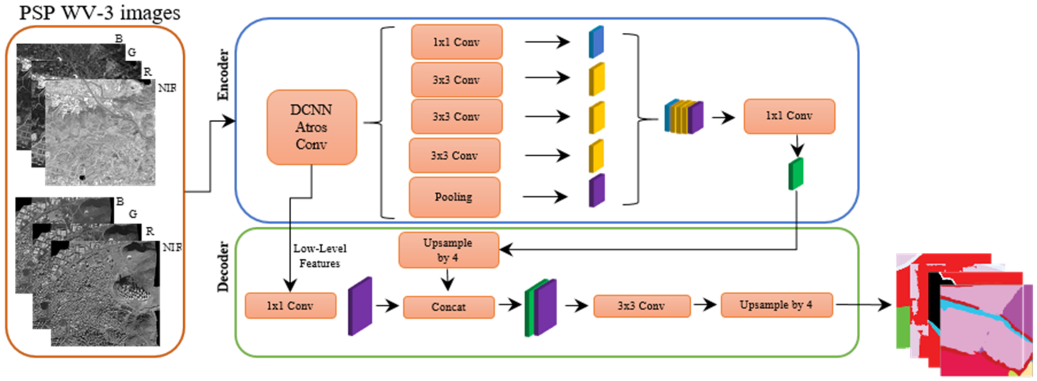
All the codes are implemented in the Pytorch (1.14.0) library, using the Python (3.8) programming language. The DNN models were trained and tested on a GeForce RTX 2080 Ti GPU. The DNN models constructed in this study are inherited from the FCN where the encoder part is followed by the decoder part, consecutively [32]. The encoder part is responsible for feature extraction from the input image, while the decoder part up-samples the feature maps in the latent space back to the original input size. In this study, after conducting a benchmark study that pointed out the best performing architecture couple, the DeepLab v3+ architecture was used to produce densely predicted segmentation maps and the ResNeXt50_32x4d [18,32,33,34,35,36] was used for the feature extraction from input images (i.e., mapping the input data into latent space). During the down-sampling that takes place in the encoder part, the low-level information extracted from the image in the embedded space is transferred to the decoder part with the use of Atrous convolutions. The training processes were limited to 150 epochs. The Adam optimization algorithm with a β value of 0.9 and a learning rate of 10−4 wereused to minimize the joint loss function, which consists of two distinct loss functions; Dice loss and Focal loss [37,38]. Equation (1) denotes the constructed loss function, where the first term represents the Dice loss and the second one is the Focal loss weighted with a coefficient of 0.5. Both functions adopted in this joint loss function are useful to cope with the aforementioned class imbalance problem (see Figure 4) in the dataset, as they assisted the model in focusing more on the samples that had not been sufficiently trained yet. In the Dice loss function, p i and g i represent the matched pixel values of prediction and ground truth, respectively. The a t term in the Focal loss function is a weighted-hyperparameter offset that scales the main term to address the class imbalance problem. The operator γ functions as a relaxation parameter that adjusts the importance given to correctly or wrongly classified samples.
L = 2 i N p i g i i N p i 2 + i N g i 2 + a t 1 p t γ log log p t   ×   0.5
Augmentation techniques are adopted by applying basic image processing techniques such as flip, rotation, shift, and scale with the intent of increasing the volume of the dataset. Besides, a sampling technique, where the under-represented samples are over-sampled, is used to help the model to focus more on under-represented classes. This technique is realized by feeding the weights calculated by sklearn’s compute_sample_weigh to the PyTorch’s DataLoader as an input [31]. Thus, the samples consisting of more class types are given more importance during the training phase. The workflow of this study is given in Figure 5.

3.2. Evaluation Metrics

Apart from qualitative analysis, widely-used evaluation metrics are adopted to assess the capability of the constructed classifiers. The quantitative analysis metrics used in this study are Intersection over Union (IoU), precision, recall, F1 score, and accuracy values calculated from the confusion matrix.
The F-1 score represents the harmonic mean of precision and recall scores, which measures the exactness and sensitivity abilities of the classifier. Unbalanced precision and recall scores result in a poor F-1 score, whereas having balanced precision and recall scores ensures a higher F-1 score. The formulation of precision, recall, and F-1 scores is described in Equations (2)–(4). TP represents true positive samples which belong to the same classes but in reference and classified data. FP represents false positive samples, which wrongly indicate that the related class is present, and FN represents false negative values, which wrongly indicate that the related class is not present.
Precision   = TP TP   +   FP
Recall   = TP TP   +   FN
F 1   score = 2 × Precision   ×   Recall Precision   +   Recall  
The IoU score assesses the classifier’s ability in terms of overlapping. The IoU score takes values between 0 and 1, the latter being the highest. The formulation of the IoU score is calculated as follows (Equation (5)),
IoU = A r e a   o f   O v e r l a p A r e a   o f   U n i o n
A confusion matrix, also known as an error matrix, is a table-wise representation of the number of classified/predicted and reference/actual/ground truth pixels, which are further used to calculate the overall, producer’s, and user’s accuracy values to quantitatively analyze the performance of a classification algorithm. The overall accuracy is an indication of the proportion of correctly mapped pixels considering all classes. The producer’s accuracy is used to evaluate how accurate real features on the ground are predicted in the classified map. The producer’s accuracy indicates the probability of a reference area being classified as accurate with the used classification model. This is mainly about the ability of the classification. The user’s accuracy indicates the probability of a classified pixel/segment actually representing that class on the ground. The user’s accuracy reflects the accuracy from the perspective of the map user, and it is more about the reliability [12,39].

3.3. Results and Discussion

A preliminary experimental analysis was conducted to find out the most appropriate segmentation model by comparing six well-known deep neural network architectures, which are:
  • DeepLabv3+ [40],
  • Pyramid Attention Network (PAN) [41,42],
  • U-Net++ [43],
  • Feature Pyramid Networks (FPNs) [44],
  • Linknet [45], and
  • Pyramid Scene Parsing Network (PSPNet) [41].
Quantitative results obtained from these architectures are shown in Table 2. We obtained the best performance with the DeepLabv3+ architecture; in which we achieved an IoU of 89.46%, an F-1 score of 94.35%, a precision of 94.25%, and a recall of 94.49%. The lowest metric values are obtained for PSPNet; in which the IoU is 71.20 %, the F-1 score is 82.44%, the precision is 82.44%, and the recall is 82.45%. PAN architecture is ranked as second and U-Net++ as third based on our experiment results.
We used the ResNeXt50_32x4d version of the ResNeXt50 encoder for the architecture search conducted in Table 2. Xie et al. [36] developed the ResNeXt models in which a building block aggregating a set of transformations is repeated for the construction of the network. They produced a homogenous, multi-branch architecture that required the setting of very few hyperparameters. ResNeXt includes a stack of residual blocks having the same topology and is subjected to two rules regarding spatial map down-sampling and computational complexity. The Resnext50_32x4d encoder utilizes a 7 × 7 convolutional layer with a stride of 2 for the creation of the first feature map. Then, each encoder step uses residual blocks, including a 1 × 1 convolutional layer, a 3 × 3 convolutional layer, a 1 × 1 convolutional layer, and the grouped convolutions of 32 [36,46].
We pursued our experiments with the first-ranked DeepLabv3+ architecture and evaluated the impact of different encoders on the segmentation task (Table 3) using the Aksu dataset. The encoder search experiment is aimed at finding the encoder-segmentation architecture pair that performs the best on the task we are addressing in this study. We implemented the below encoders with the DeepLabv3+ architecture:
  • Next generation ResNet (ResNeXt), resnext50_32x4d version with 22 M parameters and ImageNet weights,
  • Detail-Preserving Network (DPN), DPN68 version with 11 M parameters and ImageNet weights
  • EfficientNet, efficientnet-b0, efficientnet-b1, and efficientnet-b2 versions with 4M, 6M, and 7M parameters, respectively and having ImageNet weights.
  • MobileNet, mobilenet_v2 version with 2M parameters and ImageNet weights.
Table 3. Comparison of the Encoders using the DeepLabv3+ segmentation architecture (bold font indicates the bests performing setup).
ArchitectureParametersIoUF1 ScorePrecisionRecall
ResNeXt5022M89.4694.3494.2594.49
ResNet5023M87.3293.0892.9993.16
DPN6811M80.8388.6188.6188.61
MobileNet v22M79.0788.0988.1588.02
Efficientnet-b04M79.9488.4888.4288.55
Efficientnet-b16M82.6490.2490.1690.32
Efficientnet-b27M83.3690.5890.5290.64
In Figure 6, we illustrate the input image patches, the related ground truth data, and visual results of Resnext50_32x4d, Resnet50, DPN-68, Mobilenetv2, and Efficientnet encoders. For Efficientnet, we included results from Efficientnet-b2, which provided the highest accuracy. In general, the Resnext50_32x4d and Resnet50 encoders provided better predictions than other encoders.
The selected encoders shown in Table 3 vary in parameter size and adopted architecture strategy, making the comparison far-reaching. After determining the best-performing architecture pair as DeepLabv3+ and ResNext50_32x4d, where the former architecture constructs the encoder–decoder structure and the latter creates latent space representation of the input data within the context of feature extraction, we continued with applying the DNN model to three different datasets explained in the previous section and provided accuracy metrics in Table 4. We obtained the best performance for the Aksu dataset with an IoU of 89.46% and an F-1 score of 94.35%, which includes ten LULC classes shown in Figure 3a. Whereas, we obtained an IoU value of 81.64% for the Kestel dataset, which is quite lower than the Aksu dataset. This is due to the presence of more LULC classes (thirteen classes, as can be seen in Figure 3b) in this region. When we combine both datasets (Aksu and Kestel) and form an integrated dataset (herewith Aksu + Kestel), we have thirteen classes in total, with more patches from two different regions. This integration improved the IoU value up to 86.92%, emphasizing the importance of having more geographically diverse patches in a higher volume (Table 4). However, this value is lower than the IoU value of the Aksu dataset, supporting our interpretation of the decrease in the overall accuracy with the increase in the number and diversity of LULC classes. The behavior (the Aksu + Kestel dataset performance lagging behind the Aksu dataset) could be explained by the degree of the class imbalance the datasets are suffering from. Another explanation could be the effect of a geographical domain shift that dampens the performance.
When we evaluated the class-wise accuracy values of the classifier trained on the Aksu dataset (Table 5), we obtained 0.886 and higher accuracy values for all of the classes except for the road and rail class. This class is mostly mixed with heterogonous agricultural areas and then the forest class based on the analysis of the confusion matrix. Moreover, the mine, dump, and construction sites class is also mixed with the forest class to some extent for the Aksu dataset.
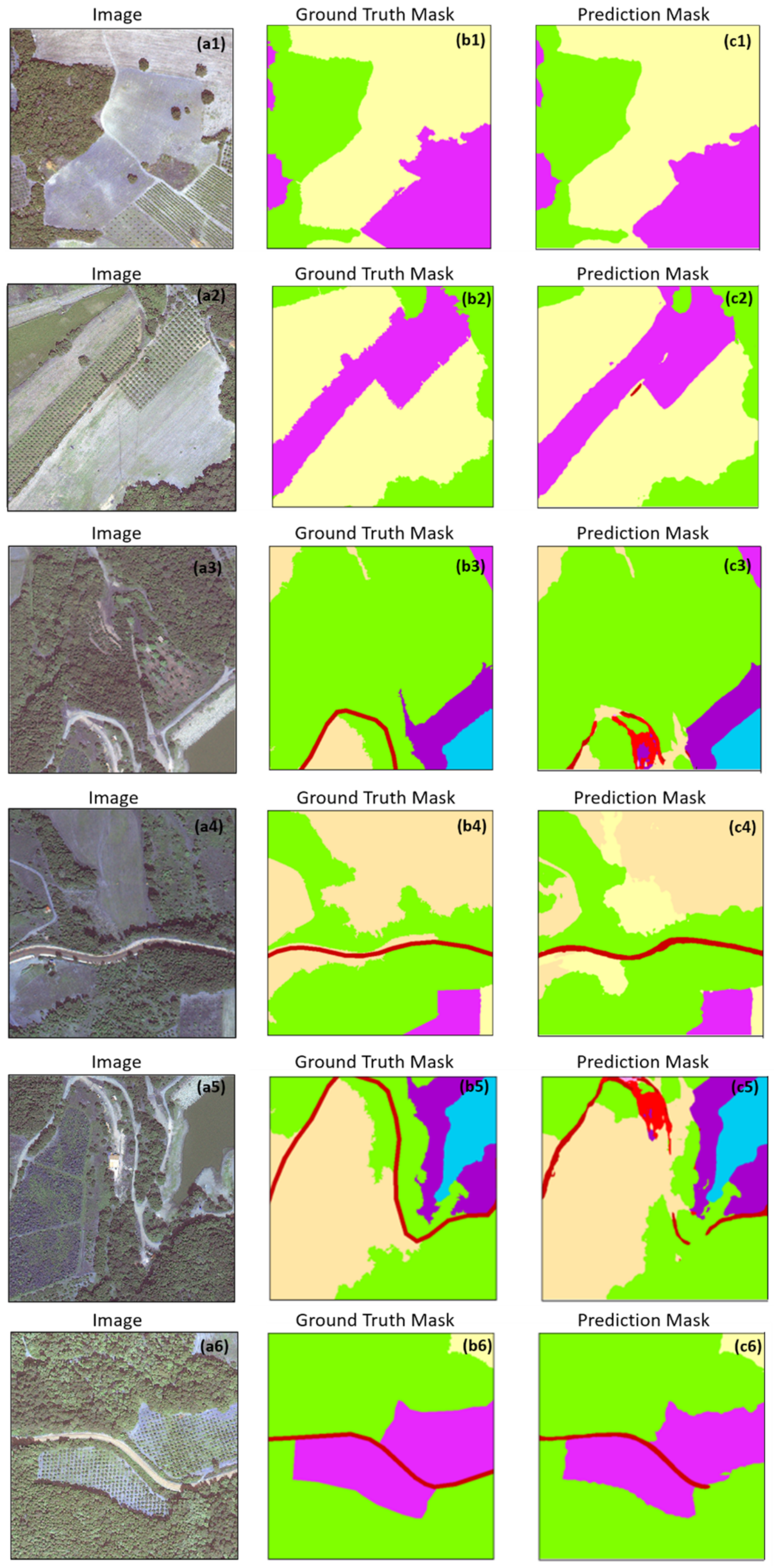
We further evaluated our results qualitatively and provided some visual analysis by generating figures (Figure 7, Figure 8 and Figure 9). As an example, in Figure 7, the first two image patches Figure 7a1,a2 covering forest, arable land, and permanent crops are successfully classified with our DNN setup. We included more samples from the road and rail class since we detected confusion in this class in the error matrix. Our analysis showed that there are some simplifications for roads in the ground truth data, specifically Figure 7a3,a5, which cannot be fully captured by the DL-based classifier. Yet, this might be acceptable when we analyze the input image characteristics. On the other hand, the road and rail class in the case of highways can be identified as shown in Figure 7a4–c4,a6–c6.
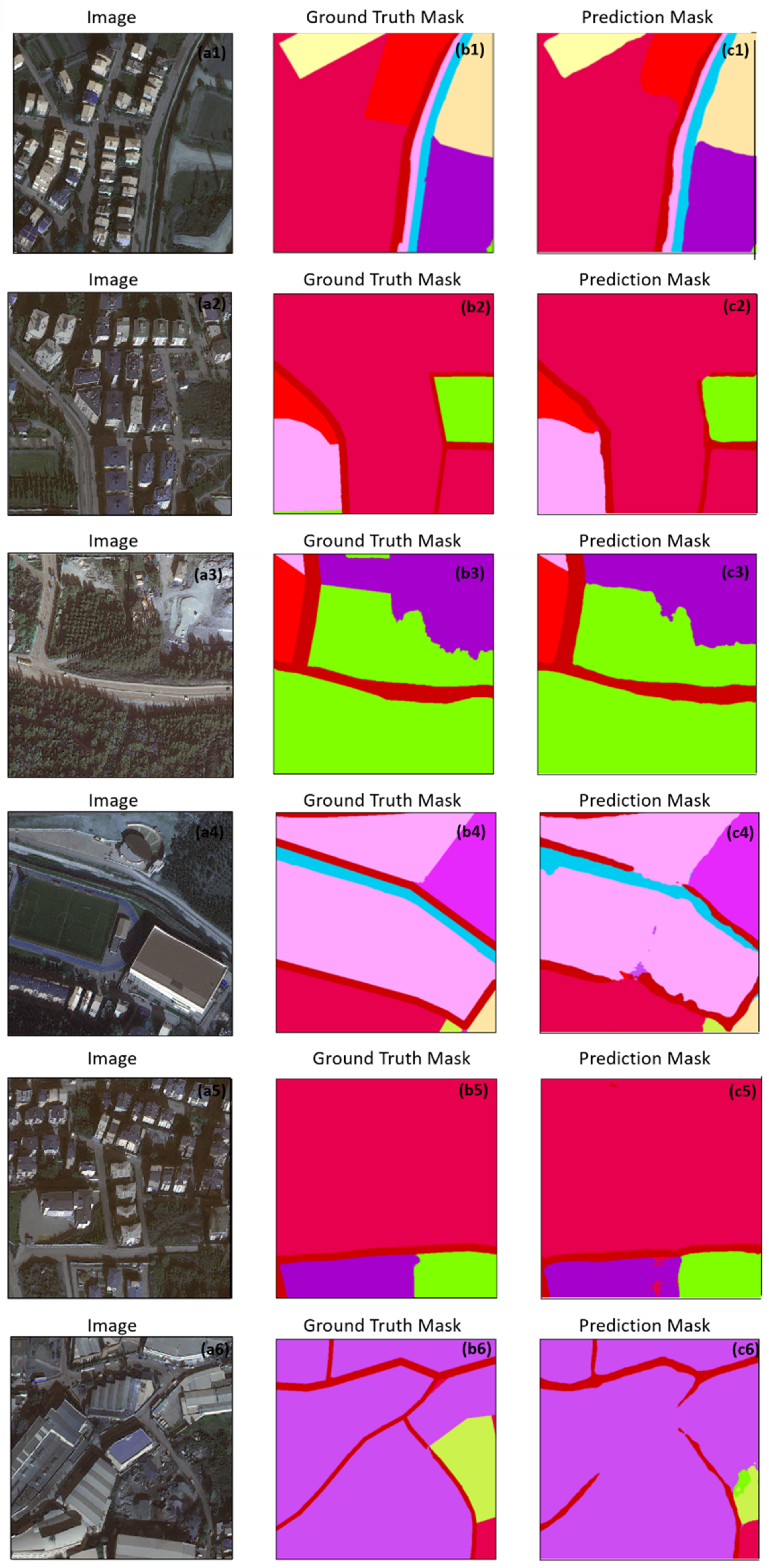
The analysis of the confusion matrix of the classifier trained on the Kestel dataset shows that the DNN model struggles to classify road and rail networks (0.683) and shrub and/or herbaceous vegetation associations (0.250) classes, as can be seen in Table 5. The road and rail class is mixed with several different classes but mostly with industrial or commercial units and continuous urban fabric classes, and with the forest class to some extent. The class-wise accuracy of the shrub and/or herbaceous vegetation is very low. This class is mostly mixed with industrial and commercial units. The overall class accuracy of inland water is 0.809 in the Kestel dataset, and this is lower than the overall inland class accuracy of the Aksu dataset, which is 0.983. The inland water class is confused with artificial, non-agricultural vegetated areas in the Kestel dataset. This region is dominated by urban-related classes and the overall accuracy of continuous urban fabric is quite good with a value of 0.986. The qualitative results of the classifier trained on the Kestel dataset are presented in Figure 8.
In most cases, the DNN model predicted the LULC classes accurately in the Kestel region, specifically over continuous urban fabric areas such as Figure 8c1,c2,c5. The DNN model has problems with the road and rail class, specifically for the roads occluded by building shadows (Figure 8a6,c6). In addition, similar to the Aksu dataset, highways as a part of the road and rail class could be successfully identified in the Kestel dataset, as seen in Figure 8a3–c3.
There is an improvement in class-wise accuracy values of the combined dataset at least better than one of the individual datasets and, in some cases, even better than both individual datasets (Table 5). As an example, if we analyze the discontinuous urban fabric class, the class-wise accuracies are 0.894 and 0.794 for the Aksu and Kestel datasets, respectively. The accuracy value obtained with the combined dataset in this class is 0.847, which is better than the Kestel dataset but worse than the Aksu dataset. In most of the classes, except for the artificial and non-agricultural associations, the Aksu + Kestel dataset performs better compared to individual datasets (the Aksu and Kestel datasets). The artificial and non-agricultural associations class is mostly mixed with the continuous urban fabric class in the combined dataset.
The class-wise accuracy of the forest class is the best in the combined dataset. The road and associated networks and the shrub and herbaceous vegetation associations classes are among the classes that significantly benefited from utilizing the classifier trained on the combination of Aksu and Kestel datasets. Although the total number of shrub and herbaceous vegetation association class patches did not increase in the combined dataset, the overall accuracy of this class improved dramatically, pointing out that having more patches from other classes, specifically those mixed with the shrub class, also contributes to the improvement of the classification results.
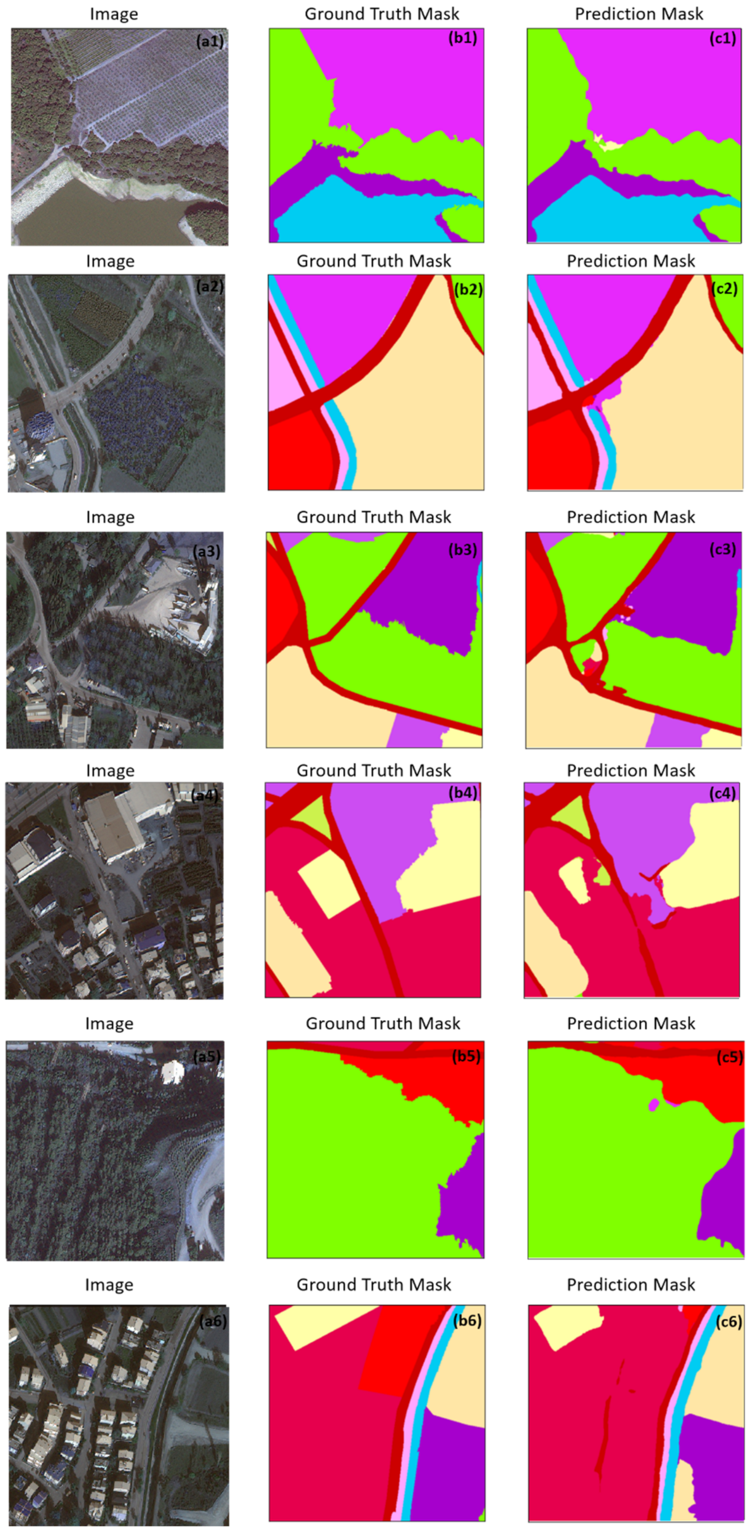
We assessed the visual results of the combined Aksu + Kestel dataset for different classes (Figure 9). Figure 9a1 covers a patch of permanent crops, forest, and an inland water region. The DNN model could successfully segment these different class combinations within the same patch, which can be easily seen with the match of the ground truth Figure 9b1 and prediction Figure 9c1. The road and rail class pixels could be successfully distinguished in this dataset, as can be seen in Figure 9a2,a3,b2,b3,c2,c3.
We cannot directly compare our outcomes with the results in the literature since our dataset is different in terms of satellite images that we use and the number and definition of LULC classes that we implemented. Unlike common practice, in which GT is digitized manually during the labeling task; in this research, the GT data in the dataset have been curated first by running GEOBIA classification and then manually revising the resulting classified segments, resulting in high-quality annotated LULC classes that describe the surface accurately. This strategy for curating the GT data is of novel value and takes our study into a different venue compared to the most DL-based LULC studies. Having weakly-labelled GT data gives rise to the deployment and development of weakly-supervised methods on our dataset.
However, when we concentrate on other research used VHR images specifically WV-3 and had common LULC with ours, we observe superiority of the DNN configured for this study given the fact that our dataset is annotated with higher number of LULC classesApart from the rich intra-diversity of the classes it contains, our dataset is also a test-bed to develop methods that are aimed at addressing the domain shift phenomenon, which is driven by a geographical shift in this case. As the GT annotations are labelled in a coarse and weak manner, in addition to the main full-supervision frame, we further propose our dataset as a benchmark for weak supervision methods. This performance, we argue, is strongly related to the diverse and versatile nature of the dataset we curated. Zhang et al. [47] employed the Atrous spatial pyramid pooling (ASPP)-UNet model for the identification of five different LULC classes and one other class. They trained and tested their proposed model using WorldView-2 (WV-2) and WV-3 images in Beijing city. They achieved an 84.0% overall accuracy for WV-3 test images for six classes. Considering that they used similar VHR images to our study, we further looked into class-wise accuracy in the common classes. They obtained F-1 values of 0.906 and 0.755 for the water and road classes, respectively, which are lower than our combined Aksu + Kestel dataset test results (Table 5). Bengana et al. [48] used Sentinel-2, WV-2, and Pleiades-1B satellite images and used a generalized CORINE Land Cover nomenclature as ground truth. They used six LULC classes, which were a combination of different LULC classes that we used in our research. For example, they combined different urban density classes, industrial, and mine-related classes under a common class called urban. They also combined all agricultural classes, such as arable land, permanent crops, and heterogenous areas, under a common class of agriculture. The mean IoU value that they obtained for six classes for WV-2 images was 55.59, whereas we obtained an average IoU value of 86.91 for twelve LULC classes. Kemker et al. [25] used VHR UAV images to identify eighteen different classes, which are mostly at the object level. The overall accuracy that they achieved was 59.8%, which is lower than the overall accuracy that we obtained in this research. This is an important finding to support, even with the availability of highly detailed UAV images, the segmentation task is becoming demanding with the increasing complexity and number of land classes.

4. Conclusions

In this paper, we first introduce a dataset for the task of land use land cover classification, andpresent comparisons of different deep learning-based segmentation architectures and encoders for land use and land cover mapping of VHR satellite images. We implemented an off-the-shelf model l (the DeepLabv3+ architecture withResNeXt50 encoder) to two different geographical locations having different topographical and landscape structures to analyze the generalization capabilities of the models. We focused on twelve distinct LULC classes, corresponding to the second level of the semantic hierarchy defined by CORINE nomenclature. Unlike common practice, the GT data was produced using GEOBIA approach and comprised LULC classes that weakly describe the surface in a less fine-detailed manner. Thus, we propose our dataset as a test-bed to further develop weakly-supervised methods, which is a pressing need in computer science research.
The novelty of our dataset lies not only in the annotation strategy adopted but also in the inclusive selection of the classes present in the dataset. Further, the dataset we introduce in this paper consists of twelve complex classes which are capable of adequately covering the complexity of the Earth’s surface, which further promotes the real-life applicability of the methods developed in our dataset. The curated dataset could also be used as a test-bed to assess the generalizability of the developed DNN models, given the multi-location asset of the images.
The DNN model used in this study achieves high accuracy for complex LULC classes, and this design could be implemented on different VHR satellite images or different geographical regions to generate accurate LULC maps. These maps can be used in various applications, from regional planning to future land change projections.
Data availability has a significant role in deep learning applications. Although there are several datasets freely accessible for different DL tasks, specifically in terms of input images, having reliable reference or ground truth data is still problematic. We generated a new benchmark dataset to be used for segmentation tasks, which can be used as a reference for implementing new segmentation models via supervised, semi- or weakly-supervised deep learning models. In addition, our model results can be used for transfer learning and the generalization of different methodologies.

Author Contributions

Conceptualization, E.S. and B.E.; methodology, E.S., B.E. and P.E.O.; software, B.E. and P.E.O.; validation, E.S., and B.E.; formal analysis, B.E. and P.E.O.; investigation, E.S., B.E., M.E.K. and P.E.O.; resources, E.S. and M.E.K.; data curation, B.E. and P.E.O.; writing—original draft preparation, E.S., B.E., M.E.K. and P.E.O.; writing—review and editing, E.S., B.E., M.E.K. and P.E.O.; visualization, B.E. and P.E.O.; supervision, E.S. and M.E.K.; project administration, E.S. and M.E.K.; funding acquisition, M.E.K. All authors have read and agreed to the published version of the manuscript.

Funding

This work was supported by the European Research Council (ERC) project: “Industrialisation and Urban Growth from the mid-nineteenth century Ottoman Empire to Contemporary Turkey in a Comparative Perspective, 1850–2000” under the European Union’s Horizon 2020 research and innovation program Grant Agreement No. 679097, acronym UrbanOccupationsOETR. M. Erdem Kabadayı is the principal investigator of UrbanOccupationsOETR.

Data Availability Statement

The dataset and model weights are publicly available at: https://github.com/RSandAI/LULCMapping-WV3images-CORINE-DLMethods (accessed on 1 February 2022).

Acknowledgments

We are thankful to the Maxar Technologies for Worldview-3 data provision. We also thank Cengiz Avci for his support on figure improvements.

Conflicts of Interest

The authors declare no conflict of interest.

References

  1. Sertel, E.; Topaloğlu, R.H.; Şallı, B.; Yay Algan, I.; Aksu, G.A. Comparison of landscape metrics for three different level land cover/land use maps. ISPRS Int. J. Geo-Inf. 2018, 7, 408. [Google Scholar] [CrossRef]
  2. Liu, Y.; Fan, B.; Wang, L.; Bai, J.; Xiang, S.; Pan, C. Semantic labeling in very high resolution images via a self-cascaded convolutional neural network. ISPRS J. Photogramm. Remote Sens. 2018, 145, 78–95. [Google Scholar] [CrossRef]
  3. Yuan, X.; Shi, J.; Gu, L. A review of deep learning methods for semantic segmentation of remote sensing imagery. Expert Syst. Appl. 2021, 169, 114417. [Google Scholar] [CrossRef]
  4. Xue, Z.; Li, J.; Cheng, L.; Du, P. Spectral–spatial classification of hyperspectral data via morphological component analysis-based image separation. IEEE Trans. Geosci. Remote Sens. 2015, 53, 70–84. [Google Scholar] [CrossRef]
  5. Ekim, B.; Sertel, E. Deep neural network ensembles for remote sensing land cover and land use classification. Int. J. Digit. Earth 2021, 14, 1868–1881. [Google Scholar] [CrossRef]
  6. Ettehadi Osgouei, P.; Sertel, E.; Kabadayı, M.E. Integrated usage of historical geospatial data and modern satellite images reveal long-term land use/cover changes in Bursa/Turkey, 1858–2020. Sci. Rep. 2022, 12, 9077. [Google Scholar] [CrossRef]
  7. Blaschke, T.; Hay, G.J.; Kelly, M.; Lang, S.; Hofmann, P.; Addink, E.; Queiroz Feitosa, R.; van der Meer, F.; van der Werff, H.; van Coillie, F.; et al. Geographic object-based image analysis—Towards a new paradigm. ISPRS J. Photogramm. Remote Sens. 2014, 87, 180–191. [Google Scholar] [CrossRef]
  8. Saha, S.; Bovolo, F.; Bruzzone, L. Unsupervised deep change vector analysis for multiple-change detection in VHR images. IEEE Trans. Geosci. Remote Sens. 2019, 57, 3677–3693. [Google Scholar] [CrossRef]
  9. Castillo-Navarro, J.; Le Saux, B.; Boulch, A.; Audebert, N.; Lefèvre, S. Semi-supervised semantic segmentation in Earth observation: The minifrance suite, dataset analysis and multi-task network study. Mach. Learn. 2021, 1–36. [Google Scholar] [CrossRef]
  10. Blaschke, T. Object based image analysis for remote sensing. ISPRS J. Photogramm. Remote Sens. 2010, 65, 2–16. [Google Scholar] [CrossRef] [Green Version]
  11. Qin, R.; Liu, T. A review of landcover classification with very-high resolution remotely sensed optical images—Analysis unit, model scalability and transferability. Remote Sens. 2022, 14, 646. [Google Scholar] [CrossRef]
  12. Topaloğlu, R.H.; Aksu, G.A.; Ghale, Y.A.G.; Sertel, E. High-resolution land use and land cover change analysis using GEOBIA and landscape metrics: A case of Istanbul, Turkey. Geocarto Int. 2021, 1–27. [Google Scholar] [CrossRef]
  13. Zhang, X.; Chen, G.; Wang, W.; Wang, Q.; Dai, F. Object-based land-cover supervised classification for very-high-resolution UAV images using stacked denoising autoencoders. IEEE J. Sel. Top. Appl. Earth Obs. Remote Sens. 2017, 10, 3373–3385. [Google Scholar] [CrossRef]
  14. de Pinho, C.M.D.; Fonseca, L.M.G.; Korting, T.S.; de Almeida, C.M.; Kux, H.J.H. Land-cover classification of an intra-urban environment using high-resolution images and object-based image analysis. Int. J. Remote Sens. 2012, 33, 5973–5995. [Google Scholar] [CrossRef]
  15. Chen, G.; Weng, Q.; Hay, G.J.; He, Y. Geographic object-based image analysis (GEOBIA): Emerging trends and future opportunities. GIScience Remote Sens. 2018, 55, 159–182. [Google Scholar] [CrossRef]
  16. Neupane, B.; Horanont, T.; Aryal, J. Deep learning-based semantic segmentation of urban features in satellite images: A review and meta-analysis. Remote Sens. 2021, 13, 808. [Google Scholar] [CrossRef]
  17. Merciol, F.; Faucqueur, L.; Damodaran, B.B.; Rémy, P.-Y.; Desclée, B.; Dazin, F.; Lefèvre, S.; Masse, A.; Sannier, C. GEOBIA at the terapixel scale: Toward efficient mapping of small woody features from heterogeneous VHR scenes. ISPRS Int. J. Geo-Inf. 2019, 8, 46. [Google Scholar] [CrossRef]
  18. Long, J.; Shelhamer, E.; Darrell, T. Fully Convolutional Networks for Semantic Segmentation. arXiv 2015, arXiv:1411.4038. [Google Scholar]
  19. Rottensteiner, F.; Sohn, G.; Jung, J.; Gerke, M.; Baillard, C.; Benitez, S.; Breitkopf, U. The ISPRS benchmark on urban object classification and 3D building reconstruction. ISPRS Ann. Photogramm. Remote Sens. Spat. Inf. Sci. 2012, I–3, 293–298. [Google Scholar] [CrossRef]
  20. ISPRS Potsdam 2D Semantic Labeling—Potsdam. 2019. Available online: https://www2.isprs.org/commissions/comm2/wg4/benchmark/2d-sem-label-potsdam/ (accessed on 1 February 2022).
  21. ISPRS Vaihingen 2D Semantic Label.—Vaihingen. 2019. Available online: https://www2.isprs.org/commissions/comm2/wg4/benchmark/2d-sem-label-vaihingen/ (accessed on 1 February 2022).
  22. Comp. Intelligence Group Hyperspectral Remote Sensing Scenes—Grupo de Inteligencia Computacional (GIC). 2019. Available online: http://www.ehu.eus/ccwintco/index.php?title=Hyperspectral_Remote_Sensing_Scenes#Pavia_Centre_and_University (accessed on 1 February 2022).
  23. Mnih, V. Mnih Massachusetts Building Dataset. Ph.D. Thesis, University of Toronto, Toronto, ON, Canada, 2013. [Google Scholar]
  24. Papadomanolaki, M.; Vakalopoulou, M.; Karantzalos, K. A Novel Object-based deep learning framework for semantic segmentation of very high-resolution remote sensing data: Comparison with convolutional and fully convolutional networks. Remote Sens. 2019, 11, 684. [Google Scholar] [CrossRef]
  25. Kemker, R.; Salvaggio, C.; Kanan, C. Algorithms for semantic segmentation of multispectral remote sensing imagery using deep learning. ISPRS J. Photogramm. Remote Sens. 2018, 145, 60–77. [Google Scholar] [CrossRef] [Green Version]
  26. Audebert, N.; Le Saux, B.; Lefèvre, S. Beyond RGB: Very high resolution urban remote sensing with multimodal deep networks. ISPRS J. Photogramm. Remote Sens. 2018, 140, 20–32. [Google Scholar] [CrossRef]
  27. Längkvist, M.; Kiselev, A.; Alirezaie, M.; Loutfi, A. Classification and segmentation of satellite orthoimagery using convolutional neural networks. Remote Sens. 2016, 8, 329. [Google Scholar] [CrossRef]
  28. Fu, G.; Liu, C.; Zhou, R.; Sun, T.; Zhang, Q. Classification for high resolution remote sensing imagery using a fully convolutional network. Remote Sens. 2017, 9, 498. [Google Scholar] [CrossRef]
  29. Zhang, Y. A new automatic approach for effectively fusing landsat 7 as well as IKONOS images. IEEE Int. Geosci. Remote Sens. Symp. 2002, 4, 2429–2431. [Google Scholar] [CrossRef]
  30. Wang, P.; Sertel, E. Channel–spatial attention-based pan-sharpening of very high-resolution satellite images. Knowl. Based Syst. 2021, 229, 107324. [Google Scholar] [CrossRef]
  31. Sklearn Package. Available online: https://scikit-learn.org/stable/about.html#citing-scikit-learn (accessed on 1 February 2022).
  32. Ekim, B.; Sertel, E.; Kabadayı, M.E. Automatic Road extraction from historical maps using deep learning techniques: A regional case study of Turkey in a German World War II Map. Int. J. Geo-Inf. 2021, 10, 492. [Google Scholar] [CrossRef]
  33. Ronneberger, O.; Fischer, P.; Brox, T. U-Net: Convolutional networks for biomedical image segmentation. In Proceedings of the Medical Image Computing and Computer-Assisted Intervention—MICCAI 2015, Munich, Germany, 5–9 October 2015; Navab, N., Hornegger, J., Wells, W.M., Frangi, A.F., Eds.; Springer International Publishing: Cham, Switzerland, 2015; pp. 234–241. [Google Scholar] [CrossRef]
  34. Avci, C.; Sertel, E.; Kabadayı, M.E. Deep Learning Based Road Extraction from Historical Maps. IEEE Geosci. Remote Sens. Lett. 2022, PP, 1. [Google Scholar] [CrossRef]
  35. Chen, L.-C.; Papandreou, G.; Schroff, F.; Adam, H. Rethinking atrous convolution for semantic image segmentation. arXiv 2017, arXiv:1706.05587. [Google Scholar]
  36. Xie, S.; Girshick, R.; Dollár, P.; Tu, Z.; He, K. Aggregated residual transformations for deep neural networks. In Proceedings of the 2017 IEEE Conference on Computer Vision and Pattern Recognition (CVPR), Honolulu, HI, USA, 21–26 July 2017; pp. 5987–5995. [Google Scholar] [CrossRef]
  37. Sudre, C.H.; Li, W.; Vercauteren, T.; Ourselin, S.; Cardoso, M.J. Generalised dice overlap as a deep learning loss function for highly unbalanced segmentations. arXiv 2017, arXiv:1707.03237. [Google Scholar] [CrossRef] [Green Version]
  38. Mulyanto, M.; Faisal, M.; Prakosa, S.W.; Leu, J.-S. Effectiveness of focal loss for minority classification in network intrusion detection systems. Symmetry 2021, 13, 4. [Google Scholar] [CrossRef]
  39. Congalton, R.G. A review of assessing the accuracy of classifications of remotely sensed data. Remote Sens. Environ. 1991, 37, 35–46. [Google Scholar] [CrossRef]
  40. Chen, L.-C.; Zhu, Y.; Papandreou, G.; Schroff, F.; Adam, H. Encoder-decoder with atrous separable convolution for semantic image segmentation. In Computer Vision—ECCV; Ferrari, V., Hebert, M., Sminchisescu, C., Weiss, Y., Eds.; Springer International Publishing: Cham, Switzerland, 2018; Volume 11211, pp. 833–851. ISBN 978-3-030-01233-5. [Google Scholar]
  41. Zhao, H.; Shi, J.; Qi, X.; Wang, X.; Jia, J. Pyramid scene parsing network. arXiv 2017, arXiv:1612.01105. [Google Scholar]
  42. Li, H.; Xiong, P.; An, J.; Wang, L. Pyramid attention network for semantic segmentation. arXiv 2018, arXiv:1805.10180. [Google Scholar]
  43. Zhou, Z.; Siddiquee, M.M.R.; Tajbakhsh, N.; Liang, J. UNet++: A nested U-Net architecture for medical image segmentation. arXiv 2018, arXiv:1807.10165. [Google Scholar]
  44. Lin, T.-Y.; Dollár, P.; Girshick, R.; He, K.; Hariharan, B.; Belongie, S. Feature pyramid networks for object detection. arXiv 2017, arXiv:1612.03144. [Google Scholar]
  45. Chaurasia, A.; Culurciello, E. LinkNet: Exploiting encoder representations for efficient semantic segmentation. In Proceedings of the 2017 IEEE Visual Communications and Image Processing (VCIP), St. Petersburg, FL, USA, 10–13 December 2017; pp. 1–4. [Google Scholar] [CrossRef]
  46. Ghosh, S.; Huo, M.; Shawkat, M.S.A.; McCalla, S. Using convolutional encoder networks to determine the optimal magnetic resonance image for the automatic segmentation of Multiple Sclerosis. Appl. Sci. 2021, 11, 8335. [Google Scholar] [CrossRef]
  47. Zhang, P.; Ke, Y.; Zhang, Z.; Wang, M.; Li, P.; Zhang, S. Urban land use and land cover classification using novel deep learning models based on high spatial resolution satellite imagery. Sensors 2018, 18, 3717. [Google Scholar] [CrossRef]
  48. Bengana, N.; Heikkila, J. Improving land cover segmentation across satellites using domain adaptation. IEEE J. Sel. Top. Appl. Earth Obs. Remote Sens. 2021, 14, 1399–1410. [Google Scholar] [CrossRef]
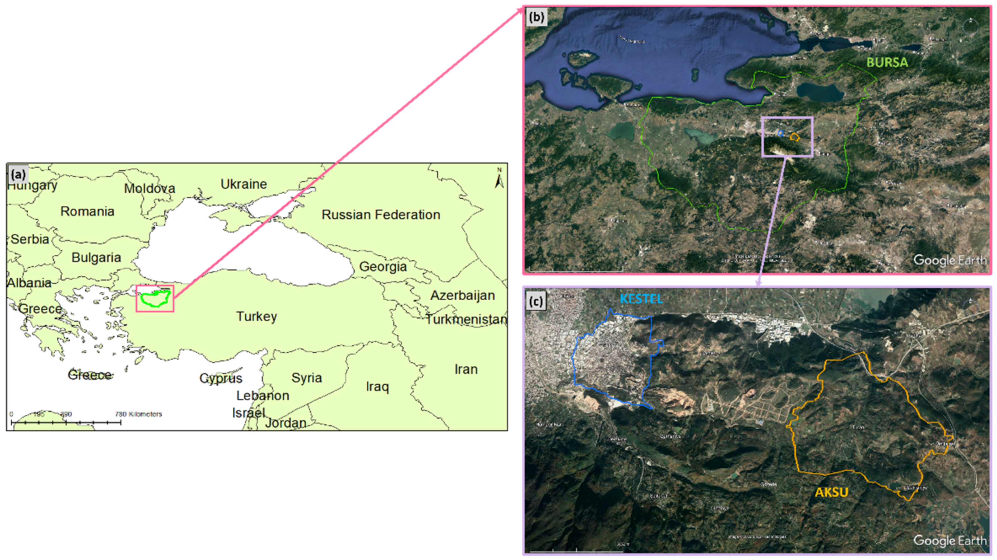
Figure 1. (a) General view of the study area and its surroundings. (b) The administrative boundary of Bursa province. (c) The administrative boundaries of Aksu and Kestel sites used in the research.
Remotesensing 14 04558 g001
Figure 2. Sample patches from the WV-3 images of the study areas, representing different LULC classes adapted from CORINE second-level nomenclature. (a) Heterogeneous agricultural areas, (b) Arable land, (c) Industrial units, (d) Forest, (e) Permanent crops, (f) Inland waters, (g) Continuous urban fabric, (h) Discontinuous urban fabric, (i) Road and rail networks and associated land, (j) Shrub and/or herbaceous vegetation associations, (k) Artificial, non-agricultural vegetated areas, (l) Mine, dump, and construction sites.
Remotesensing 14 04558 g002
Figure 3. LULC classes and their class-wise distributions (a) Class legend, (b) Aksu dataset, (c) Kestel dataset.
Remotesensing 14 04558 g003
Figure 4. Sample image patches and their corresponding ground truth masks. (a) sample patches from the Aksu region, (b) sample patches from the Kestel region.
Remotesensing 14 04558 g004
Figure 5. Flowchart of the used deep neural network architecture which follows an encoder–decoder structure with Atrous convolutions that bypasses the low-level features to the decoder.
Remotesensing 14 04558 g005
Figure 6. Comparison of visual results of predictions from different encoders. (a) Input images, (b) Ground truth data, (c) Resnext50_32x4d results, (d) Resnet50 results, (e) DPN-68 results, (f) Mobilenetv2 results, and (g) Efficientnet-B2 results.
Remotesensing 14 04558 g006
Figure 7. Qualitative results of the classifier trained on the Aksu dataset. (a1a6) show original image patches; (b1b6) illustrate the corresponding Ground Truth masks, and (c1c6) show the prediction results with the proposed model.
Remotesensing 14 04558 g007
Figure 8. Qualitative results of the classifier trained on the Kestel dataset. (a1a6) show original image patches; (b1b6) illustrate the corresponding Ground Truth masks, and (c1c6) show the prediction results with the proposed model.
Remotesensing 14 04558 g008
Figure 9. Qualitative results of the classifier trained on the Aksu + Kestel dataset. (a1a6) show original image patches; (b1b6) illustrate the corresponding Ground Truth masks, and (c1c6) show the prediction results with the proposed model.
Remotesensing 14 04558 g009
Table 1. Details of Worldview-3 image patches of the two study sites.
DatasetNumber of ClassesNumber of PatchesNumber of Patches in Train/
Validation/Test Sets
Aksu10599419/120/60
Kestel13265185/53/27
Aksu + Kestel13784549/157/78
Table 2. Comparison of segmentation results of different architectures (bold font indicates the best performing setup).
ArchitectureIoUF-1 ScorePrecisionRecall
DeepLabv3+89.4694.3594.2594.49
PAN82.7890.3790.3490.47
U-Net++81.5489.5489.6389.45
FPN76.4586.3986.3986.38
Linknet74.7584.9984.9585.04
PSPNet71.2082.4482.4482.45
Table 4. Comparison of segmentation results on different datasets.
DatasetIoUF1 ScorePrecisionRecall
Aksu89.4694.3594.2594.49
Kestel81.6489.6589.7689.54
Aksu + Kestel86.9292.8592.8492.86
Table 5. Class-wise accuracy values obtained from different dataset experiments.
AksuKestelAksu + Kestel
Forest0.9520.9180.968
Mine, dump, and construction sites0.8660.9600.903
Road and rail0.6120.6830.779
Discontinuous urban fabric0.8940.7940.847
Arable land0.9320.8440.867
Heterogeneous agricultural areas0.9430.9310.919
Permanent crops0.9080.9170.850
Inland waters0.9830.8090.965
Artificial, non-agricultural vegetated areas0.9890.7150.671
Industrial or commercial units-0.9670.954
Shrub and/or herbaceous vegetation-0.2500.775
Continuous urban fabric-0.9860.983
Publisher’s Note: MDPI stays neutral with regard to jurisdictional claims in published maps and institutional affiliations.