A Novel Method for AI-Assisted INS/GNSS Navigation System Based on CNN-GRU and CKF during GNSS Outage

Abstract

In the fields of positioning and navigation, the integrated inertial navigation system (INS)/global navigation satellite systems (GNSS) are frequently employed. Currently, high-precision INS typically utilizes fiber optic gyroscopes (FOGs) and quartz flexural accelerometers (QFAs) rather than MEMS sensors. But when GNSS signals are not available, the errors of high-precision INS also disperse rapidly, similar to MEMS-INS when GNSS signals would be unavailable for a long time, leading to a serious degradation of the navigation accuracy. This paper presents a new AI-assisted method for the integrated high-precision INS/GNSS navigation system. The position increments during GNSS outage are predicted by the convolutional neural network-gated recurrent unit (CNN-GRU). In the process, the CNN is utilized to quickly extract the multi-dimensional sequence features, and GRU is used to model the time series. In addition, a new real-time training strategy is proposed for practical application scenarios, where the duration of the GNSS outage time and the motion state information of the vehicle are taken into account in the training strategy. The real road test results verify that the proposed algorithm has the advantages of high prediction accuracy and high training efficiency.

1. Introduction

Global Navigation Satellite systems (GNSS) can provide accurate position and velocity information in outdoor environments, and its errors do not accumulate over time [1]. The disadvantages are that it can only provide less accuracy attitude information, the output frequency is low (1–20 Hz), and it is vulnerable to environmental interference. In contrast, the Inertial Navigation System (INS) is less dependent on the environment, and relies entirely on the angular velocity and acceleration information that is measured by the Inertial Measurement Unit (IMU), which can provide high-frequency navigation information [2,3]. But the position error will disperse over time due to the integral acquisition of positional information, resulting large errors in navigation results. Therefore, combining the respective advantages of GNSS and INS to obtain the navigation results with high accuracy, high interference immunity, and high frequency is a hot topic of research in the field of navigation at present [4,5].

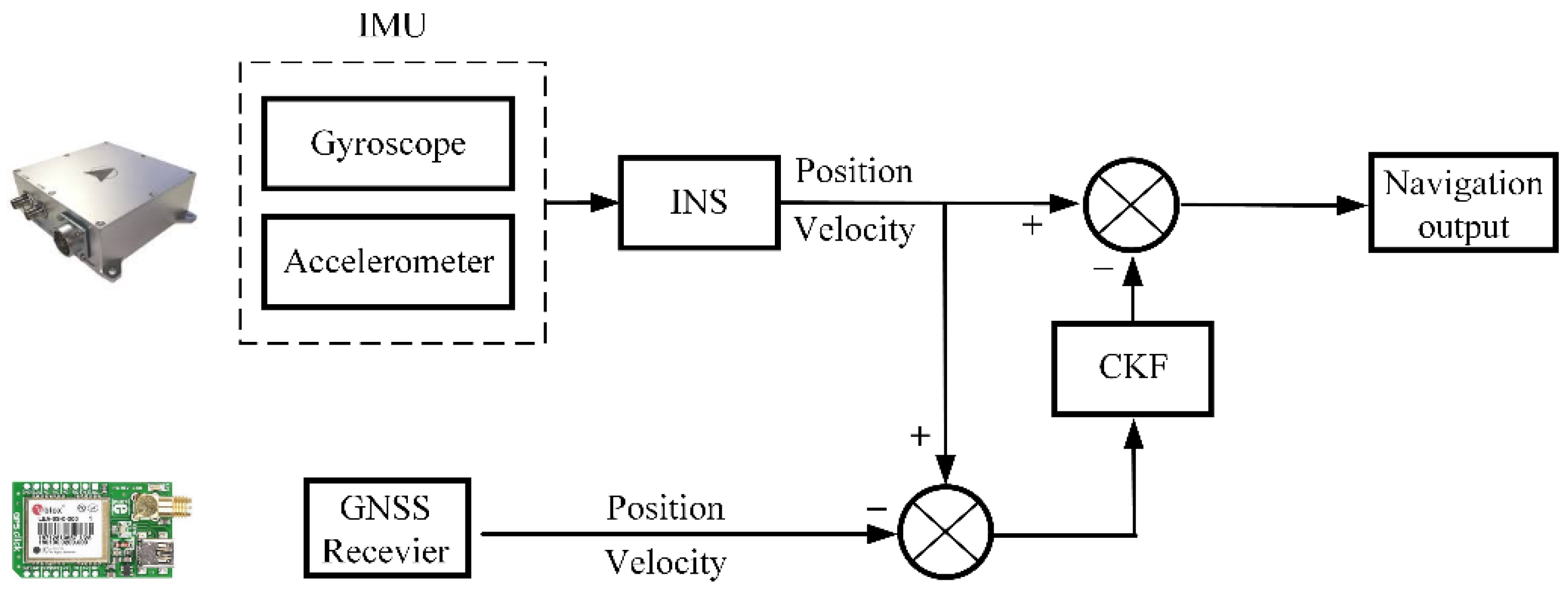
The Kalman filter (KF) and its upgrade variants are the most widely utilized algorithms for INS and GNSS information fusion [6,7]. The traditional Kalman filter algorithm can only be applied to linear systems, but most of the information in real navigation systems are nonlinear. Bucy et al. [8] proposed the extended Kalman filter (EKF), which linearizes the nonlinear function around the current estimate, and truncates the first-order linearization of the Taylor expansion of the nonlinear function. The remaining higher-order terms are ignored, and their performance depends on the degree of local nonlinearity. The unscented Kalman filter (UKF) was proposed to further improve the performance under nonlinear systems by making the nonlinear system equations applicable to linear assumptions through lossless transformations [9,10]. By approximating the posterior probability density of the state with a series of deterministic samples, the problem of the EKF accuracy dispersion under a highly nonlinear system is avoided. But the UKF has low accuracy in the high-dimensional case, the cubature Kalman filter (CKF) that is based on the spherical radial volume criterion is applied to data fusion, which can effectively approximate the Gaussian density function with higher accuracy, convenient parameter selection, and good convergence effect [11,12,13]. In order to improve the fusion accuracy in complex measurement environments, robust Kalman algorithms have also started to attract the attention of researchers [14,15]. To solve the problem of error model that is caused by measurement anomalies, Chen et al. [16] proposed a new cardinal maximum correlation entropy Kalman filter, which uses the robust maximum correlation entropy criterion (MCC) as the optimality criterion to solve the state estimation problem under outlier interference by maximizing the correlation entropy between states and measurements. Yun et al. [17] proposed a variational Bayesian-based state estimation algorithm to improve the CKF accuracy under dynamic model mismatch and outlier disturbance.

When the GNSS signals are unavailable, KF operates in predictive mode and corrects INS measurements according to the system error model. At this time, the accuracy of data fusion that relies only on the KF is not effective and navigation performance deteriorates rapidly. To improve the integrated navigation accuracy during GNSS outage, machine learning has started to be applied to integrated navigation systems. Ning et al. [18] proposed an optimal radial basis function (RBF)-based neural network that can improve the overall positioning accuracy during short-term GNSS signal outages. Hang et al. [19] proposed a new hybrid intelligence algorithm combining a discrete gray predictor (DGP) and a multilayer perceptron (MLP) neural network that provides pseudo-GPS positions during GNSS failures and uses GNSS position information from the last few moments to predict positions for future moments. Compared with traditional artificial neural networks, recurrent neural networks are more advantageous in combined navigation systems and can make full use of historical information [20,21,22]. Liu et al. [23] proposed a multi-channel long-short term memory (LSTM) network to predict the increments of vehicle position, which reduces the navigation error in case of GNSS outages by an order of magnitude. In practical applications, a large amount of historical data before the GNSS outage needs to be trained when the GNSS outage occurs, so the training efficiency of neural networks also has high requirements. Tang et al. [24] proposed a hybrid algorithm that was based on the gated recurrent unit (GRU) and adaptive Kalman filter (AKF), and the experimental results showed that GRU outperformed LSTM in terms of prediction accuracy and training efficiency. Zhi et al. [25] proposed a convolutional neural network-long short-term memory (CNN-LSTM) model, which uses convolutional neural network (CNN) to quickly extract the features of the input and LSTM network to output the pseudo-GPS signal, further improving the training efficiency. However, most of the current articles use the offline simulation, assuming that the GNSS failure time is known and do not consider the time that is required to train the model online. Al Bitar et al. [26] proposed a novel real-time training strategy for regular training on the past one minute data, with the disadvantage that only short historical data are used and the accuracy is poor when the time of GNSS outage is long.

To overcome the shortcomings of the traditional methods, our paper proposes a new AI-assisted method for the integrated high-precision INS/GNSS navigation system. The method consists of two parts: first, CKF is used to provide more accurate neural network training samples. Then, by building a CNN-GRU network to predict the position increments during GNSS outage, the CNN is utilized to quickly extract the multi-dimensional sequence features, and GRU is used to model the time series. In addition, a new real-time training strategy is proposed for practical application scenarios, where the duration of the GNSS outage time and the motion state information of the vehicle are taken into account in the training strategy. The experiments verify that the proposed algorithm has the advantages of high prediction accuracy and high training efficiency.

The rest of the paper is organized as follows: Section 2 introduces the INS error propagation model and the integrated navigation model that is based on CKF, Section 3 introduces the proposed CNN-GRU network, Section 4 performs the road test and result analysis, and the conclusion is presented in Section 5.

2. Mathematical Integrated System Model

The INS and GNSS are loosely coupled as shown in Figure 1. The INS and GNSS can complete position and velocity independently. Then, the position and velocity errors of INS are estimated using CKF, and these errors are used to correct the navigation output of INS and achieve the correction of gyro and accelerometer drift, thus reducing the impact of INS errors. In this section, we derive the error propagation model of INS, and then introduce the integrated navigation model that is based on CKF.

2.1. The Error Propagation Model

By integrating the angular velocity that is measured by gyro, the attitude direction of the inertial component can be obtained. By using the directional cosine matrix of the attitude direction, the specific force components of the accelerometer observations along each axis of the carrier system can be converted to the navigation coordinate system, the velocity and position can be calculated.

In the process of attitude calculation, the navigation coordinate system that is obtained is regarded as the real navigation coordinate system. In practice, due to the interference of various factors, the calculated navigation coordinate system will have deviations compared to the real navigation coordinate system, and the attitude error equation can be expressed as:

$$\dot{\varphi }=\varphi \times {\omega }_{in}^n+\delta {\omega }_{in}^n-\delta {\omega }_{ib}^n,$$

(1)

where $\delta {\omega }_{in}^n=\delta {\omega }_{ie}^n+\delta {\omega }_{en}^n$ is the angular velocity error in the navigation coordinate system, $\delta {\omega }_{ie}^n$ is the angular velocity error of the Earth’s rotation, $\delta {\omega }_{en}^n$ is the rotation error of the navigation system, $\delta {\omega }_{ib}^n=C_b^n\delta {\omega }_{ib}^b=C_b^n\left[\left(\delta K_G+\delta G\right){\omega }_{ib}^b+{\epsilon }^b\right]$ is the gyro measurement error, ${\epsilon }^b$ is the gyro drift error, and $\delta K_G$ and $\delta G$ are the gyro scale factor error and non-orthogonal installation error, which can be expressed as:

$$\begin{array}{l}\delta K_G=\mathrm{diag}\left(\left[\begin{array}{lll}\delta K_{Gx}\hfill & \delta K_{Gy}\hfill & \delta K_{Gz}\hfill \end{array}\right]\right)\\ \delta G=\left[\begin{array}{ccc}0& \delta G_z& -\delta G_y\\ -\delta G_z& 0& \delta G_x\\ \delta G_y& -\delta G_x& 0\end{array}\right]\end{array}$$

(2)

Both calibration residuals and installation errors can be considered as constants, while random drift can be expressed as a cumulative model of random constants and a first-order Markov model. In the presence of attitude error and specific force measurement error, the velocity differential error can be expressed as:

$$\delta {\dot{v}}^n=f_{sf}^n\times \varphi +\left(2\delta {\omega }_{ie}^n+\delta {\omega }_{en}^n\right)\times v^n-\left(2{\omega }_{ie}^n+{\omega }_{en}^n\right)\times \delta v^n+\delta f_{sf}^n+\delta g^n$$

(3)

where $\delta f_{sf}^n$ is the accelerometer measurement error, which can be expressed as the cumulative model of accelerometer zero deviation and white noise.

$$\delta g^n=\left[\begin{array}{c}0\\ -{\beta }_3\left(\sin 2L·\delta h+2h\cos 2L·\delta L\right)\\ -\left[g_e\sin 2L\left(\beta -4{\beta }_1\cos 2L\right)\delta L-{\beta }_2\delta h\right]\end{array}\right]$$

(4)

where $\beta$ is the gravity flattening, ${\beta }_1=2.32718\times {10}^{-5}{s}^{-2}$, ${\beta }_2=3.08\times {10}^{-6}{s}^{-2}$, ${\beta }_3=8.08\times {10}^{-9}{s}^{-2}$.

The position error is [27]:

$$\{\begin{array}{l}\delta \dot{L}=\frac{1}{R_M+h}\delta v_N-\frac{v_N}{{\left(R_M+h\right)}^2}\delta h\\ \delta \dot{\lambda }=\frac{\sec L}{R_N+h}\delta v_E+\frac{v_E\sec L\tan L}{R_N+h}\delta L-\frac{v_E\sec L}{{\left(R_N+h\right)}^2}\delta h\\ \delta \dot{h}=\delta v_U\end{array},$$

(5)

2.2. The Integrated Navigation Model Based on CKF

In the integrated navigation system, the CKF estimation is adopted to estimate the system state vector which is a 15 array vector:

$$X=[{\phi }_e {\phi }_n {\phi }_u \delta V_e \delta V_n \delta V_{\mathrm{u}} \delta L \delta \lambda \delta h {\nabla }_x {{\nabla }_y {\nabla }_z {\epsilon }_x {\epsilon }_y {\epsilon }_z]}^T$$

(6)

where ${\phi }_e$, ${\phi }_n$, and ${\phi }_u$ denote the attitude error angles of the INS in the east, north, and zenith directions. $\delta V_e$, $\delta V_n$, and $\delta V_{\mathrm{u}}$ denote the velocity error of INS in the three directions. $\delta L$, $\delta \lambda$, and $\delta h$ denote the latitude error, longitude error, and altitude error. ${\nabla }_x$, ${\nabla }_y$, and ${\nabla }_z$ are the accelerometer bias vectors, and ${\epsilon }_x$, ${\epsilon }_y$, and ${\epsilon }_z$ are the gyro bias vectors.

The equation of state and measurement equation of the system can be expressed as:

$$\{\begin{array}{l}\dot{X}=FX+GW\hfill \\ Z=HX+V\hfill \end{array}$$

(7)

where F is the system state transfer matrix, which consists of the INS system error. G is the system noise matrix. Z is the measurement vector, which is set to the position error vector and velocity error vector of INS and GNSS. H is the observation matrix. W is the process noise vector. V denotes the measured noise vector.

The CKF is based on the 3rd order volume rule and is suitable for high-dimensional filtering problems. The computation consists of two steps: the time update and measurement update phase, as shown in Algorithm 1.

Algorithm 1: Cubature Kalman Filter.

Require:${\widehat{x}}_{k-1\mid k-1},P_{k-1\mid k-1},Q_{k-1},R_k$ for$\mathrm{i}=1,\dots ,\mathrm{N}$do $\hspace{1em}{x}_{k-1}^i=S_{k-1\mid k-1}{\xi }_i+{\widehat{x}}_{k-1\mid k-1}$ $\hspace{1em}{w}_{k-1}^i=1/N$ end for Prediction phase: ${\widehat{x}}_{k\mid k-1}={\displaystyle \sum _{i=1}^N{w}_{k-1}^i}\mathrm{f}\left(x_{k-1}^i\right)$ $P_{k\mid k-1}={\displaystyle \sum _{i=1}^N{w}_{k-1}^i}\left(\mathrm{f}\left(x_{k-1}^i\right)-{\widehat{x}}_{k\mid k-1}\right){\left(\mathrm{f}\left(x_{k-1}^i\right)-{\widehat{x}}_{k\mid k-1}\right)}^T+Q_{k-1}$ for$i=1,\dots ,\mathrm{N}$do $\hspace{1em}{x}_{k\mid k-1}^i=S_{k\mid k-1}{\xi }_i+{\widehat{x}}_{k\mid k-1}$ $\hspace{1em}{w}_{k\mid k-1}^i=1/N$ end for Update phase: ${\hspace{1em}\hspace{1em}\widehat{z}}_{k\mid k-1}={\displaystyle \sum _{i=1}^N{w}_{k\mid k-1}^{\mathrm{i}}} \mathrm{h}\left(x_{k\mid k-1}^i\right)$ $\hspace{1em}\hspace{1em}{P}_{k\mid k-1}^{zz}={\displaystyle \sum _{i=1}^N{w}_{k\mid k-1}^i}\left( \mathrm{h}\left(x_{k\mid k-1}^i\right)-{\widehat{z}}_{k\mid k-1}\right){\left(\mathrm{h}\left(x_{k\mid k-1}^i\right)-{\widehat{z}}_{k\mid k-1}\right)}^T+R_k$ $\hspace{1em}\hspace{1em}{P}_{k\mid k-1}^{x\mathrm{z}}={\displaystyle \sum _{i=1}^N{w}_{k\mid k-1}^i}\left(x_{k\mid k-1}^i-{\widehat{x}}_{k\mid k-1}\right){\left(\mathrm{h}\left(x_{k\mid k-1}^i\right)-{\widehat{z}}_{k\mid k-1}\right)}^T$

3. CNN-GRU

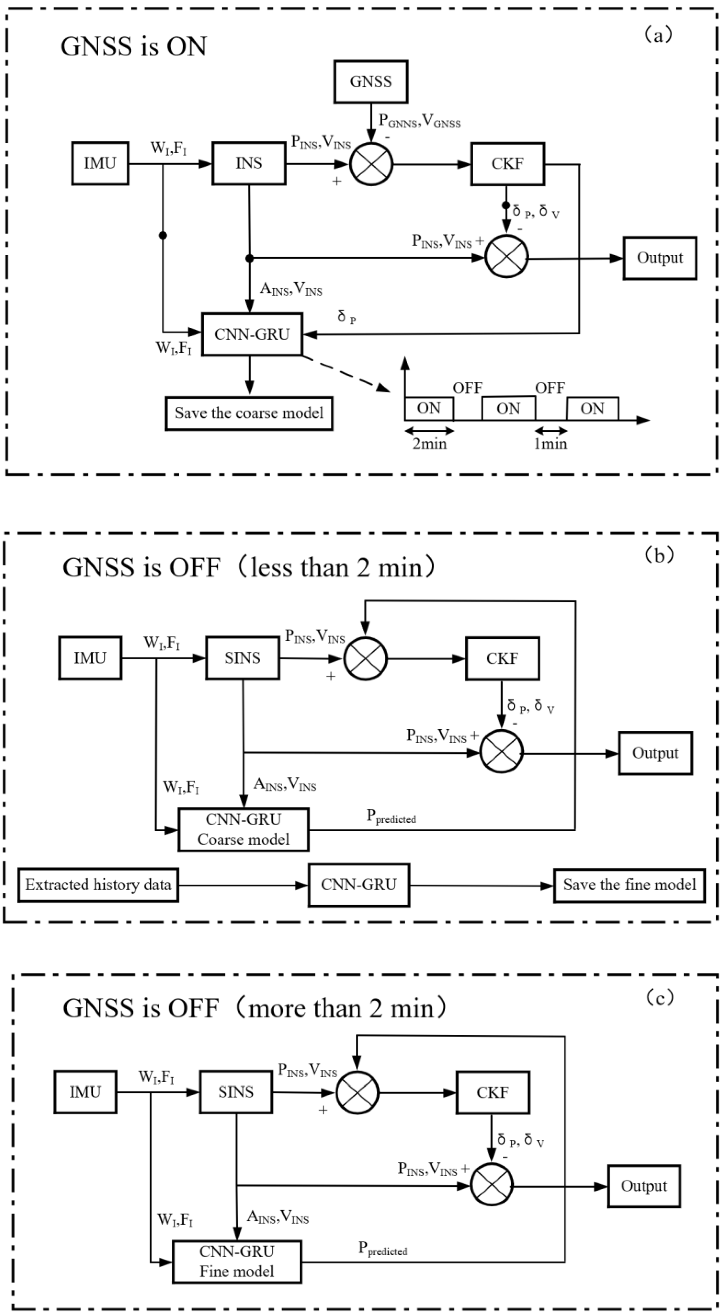
The overall architecture of our method is shown in Figure 2. In this paper, we use a loosely coupled integrated navigation scheme that is based on the combination of CKF and CNN-GRU. The CKF module provides highly accurate position, velocity, attitude, and IMU error information. The inputs and outputs of the network are shown in Figure 2, where $W_I$ and $F_I$ are the angular velocity and specific force that are provided by the IMU, $A_{INS}$ and $V_{INS}$ are the attitude and velocity information that is calculated by the INS. The outputs of the network are the position increments $\delta P$ output by the CKF module, which are integrated as the pseudo-GNSS position information. When the GNSS signals are available, the CNN-GRU module operates in learning mode. When the GNSS signals become unavailable, the CNN-GRU module operates in prediction mode, and the pseudo-GNSS position increments are predicted to ensure navigation accuracy. Specifically, three operating modes are included: learning mode when the GNSS signals are available, prediction mode and learning mode during GNSS short-term outage, and prediction mode during GNSS long-term outage. When the GNSS signals are available, the length of each learning sample is 2 min and the learning interval is controlled in 1 min. The reason for choosing – min is that most GNSS interruption scenarios last less than 2 min, and the purpose of the learning interval is to reset the CKF filter. When the GNSS signals are unavailable, the model that was trained in the previous phase is used for prediction, while the previous historical data are used for training the new fine model, and the model is switched to the new fine model to improve the prediction accuracy when the GNSS signals that are interrupted exceed 2 min. In order to ensure that the training of historical data can be completed within 2 min, we consider the differences of the model under different motion states of the vehicle and reduce the length of the training data. The decision is done using the vehicle motion state according to the output data of INS, which are zero speed, zero angular speed, zero lateral speed, and zero vertical speed, and stop saving data when a period of continuous motion state exceeds five minutes, thus improving the training efficiency.

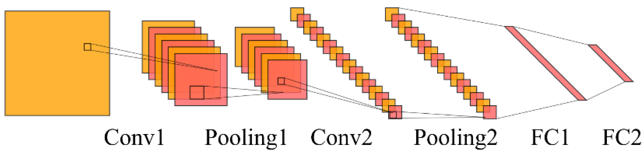
The CNN-GRU networks consist of a one-dimensional version of CNN, GRU, and a fully connected layer. Since the inputs involve multiple sensors and the coupling of multidimensional motion information, the intake features need to be extracted more accurately, so the CNN is used to quickly extract features from the sensor sequences. Since the vehicle motion and IMU sensor errors are time-dependent, the GRU is adopted to extract deeper hidden information from the sensor history data. Finally, a fully connected layer is used to obtain the final navigation information.

The structure of CNN is shown in Figure 3. CNN is one of the common network models in the field of deep learning, which is a multi-layer feedforward neural network with high generalization ability and robustness by local connectivity, weight sharing, and pooling operation [28]. The pooling layer is used to compress the high-dimensional features of the input after processing in the convolutional layer to reduce the parameter matrix dimension, which reduces the computational workload by reducing the parameters of the network. The fully connected layer can combine all of the local features into global features.

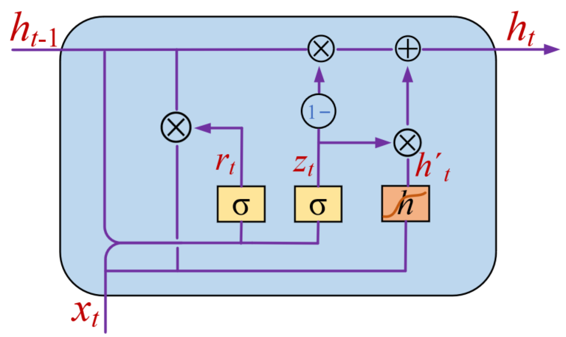
The GRU neural network is an improvement on the LSTM neural network. The LSTM neural network provides a new solution to the short-term memory problem and solves the problem of gradient disappearance and gradient explosion when the RNN exists to handle longer sequences. The GRU is simplified for the same estimation accuracy and higher training efficiency compared to the LSTM. The GRU model consists of two gates: the update gate and the reset gate. The update gate determines how much information from the previous state is brought into the current state. The larger the update gate is, the more the previous state is brought into the current state. The reset gate determines how the new input information is combined with the previous memory. The smaller the reset gate is, the more information about the previous state is ignored. The schematic diagram of GRU is shown in Figure 4.

GRU undertakes the most important task of sequence analysis, and the time-dependent nature of GRU makes training more difficult. Therefore, the core parameters are the size and structure of the GRU network. The hyperparameters that have the greatest impact on the performance include the number of GRU layers, the number of neurons, and the step size. Too many neurons lead to an overfitting phenomenon and degradation of the generalization performance, while insufficient number of neurons cannot fully extract the relationship between the input and output sequences, and too many GRU layers also lead to instability of the model. Considering the prediction accuracy and computation time, the number of GRU layers, the number of neurons, and the step size are set to 2, 48, and 2, respectively. The training time of the network increases with the above three hyperparameters. Two layers of GRU are sufficient to extract the hidden information, and too many layers can lead to overfitting.

4. Experiment Results

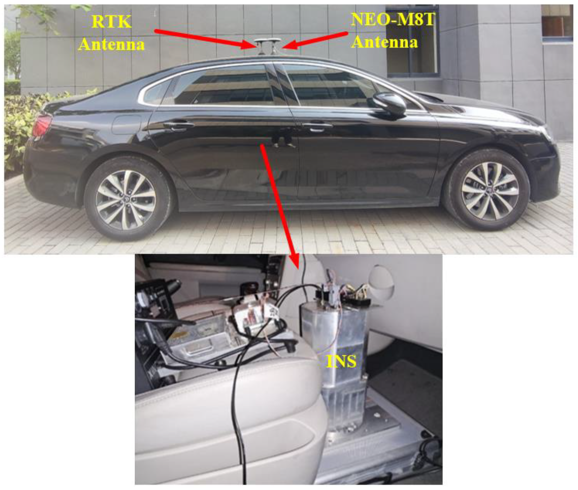
The road experiments were carried out on a vehicle platform using an INS/GNSS system, as shown in Figure 5. The INS system uses high-precision fiber optic gyroscope and quartz flexible accelerometer that was developed by our group. The GNSS receiver is Ublox NEO-M8T. The sampling frequency of the INS is set to 400 Hz, and the sampling frequency of the GNSS is 10 Hz. RTK GNSS provides the ground truth values. The specific parameters are shown in

Table 1. The parameters of the sensors.

Fiber optic gyroscope	Bias Scale factor Angular Random walk	0.02°/h 10 ppm 0.002°/$\sqrt{\mathrm{h}}$
Quartz Flexible Accelerometer	Bias Scale factor	10 ug 20 ppm
GNSS(Ublox NEO-M8T)	Position accuracy Velocity accuracy	2.5 m 0.05 m/s
RTK GNSS (NovAtel ProPak6)	Position accuracy	3 cm

. Two typical road experiments were carried out. After the initial alignment, the INS/GNSS was started in a loosely coupled integrated navigation mode. The experimental locations were in Zhejiang Province, China:

(1)

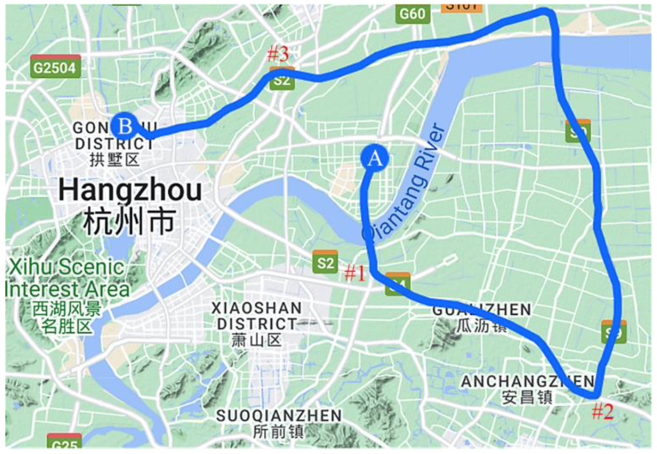
Experiment 1: Urban roads as shown in Figure 6: the duration of the experiment is 1 h, and the road conditions include straight lines, turns, and lane changes. There were three segments of simulated GNSS signals interruptions that were introduced, and the signal interruption durations were 60 s, 180 s, and 300 s, respectively.

(2)

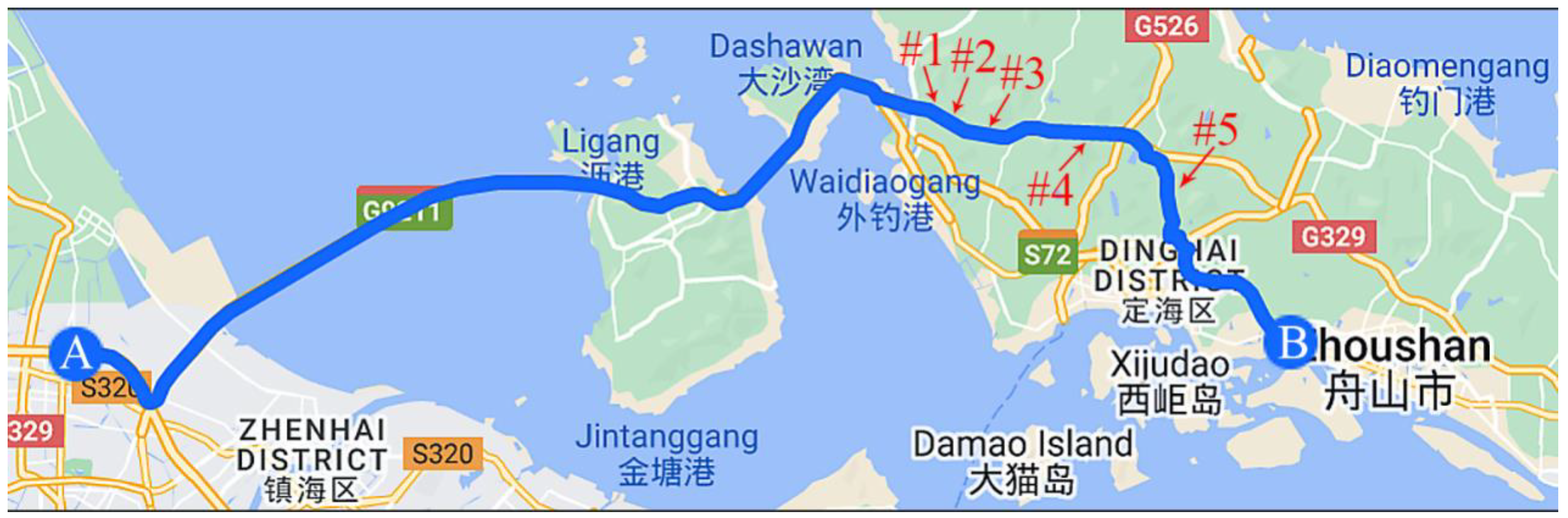
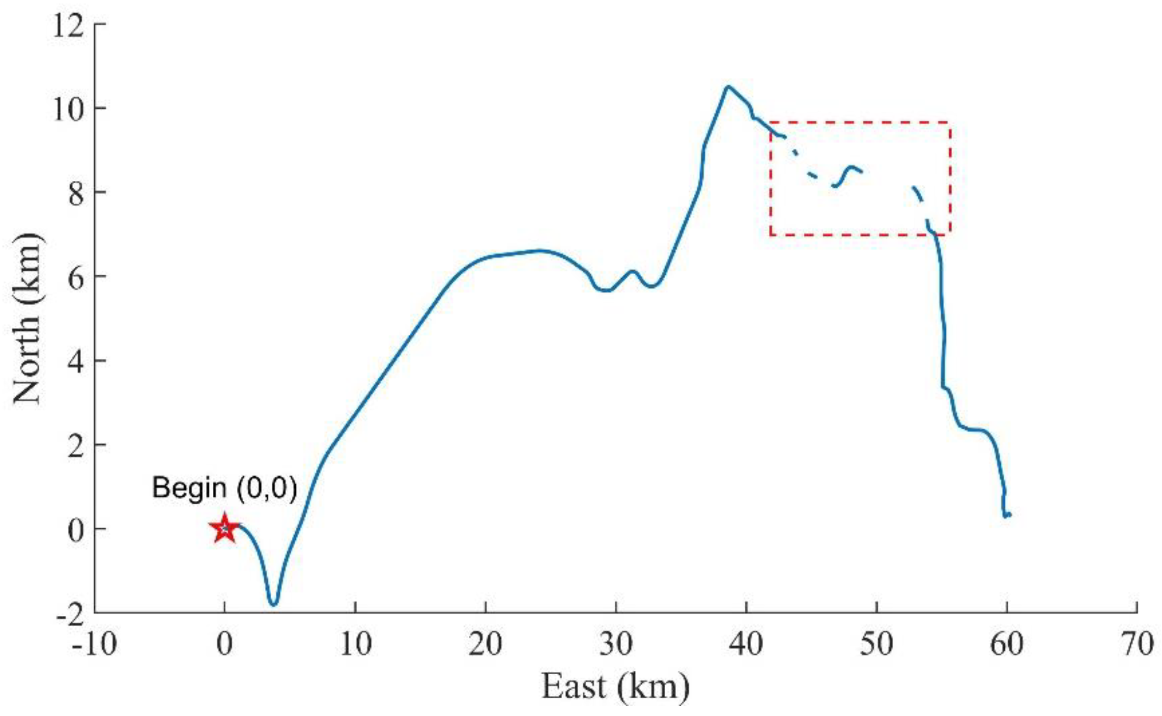
Experiment 2: Expressway including tunnels as shown in Figure 7: the duration of the experiment is 1 h, the road conditions are mainly long straight lines, and the driving trajectory contains multiple tunnels of different lengths to verify the performance of the proposed method in the case of real GNSS signals outage scenarios.

In order to verify the performance of the CNN-GRU-CKF that is proposed in our paper, we selected two typical road experiments, Experiment 1 focuses on urban roads, simulating GNSS interruptions by artificially turning off GNSS, while RTK is still working normally and can provide the ground truth of the position for verifying the algorithm accuracy. The GNSS signals interruption duration is 1 min, 3 min, and 5 min, respectively. In order to better reflect the effectivity of the algorithm, the trajectory containing the turn is deliberately chosen. When the GNSS signals are unavailable, the position information that is obtained by CNN-GRU prediction is used instead of the true GNSS information, and the measurement update process of CKF is carried out. Meanwhile, the performance of pure INS, MLP, and GRU is compared.

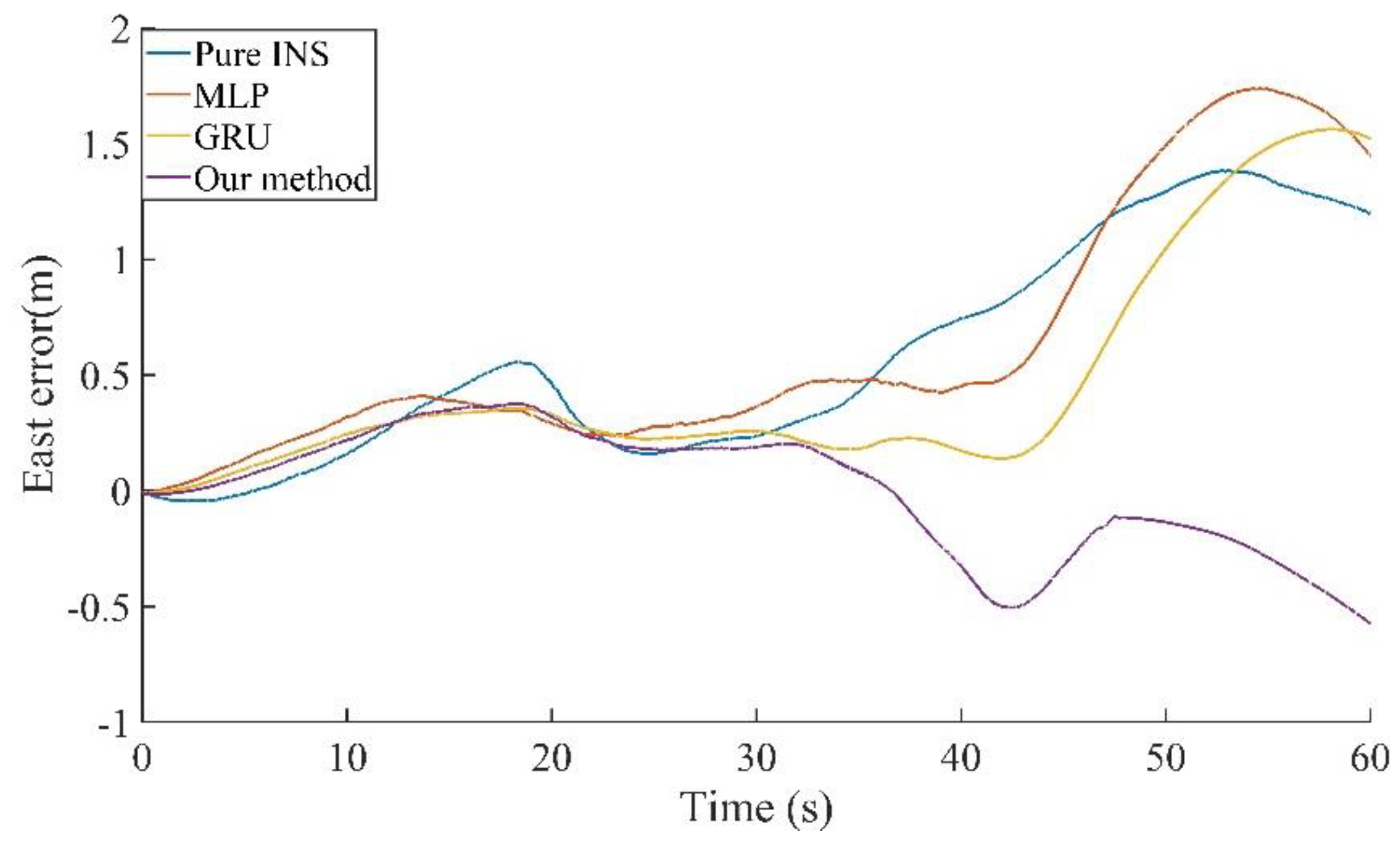
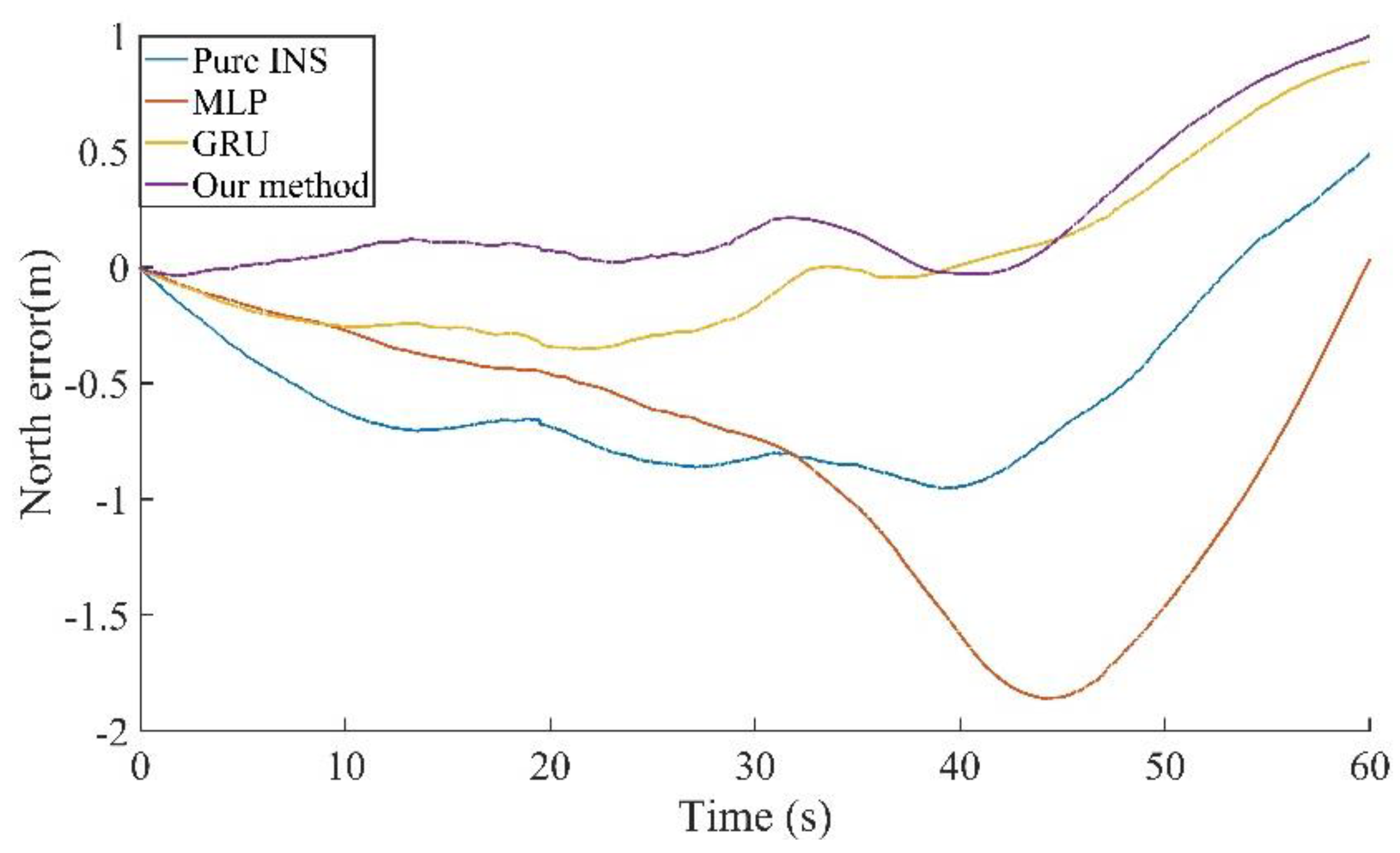
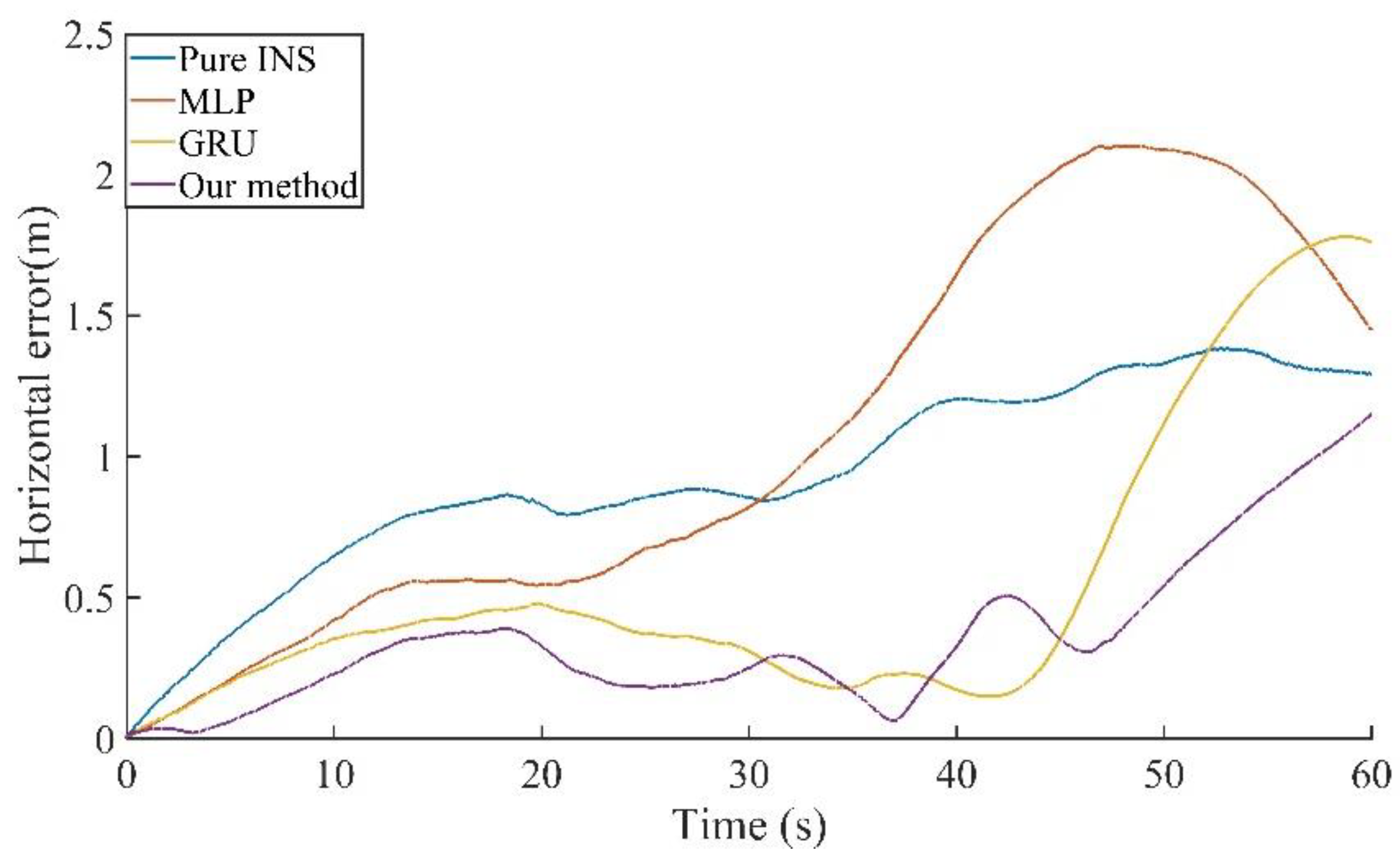
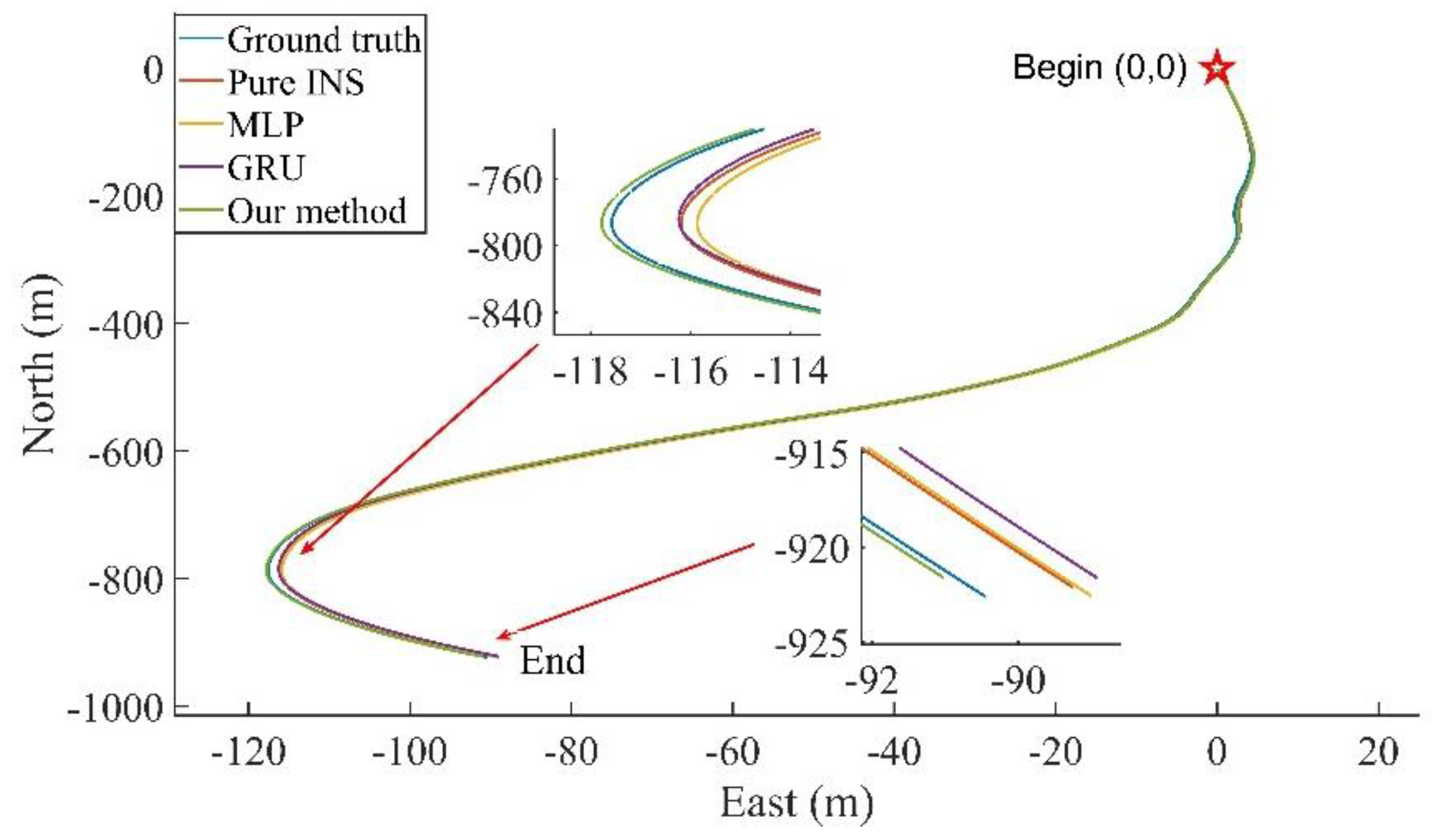
Due to the short GNSS outage time in the first period, the INS that is based on high precision fiber optic gyro shows high accuracy, as shown in Figure 8 and Figure 9, the position errors in the east and north direction during the 60 s GNSS outage are within 2 m. The horizontal direction error of 60 s outage is shown in Figure 10. It can be seen that when the horizontal error is at its maximum, its east and north errors are not necessarily the maximum. Due to the high accuracy of INS, the overall horizontal error is within 2 m, and the difference between the accuracy of different algorithms is not significant, and the turning point of error dispersion mainly occurs at the vehicle corners. The trajectories during this period are shown in the Figure 11, and it can be seen that the position errors are mainly generated at the corners. The maximum position errors are shown in

Table 2. Maximum position error of 60 s outage of Experiment 1.

	East Error (m)	North Error (m)	Horizontal Error (m)
Pure INS	1.38	0.96	1.38
MLP	1.74	1.86	2.10
GRU	1.56	0.89	1.78
Our method	0.57	1.00	1.15

. The proposed method in our paper reduces the maximum position error in the east direction by 58.61%, 67.05%, and 63.35% compared to pure INS, MLP, and GRU, respectively. The maximum position error in the north direction is similar, increasing by 4.44% and 12.74% compared to pure INS and GRU, reducing by 46.34% compared to MLP, and the maximum position in the horizontal direction error is reduced by 16.86%, 45.29%, and 35.34% compared to pure INS, MLP, and GRU, respectively. It can be seen that the accuracy of the RNN is significantly better than that of the MLP.

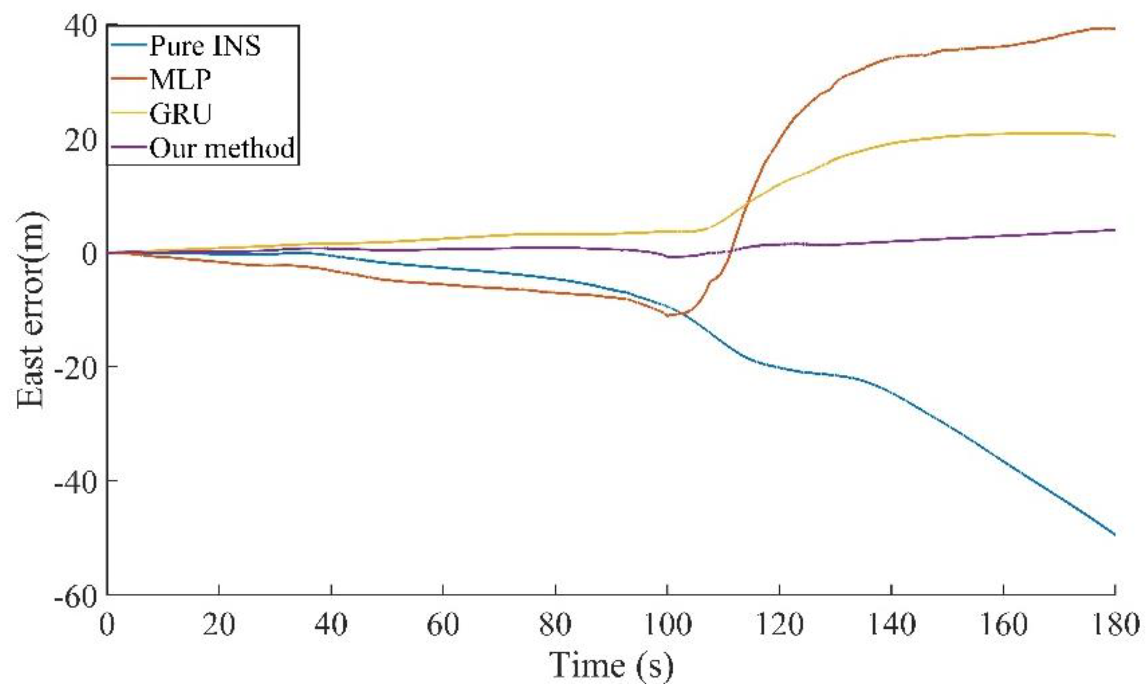
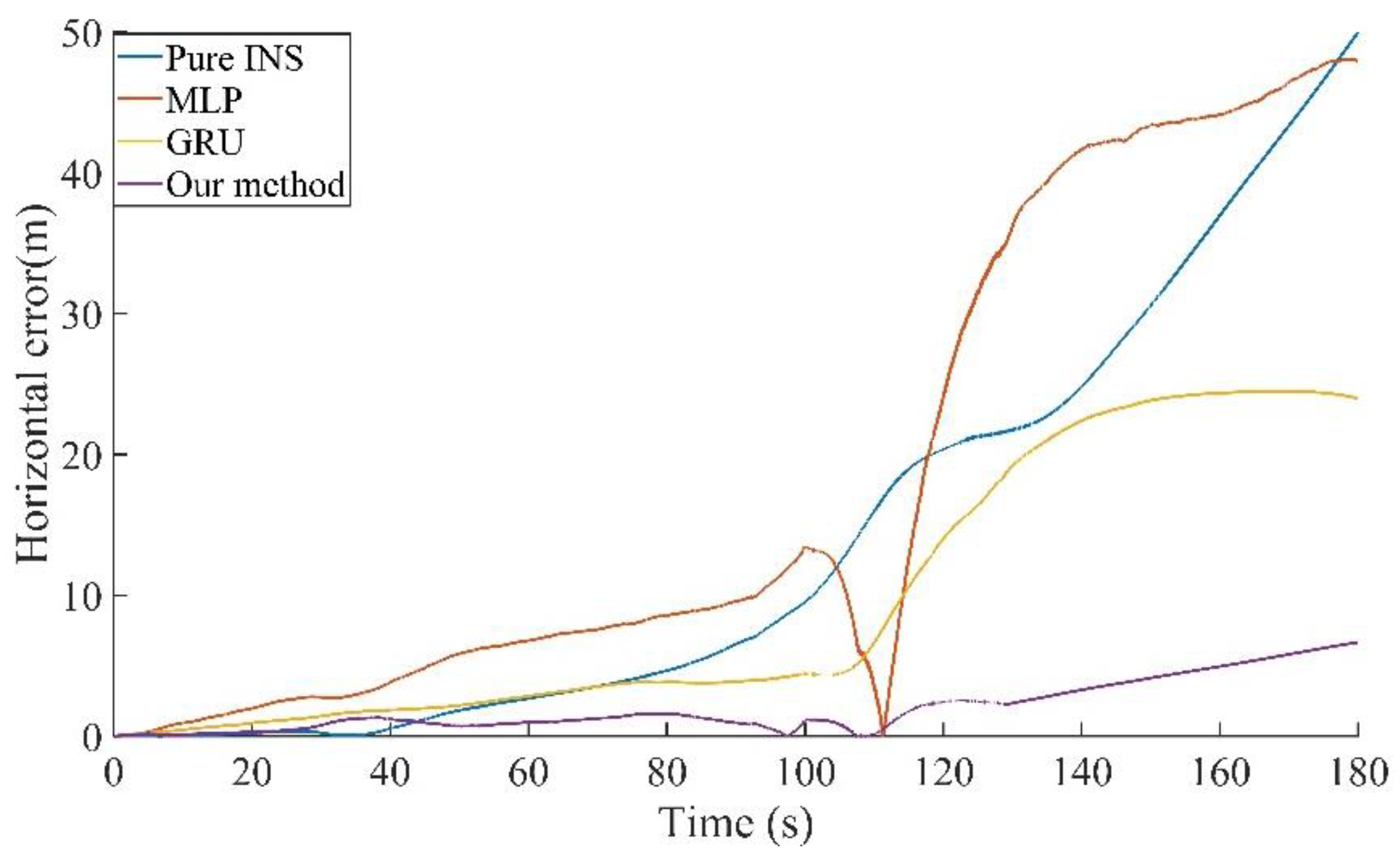
Figure 12 and Figure 13 show the position errors of the different algorithms in the east and north directions during the 120 s GNSS outage. It can be seen that the north position error of the pure INS has started to decrease. The horizontal direction error of 180 s outage is shown in Figure 14, and it can be seen that as the GNSS outage time increases to 3 min, the accuracy of the pure INS starts to dissipate, and the MLP method does not perform well, starting to dissipate from around 100 s. The trajectories during this period are shown in Figure 15. The maximum position errors are shown in

Table 3. Maximum position error of 180 s outage of Experiment 1.

	East Error (m)	North Error (m)	Horizontal Error (m)
Pure INS	49.42	8.58	50.03
MLP	39.35	27.49	47.93
GRU	20.92	12.49	23.98
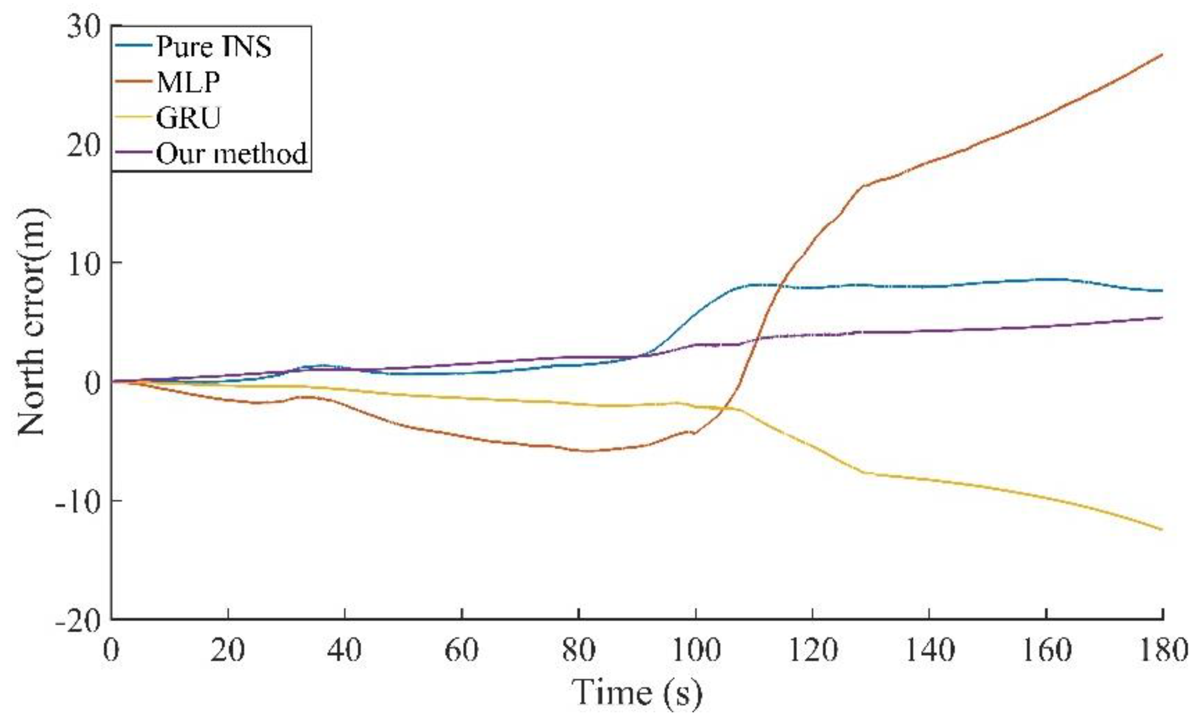
Our method	3.95	5.37	6.67

. Compared to the pure INS, MLP, and GRU, the proposed method in this paper reduces the maximum position errors in the east direction by 92.00%, 89.95%, and 81.10%, in the north direction by 37.39%, 80.45%, and 56.96%, and in the horizontal direction by 86.66%, 86.08%, and 72.18%.

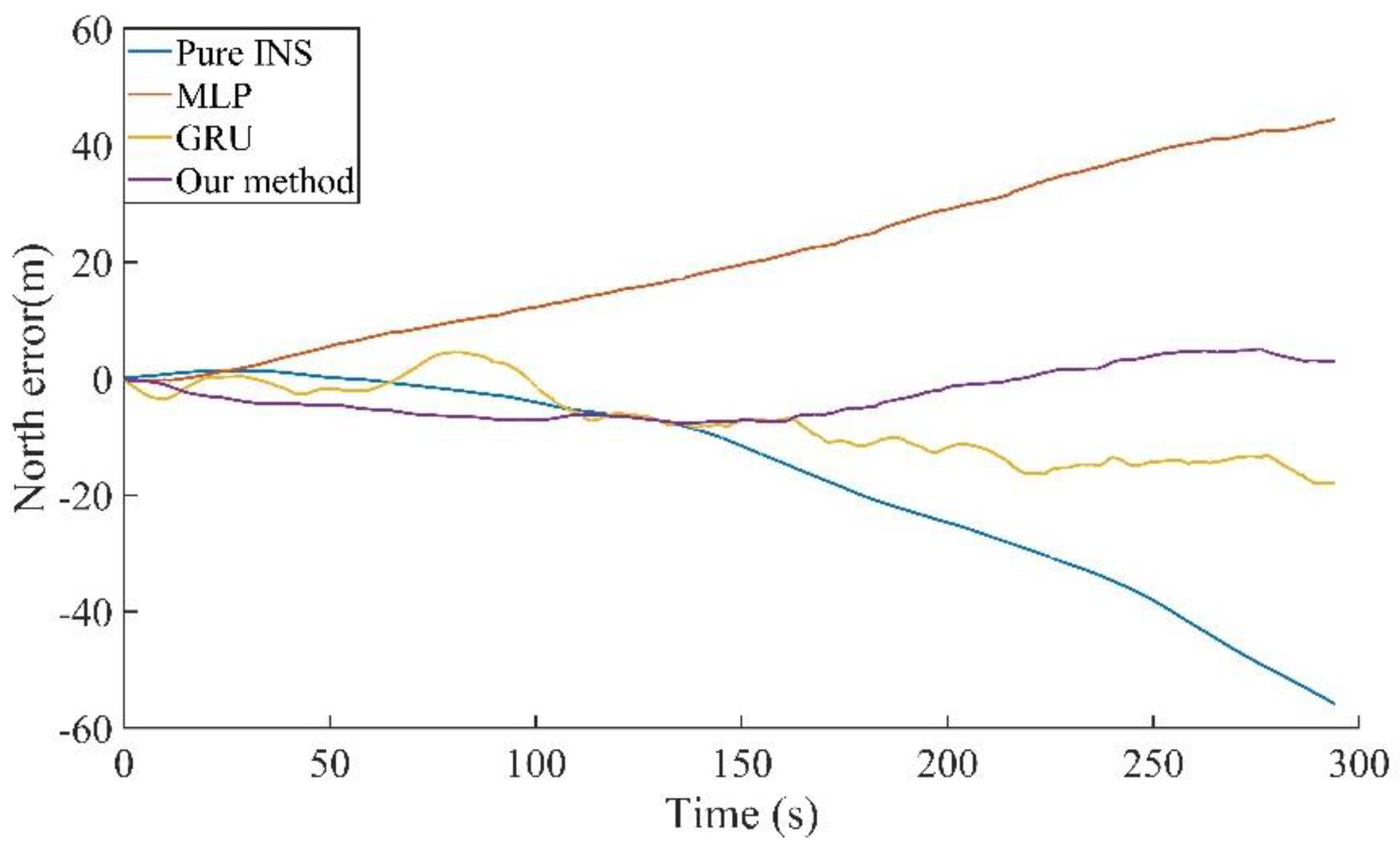
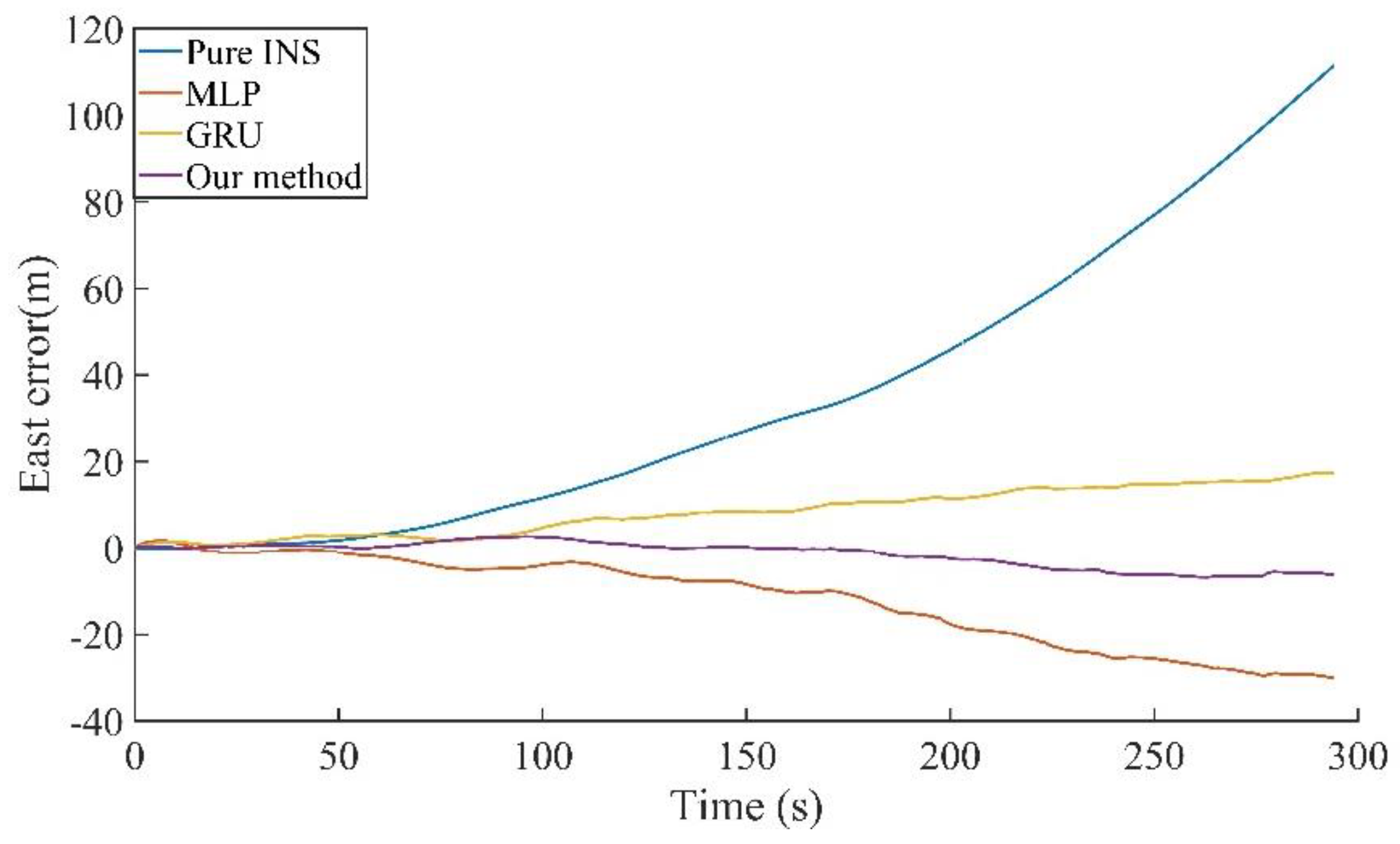
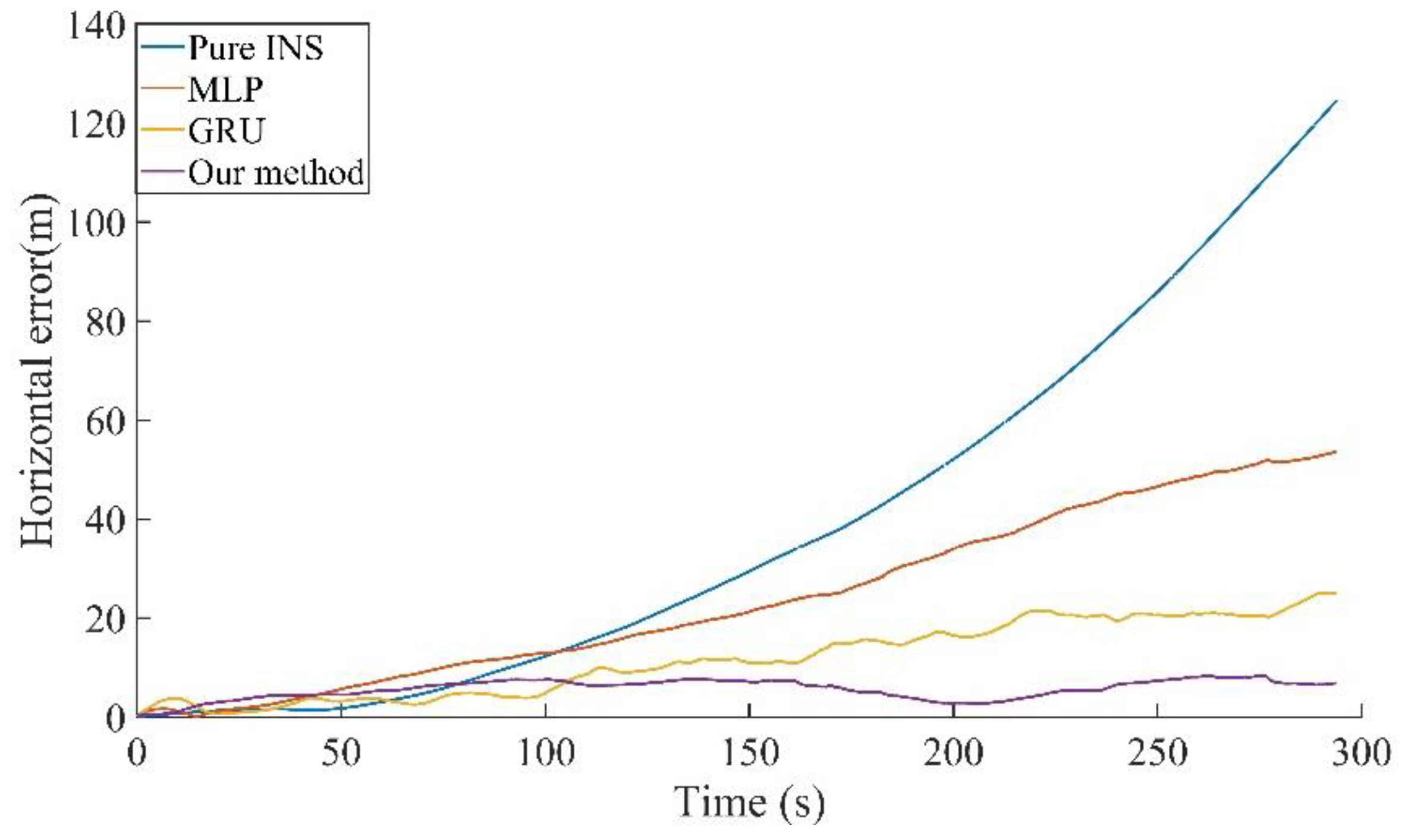
Since the GNSS outage time reached 300 s, the model was switched to the fine model when the GNSS outage time increase to more than two minutes. Figure 16 and Figure 17 show the position errors of the different algorithms in the east and north directions during the 300 s GNSS outage. It can be seen that the prediction performance of MLP for the north position error was unsatisfactory, while the effect of the direction that was proposed in our paper is obvious. 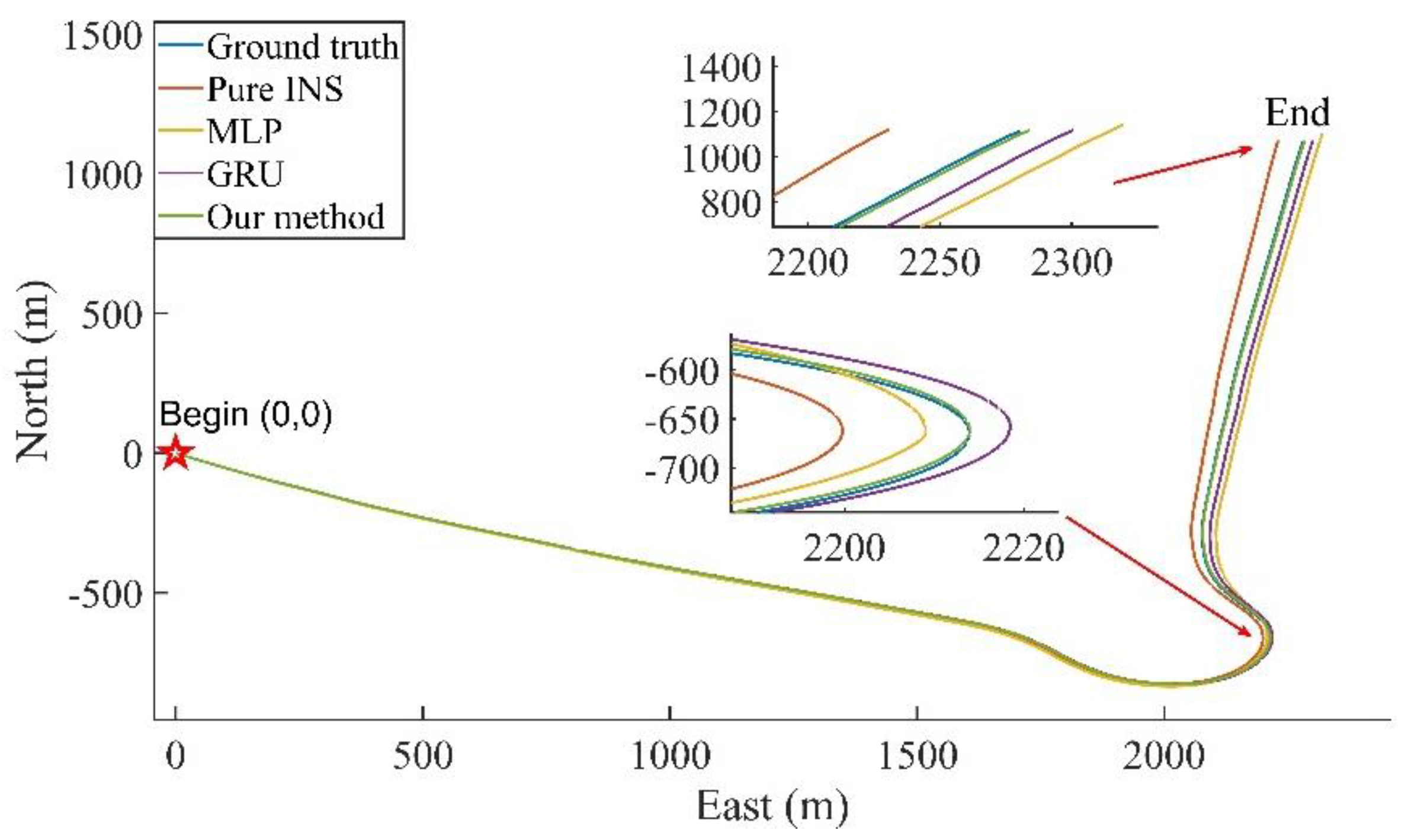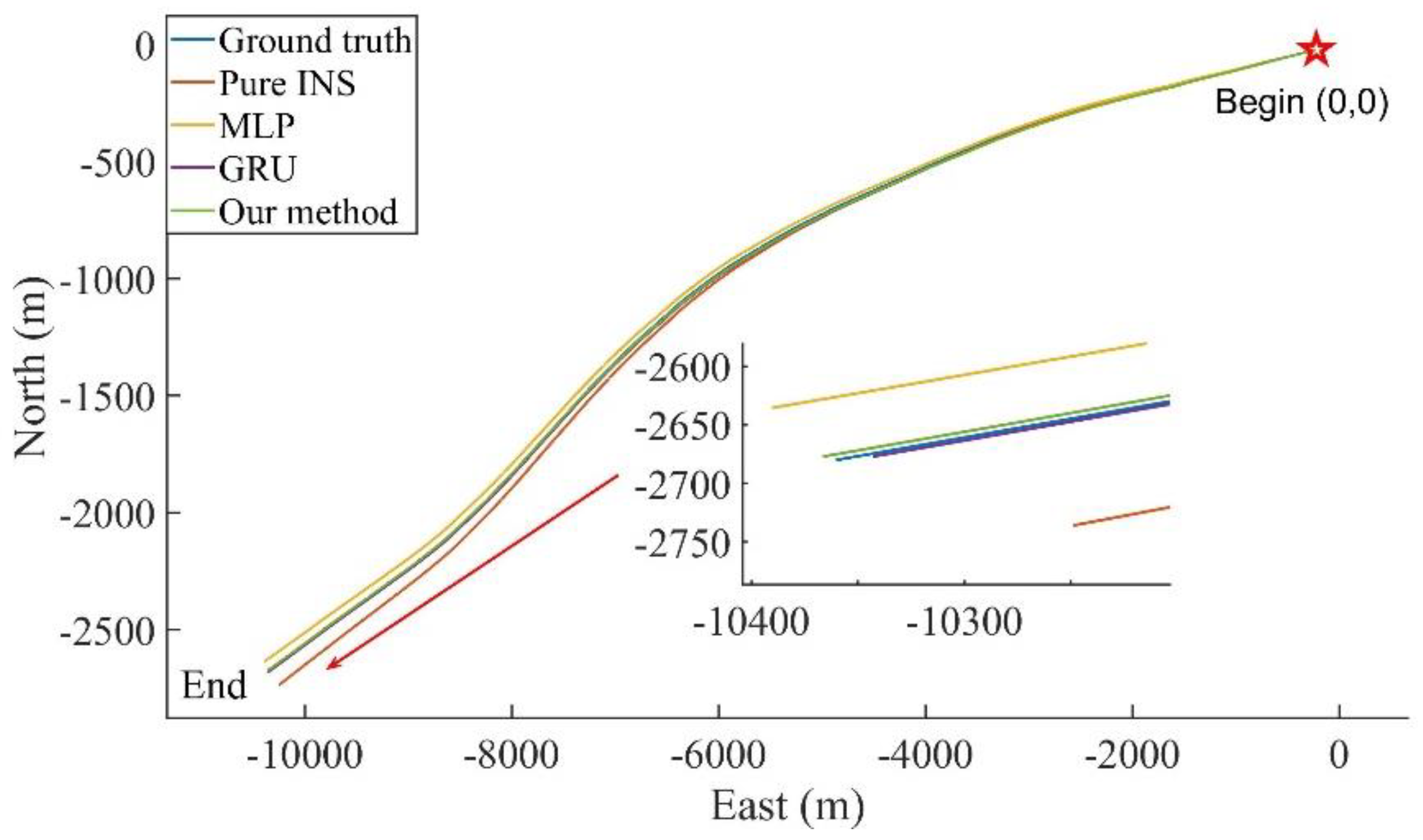Horizontal direction error of 300 s outage is shown in Figure 18. It can be seen that as the GNSS outage time increases to 5 min, the accuracy of both the pure INS and the MLP method begin to diverge, while the GRU and CNN-GRU accuracy is better maintained. The trajectories during this period are shown in the Figure 19. The trajectory that is predicted by the method that is proposed in our paper is close to the real trajectory. The maximum position errors are shown in

Table 4. Maximum position error of 300 s outage of Experiment 1.

	East Error (m)	North Error (m)	Horizontal Error (m)
Pure INS	111.48	55.81	124.67
MLP	30.08	44.51	53.72
GRU	17.40	18.01	24.96
Our method	6.74	7.62	8.28

. Compared to the pure INS, MLP, and GRU, the proposed method in our paper reduces the maximum position errors in the east direction by 93.96%, 77.60%, and 61.27%, in the north direction by 86.34%, 82.87%, and 57.67%, and in the horizontal direction by 93.36%, 84.58%, and 66.81%.

As shown in Figure 20, Experiment 2 contains five tunnels, with lengths of 1.3 km, 1.7 km, 3.2 km, 5.2 km, and 1.7 km, respectively. The first three sections of the tunnel are closely spaced which is specifically designed to more accurately show the algorithms’ effectiveness. As shown in Figure 21, the compensation effect of different algorithms for the first three tunnel sections can be seen. Since RTK cannot obtain position information in the tunnel, we choose the horizontal position error at the end of the tunnel as the evaluation index, and the results are shown in

Table 5. Horizontal position error at the end of the different tunnels.

	#1 (m)	#2 (m)	#3 (m)	#4 (m)	#5 (m)
Pure INS	2.56	5.27	6.82	18.91	6.57
MLP	7.46	6.94	5.77	9.62	4.12
GRU	3.96	5.82	3.49	5.52	2.65
Our method	1.90	3.02	2.52	4.36	1.81

. Compared with pure INS, MLP, and GRU, the method that was proposed in this paper reduces the average horizontal position error at the end of the tunnel by 66.07%, 59.85%, and 36.50%.

5. Conclusions

In order to improve the positioning accuracy of integrated INS/GNSS navigation during GNSS outage, our paper proposes a new AI-assisted method. The method consists of two parts: first, CKF is used to provide more accurate positioning results. Then, by building a CNN-GRU network we can predict the position increments during GNSS outage. In the process, the CNN is utilized to quickly extract the multi-dimensional sequence features, and GRU is used to model the time series. In addition, a new real-time training strategy is proposed for practical application scenarios, where the duration of the GNSS outage time and the motion state information of the vehicle are taken into account in the training strategy. The experimental results show that compared with pure INS, MLP, and GRU, the proposed method reduces the maximum position error in the horizontal direction by 93.36%, 84.58%, and 66.81% in the 5 min simulated GNSS disruption experiments compared to the pure INS, MLP, and GRU, respectively. In the real GNSS failure scenario, the average horizontal position error at the end of the tunnel using our method is reduced by 66.07%, 59.85%, and 36.50%. The algorithm can provide real-time high-precision navigation results with high efficiency and has a good reduction effect on the error dispersion that is caused by prolonged GNSS failure.