
Beyond Classifiers: Remote Sensing Change Detection with Metric Learning

Abstract
:1. Introduction
- We remove classifiers in change detection networks and propose a strong baseline with modified contrastive loss.
- We improve the contrastive loss with triplet loss by searching for triplet pairs in changed and unchanged regions. We further transfer triplet metric learning to semantic change detection. Since multiple classes are provided, we conduct more triplet pairs. To our knowledge, this is the first time triplet loss has been used in change detection both spatially and temporally.
- Extensive experiments have confirmed the effectiveness of our contrastive loss baseline and triplet loss in binary and semantic change detection.
2. Related Work
2.1. Binary Change Detection
2.1.1. Feature Extraction
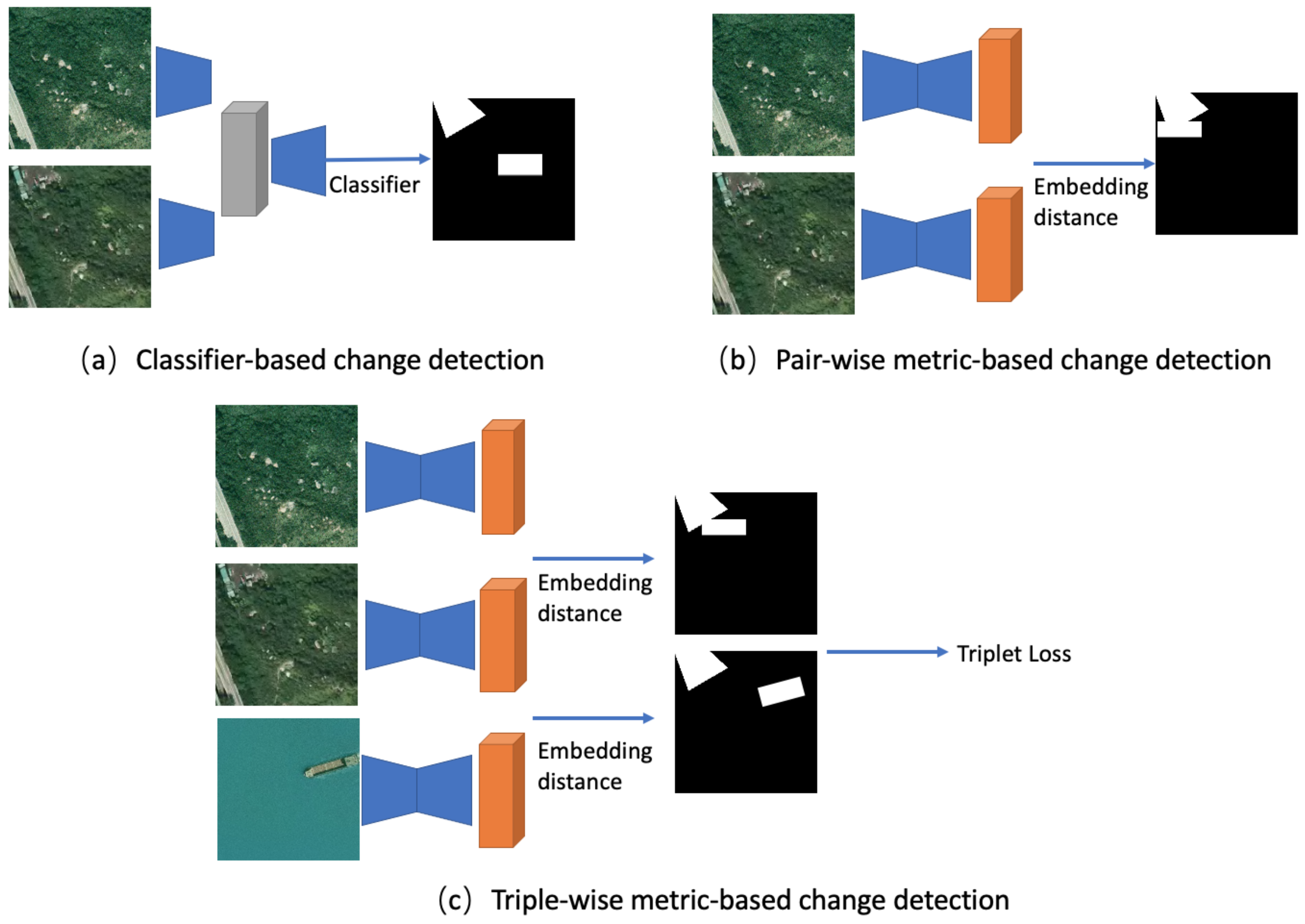
2.1.2. Classifier-Based Methods
2.1.3. Metric-Based Methods
2.1.4. Contrastive Learning Methods
2.2. Semantic Change Detection
2.3. Metric Learning
3. Change Detection by Metric Learning
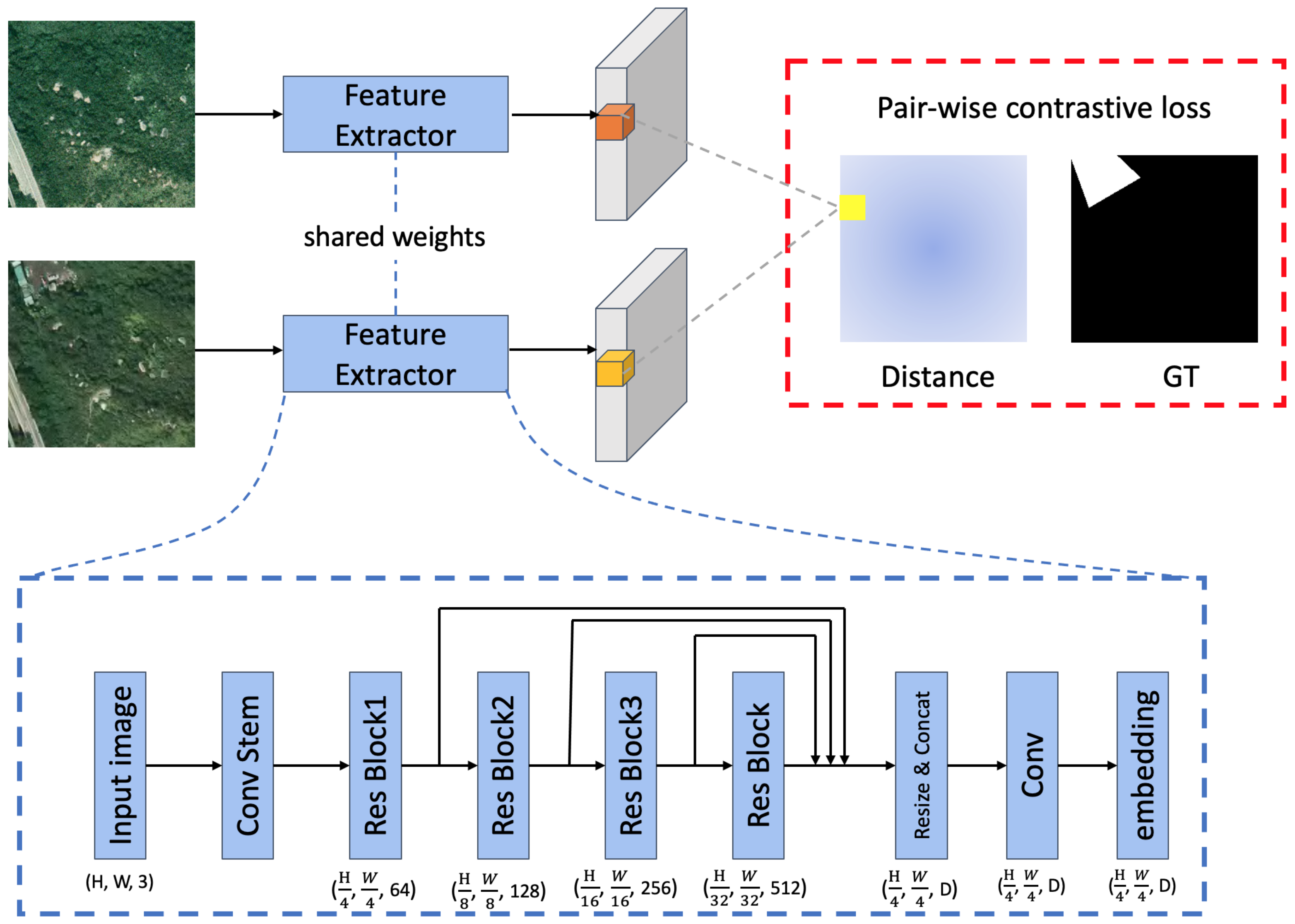
3.1. Framework
3.2. Basic Concept
3.2.1. Definition
3.2.2. Loss Functions
3.3. Contrastive Loss Baseline
3.3.1. Naive Contrastive Loss
3.3.2. Balanced Contrastive Loss
3.3.3. Probability Contrastive Loss
3.3.4. Revert Contrastive Loss
3.3.5. Hard Mining
3.3.6. Overall Loss Function
3.4. Triplet Loss
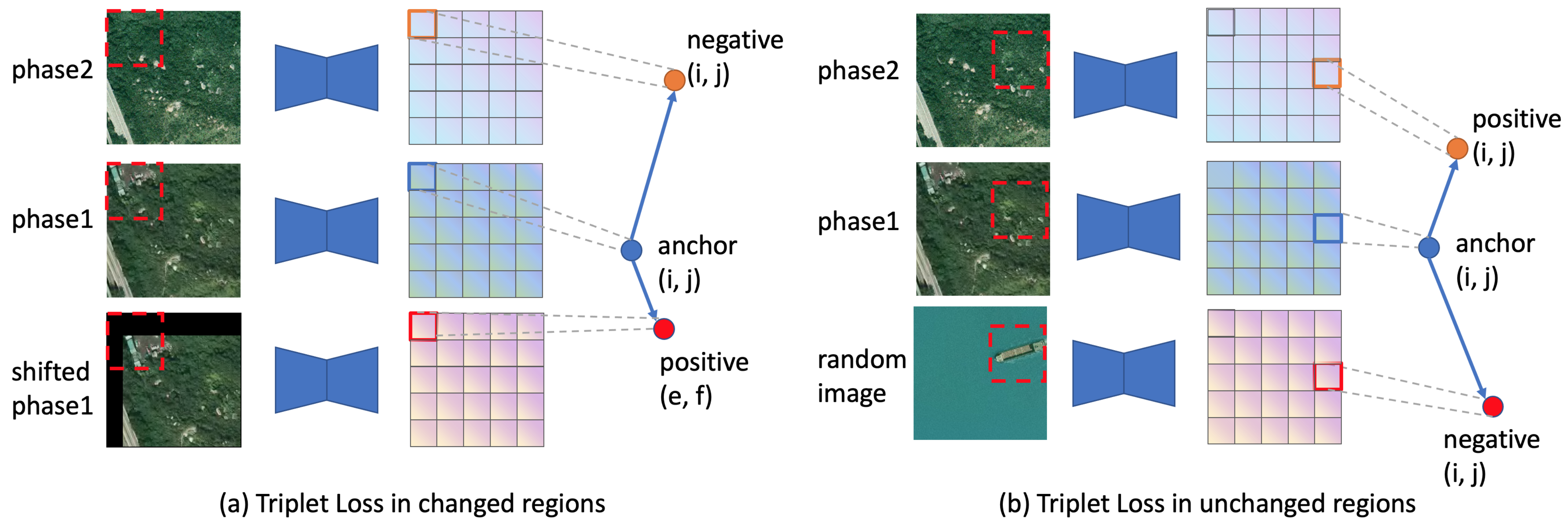
3.4.1. Triplet Loss in Changed Region
- Anchor: pixel embedding at location (i, j) in the changed contour from phase 1.
- Positive: pixel embedding at location (e, f) in the changed contour from phase 1.
- Negative: pixel embedding at location (i, j) in the changed contour from phase 2.

3.4.2. Triplet Loss in Unchanged Region
- Anchor: pixel embedding at location (i, j) in the unchanged region from phase 1.
- Positive: pixel embedding at location (i, j) in the unchanged region from phase 2.
- Negative: pixel embedding at location (i, j) from the random image.
3.4.3. Triplet Pairs in Semantic Change Detection
- Anchor: pixel embedding at location (i, j) in the changed region from phase 1.
- Positive: pixel embedding at location (e, f) in the changed region from phase 1, with the same semantic label as Anchor.
- Negative: pixel embedding at location (u, v) in the changed region from phase 2, with different semantic labels from Anchor.
3.4.4. Overall Loss Function
4. Experiments
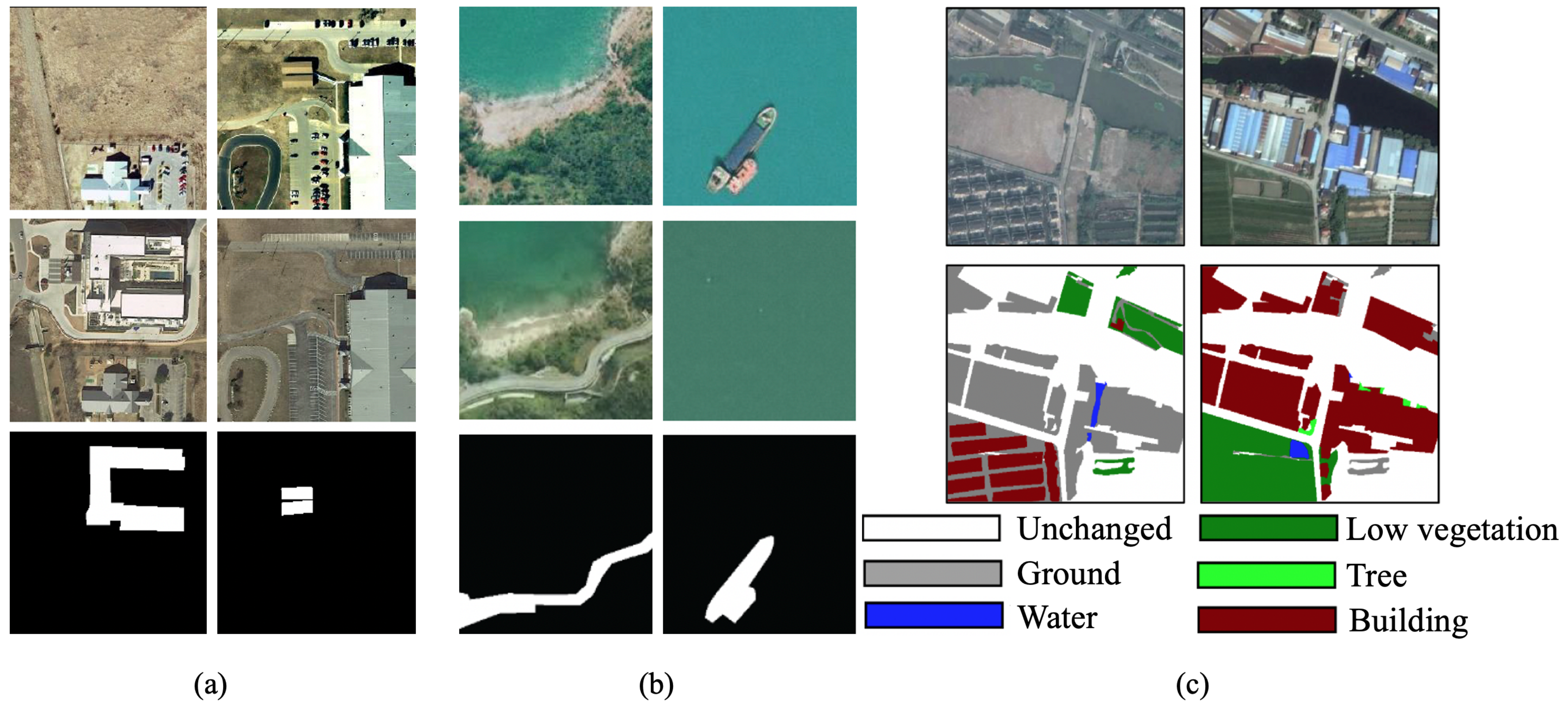
4.1. Datasets
4.2. Implementation Details
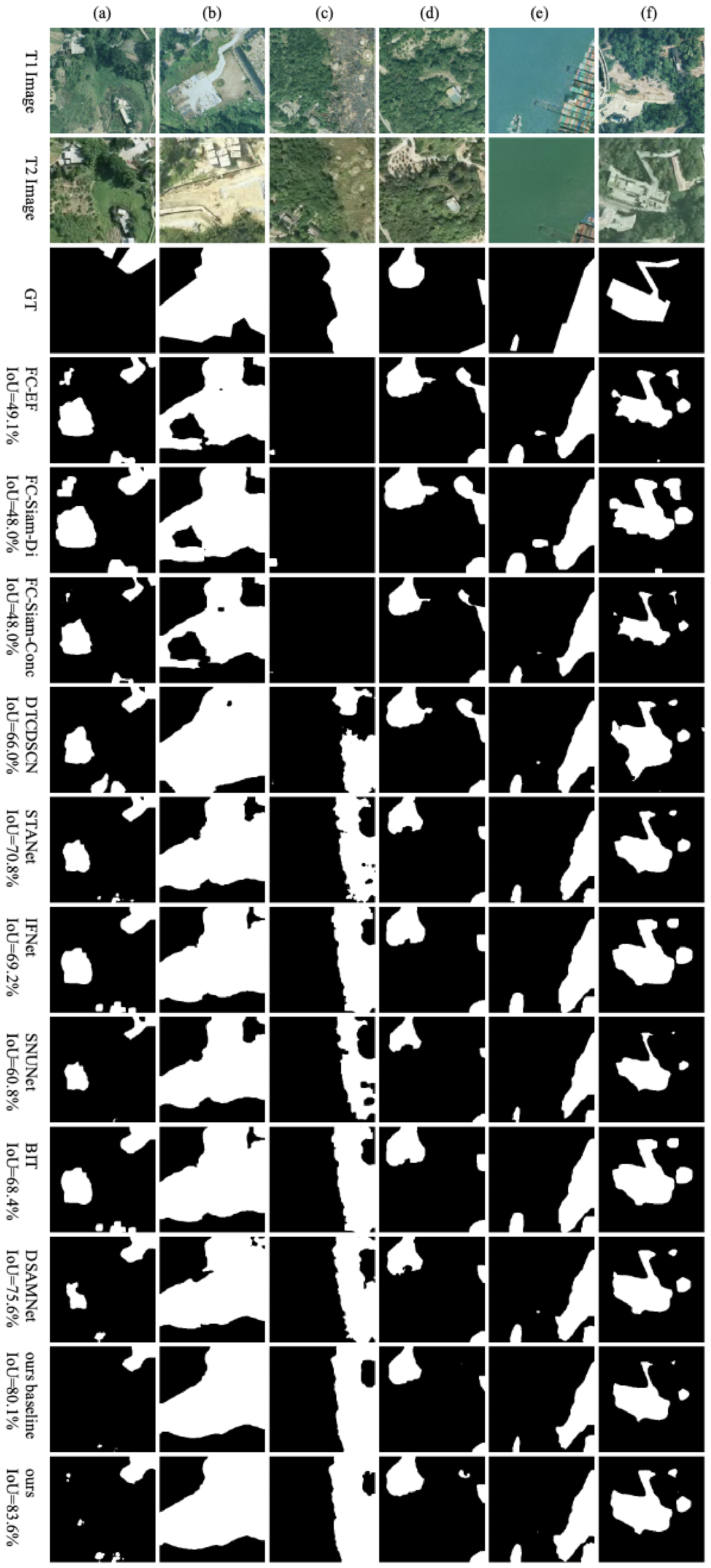
4.3. Binary Change Detection Results
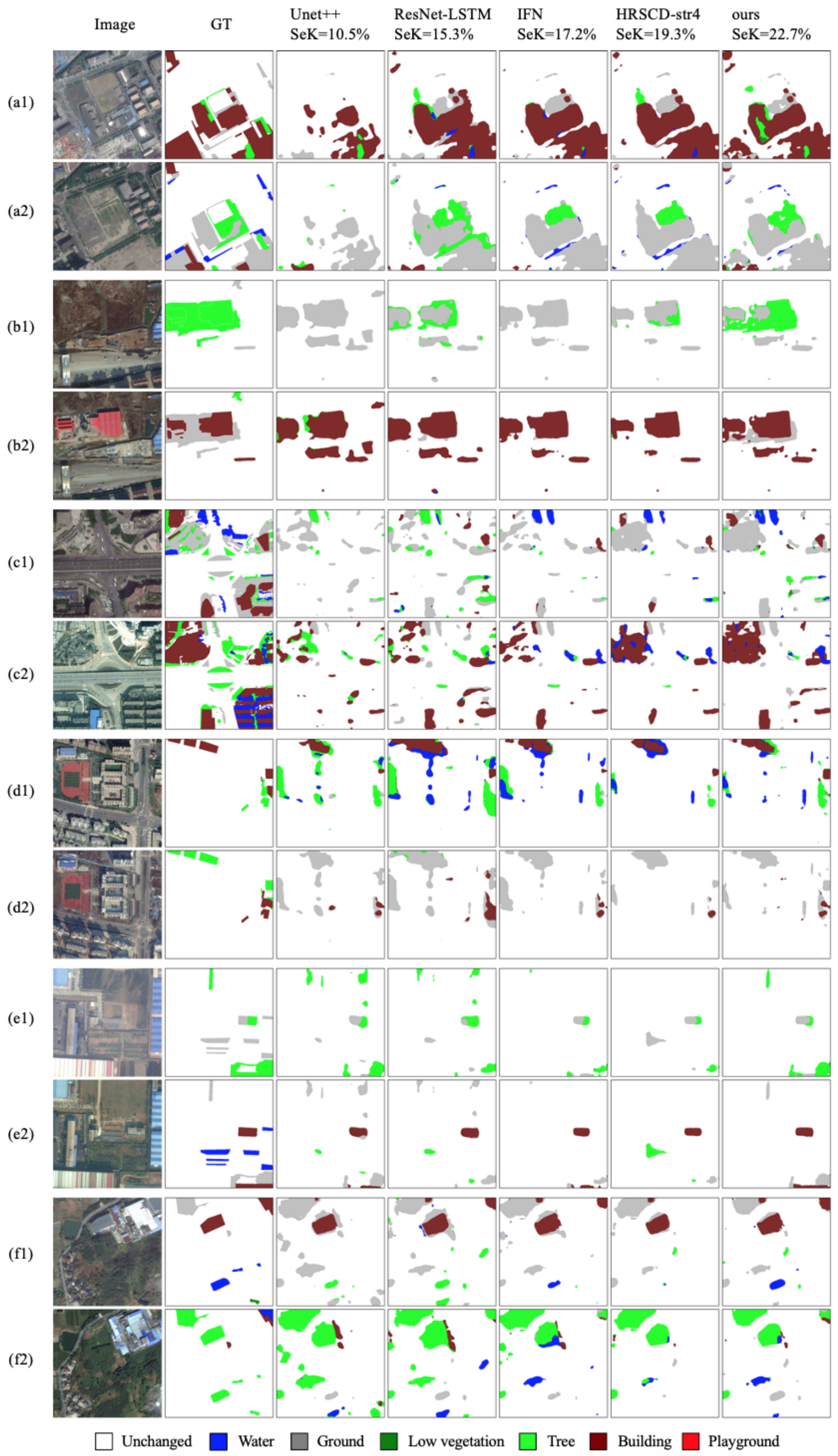
4.4. Semantic Change Detection Results
4.5. Ablation Study
4.5.1. Contrastive Loss Baseline
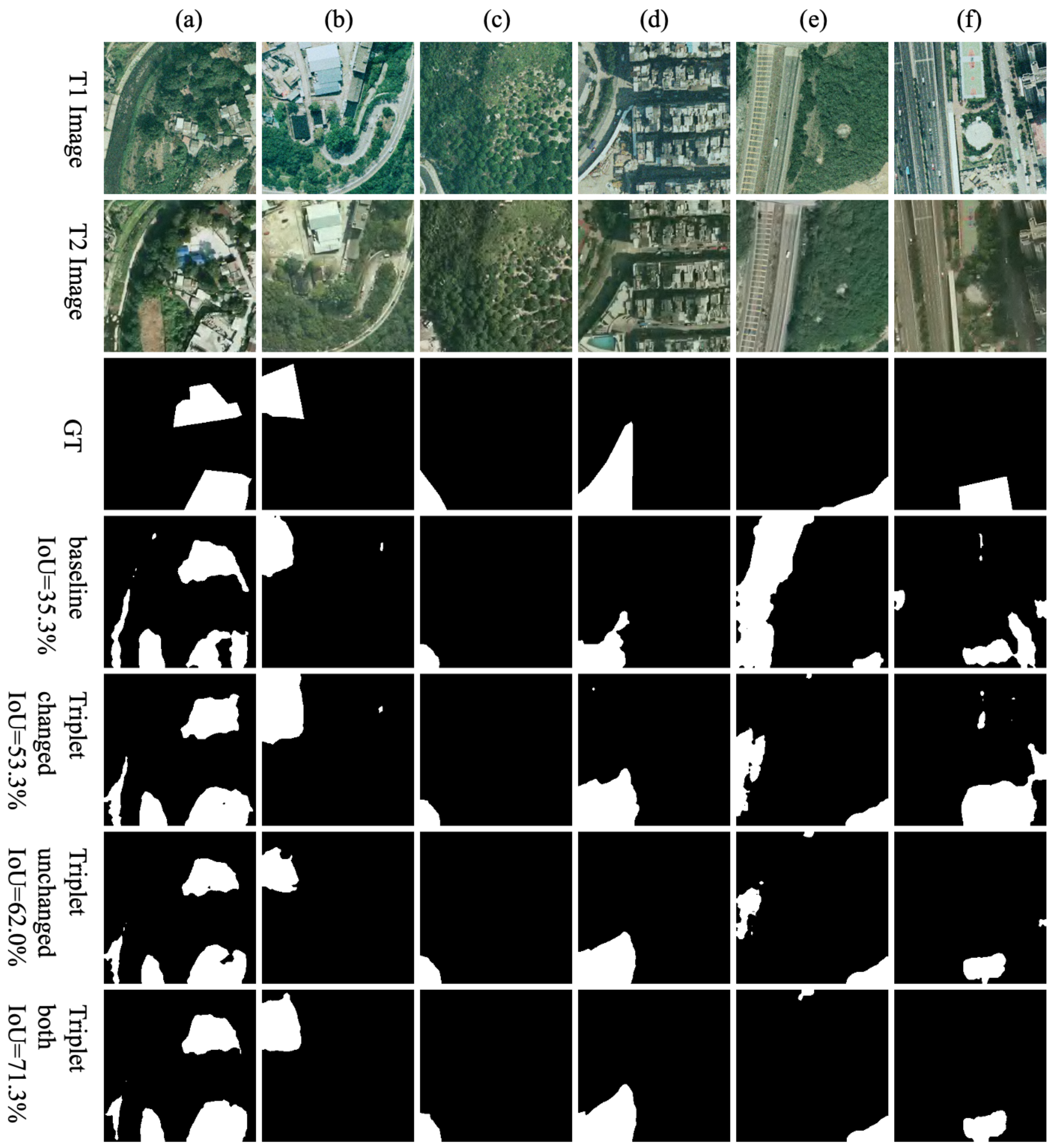
4.5.2. Two Sources of Triplet Pairs
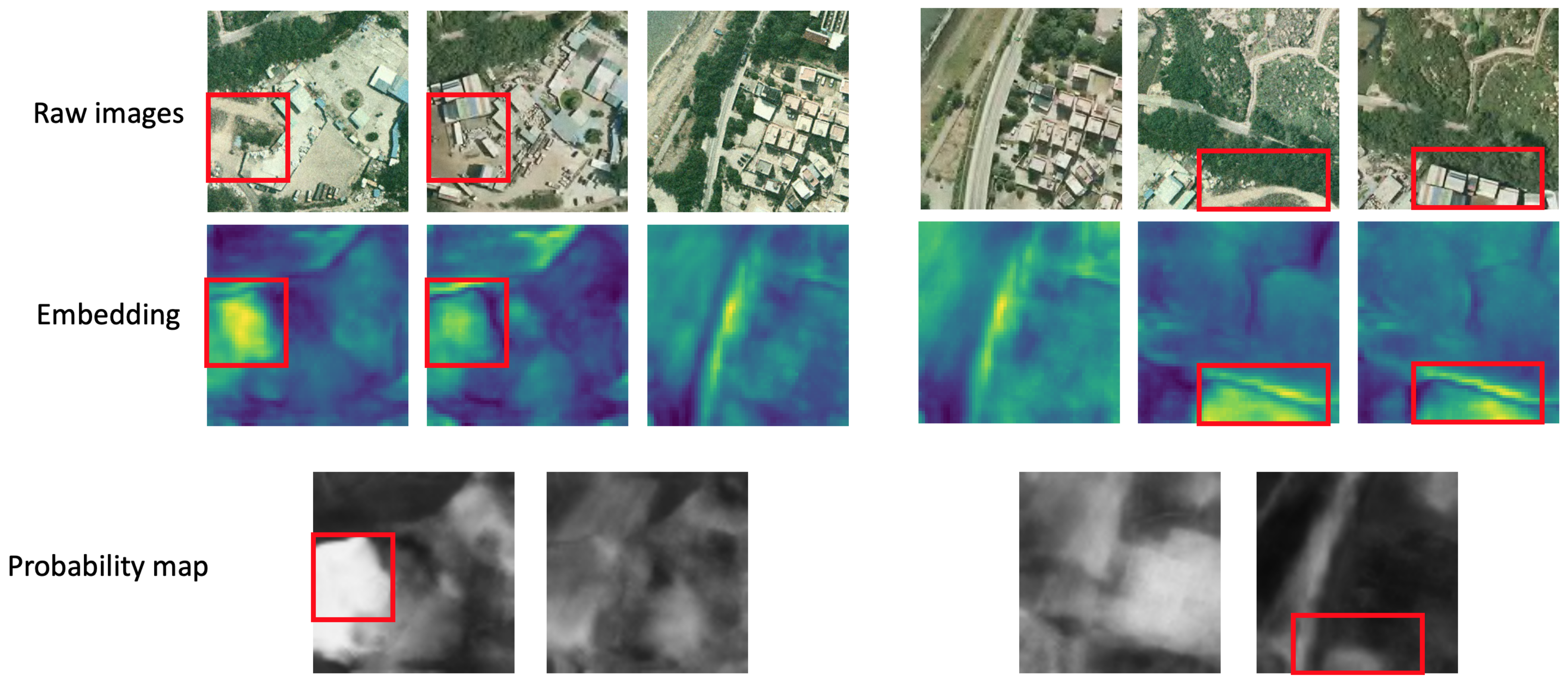
4.5.3. Embedding Visualization
5. Discussion
6. Conclusions
Author Contributions
Funding
Data Availability Statement
Conflicts of Interest
References
- Hussain, M.; Chen, D.; Cheng, A.; Wei, H.; Stanley, D. Change detection from remotely sensed images: From pixel-based to object-based approaches. ISPRS J. Photogramm. Remote Sens. 2013, 80, 91–106. [Google Scholar] [CrossRef]
- Shi, Q.; Liu, M.; Li, S.; Liu, X.; Wang, F.; Zhang, L. A deeply supervised attention metric-based network and an open aerial image dataset for remote sensing change detection. IEEE Trans. Geosci. Remote Sens. 2021, 60, 5604816. [Google Scholar] [CrossRef]
- Mahdavi, S.; Salehi, B.; Huang, W.; Amani, M.; Brisco, B. A PolSAR change detection index based on neighborhood information for flood mapping. Remote Sens. 2019, 11, 1854. [Google Scholar] [CrossRef]
- Woodcock, C.E.; Loveland, T.R.; Herold, M.; Bauer, M.E. Transitioning from change detection to monitoring with remote sensing: A paradigm shift. Remote Sens. Environ. 2020, 238, 111558. [Google Scholar] [CrossRef]
- Daudt, R.C.; Le Saux, B.; Boulch, A. Fully convolutional siamese networks for change detection. In Proceedings of the 2018 25th IEEE International Conference on Image Processing (ICIP), Athens, Greece, 7–10 October 2018; pp. 4063–4067. [Google Scholar]
- Chen, H.; Qi, Z.; Shi, Z. Remote sensing image change detection with transformers. IEEE Trans. Geosci. Remote Sens. 2021, 60, 5607514. [Google Scholar] [CrossRef]
- Chen, H.; Shi, Z. A spatial-temporal attention-based method and a new dataset for remote sensing image change detection. Remote Sens. 2020, 12, 1662. [Google Scholar] [CrossRef]
- Sun, Y.; Fu, K.; Wang, Z.; Zhang, C.; Ye, J. Road Network Metric Learning for Estimated Time of Arrival. In Proceedings of the 2020 25th International Conference On Pattern Recognition (ICPR), Milan, Italy, 10–15 January 2021; pp. 1820–1827. [Google Scholar]
- Hadsell, R.; Chopra, S.; LeCun, Y. Dimensionality reduction by learning an invariant mapping. In Proceedings of the 2006 IEEE Computer Society Conference on Computer Vision and Pattern Recognition (CVPR’06), New York, NY, USA, 17–22 June 2006; Volume 2, pp. 1735–1742. [Google Scholar]
- Schroff, F.; Kalenichenko, D.; Philbin, J. Facenet: A unified embedding for face recognition and clustering. In Proceedings of the IEEE Conference on Computer Vision and Pattern Recognition, Boston, MA, USA, 7–12 June 2015; pp. 815–823. [Google Scholar]
- Huang, G.B.; Mattar, M.; Berg, T.; Learned-Miller, E. Labeled faces in the wild: A database forstudying face recognition in unconstrained environments. In Proceedings of the Workshop on faces in ‘Real-Life’ Images: Detection, Alignment, and Recognition, Tuscany, Italy, 28 July–3 August 2008; Springer: Berlin/Heidelberg, Germany, 2008; p. 1. [Google Scholar]
- Zhang, M.; Xu, G.; Chen, K.; Yan, M.; Sun, X. Triplet-based semantic relation learning for aerial remote sensing image change detection. IEEE Geosci. Remote Sens. Lett. 2018, 16, 266–270. [Google Scholar] [CrossRef]
- Hou, X.; Bai, Y.; Li, Y.; Shang, C.; Shen, Q. High-resolution triplet network with dynamic multiscale feature for change detection on satellite images. ISPRS J. Photogramm. Remote Sens. 2021, 177, 103–115. [Google Scholar] [CrossRef]
- Liu, J.; Gong, M.; Qin, K.; Zhang, P. A deep convolutional coupling network for change detection based on heterogeneous optical and radar images. IEEE Trans. Neural Netw. Learn. Syst. 2016, 29, 545–559. [Google Scholar] [CrossRef]
- Zhan, Y.; Fu, K.; Yan, M.; Sun, X.; Wang, H.; Qiu, X. Change detection based on deep siamese convolutional network for optical aerial images. IEEE Geosci. Remote Sens. Lett. 2017, 14, 1845–1849. [Google Scholar] [CrossRef]
- Wang, M.; Tan, K.; Jia, X.; Wang, X.; Chen, Y. A deep siamese network with hybrid convolutional feature extraction module for change detection based on multi-sensor remote sensing images. Remote Sens. 2020, 12, 205. [Google Scholar] [CrossRef]
- Yang, K.; Xia, G.S.; Liu, Z.; Du, B.; Yang, W.; Pelillo, M. Asymmetric siamese networks for semantic change detection. arXiv 2020, arXiv:2010.05687. [Google Scholar]
- Khelifi, L.; Mignotte, M. Deep Learning for Change Detection in Remote Sensing Images: Comprehensive Review and Meta-Analysis. IEEE Access 2020, 8, 126385–126400. [Google Scholar] [CrossRef]
- Ji, S.; Wei, S.; Lu, M. Fully convolutional networks for multisource building extraction from an open aerial and satellite imagery data set. IEEE Trans. Geosci. Remote Sens. 2018, 57, 574–586. [Google Scholar] [CrossRef]
- Zhang, W.; Lu, X. The Spectral-Spatial Joint Learning for Change Detection in Multispectral Imagery. Remote Sens. 2019, 11, 240. [Google Scholar] [CrossRef]
- Song, A.; Choi, J.; Han, Y.; Kim, Y. Change detection in hyperspectral images using recurrent 3D fully convolutional networks. Remote Sens. 2018, 10, 1827. [Google Scholar] [CrossRef]
- Liu, M.; Shi, Q.; Marinoni, A.; He, D.; Liu, X.; Zhang, L. Super-resolution-based change detection network with stacked attention module for images with different resolutions. IEEE Trans. Geosci. Remote Sens. 2021, 60, 4403718. [Google Scholar] [CrossRef]
- Mou, L.; Bruzzone, L.; Zhu, X.X. Learning spectral-spatial-temporal features via a recurrent convolutional neural network for change detection in multispectral imagery. IEEE Trans. Geosci. Remote Sens. 2018, 57, 924–935. [Google Scholar] [CrossRef]
- Luppino, L.T.; Kampffmeyer, M.; Bianchi, F.M.; Moser, G.; Serpico, S.B.; Jenssen, R.; Anfinsen, S.N. Deep image translation with an affinity-based change prior for unsupervised multimodal change detection. IEEE Trans. Geosci. Remote Sens. 2021, 60, 4700422. [Google Scholar] [CrossRef]
- Li, X.; Du, Z.; Huang, Y.; Tan, Z. A deep translation (GAN) based change detection network for optical and SAR remote sensing images. ISPRS J. Photogramm. Remote Sens. 2021, 179, 14–34. [Google Scholar] [CrossRef]
- Sun, Y.; Lei, L.; Li, X.; Sun, H.; Kuang, G. Nonlocal patch similarity based heterogeneous remote sensing change detection. Pattern Recognit. 2021, 109, 107598. [Google Scholar] [CrossRef]
- Peng, D.; Zhang, Y.; Guan, H. End-to-end change detection for high resolution satellite images using improved UNet++. Remote Sens. 2019, 11, 1382. [Google Scholar] [CrossRef]
- Zhang, C.; Yue, P.; Tapete, D.; Jiang, L.; Shangguan, B.; Huang, L.; Liu, G. A deeply supervised image fusion network for change detection in high resolution bi-temporal remote sensing images. ISPRS J. Photogramm. Remote Sens. 2020, 166, 183–200. [Google Scholar] [CrossRef]
- Zhang, M.; Shi, W. A feature difference convolutional neural network-based change detection method. IEEE Trans. Geosci. Remote Sens. 2020, 58, 7232–7246. [Google Scholar] [CrossRef]
- Zhao, W.; Mou, L.; Chen, J.; Bo, Y.; Emery, W.J. Incorporating Metric Learning and Adversarial Network for Seasonal Invariant Change Detection. IEEE Trans. Geosci. Remote Sens. 2020, 58, 2720–2731. [Google Scholar] [CrossRef]
- Bandara, W.G.C.; Patel, V.M. A Transformer-Based Siamese Network for Change Detection. arXiv 2012, arXiv:2201.01293. [Google Scholar]
- Hou, B.; Wang, Y.; Liu, Q. Change detection based on deep features and low rank. IEEE Geosci. Remote Sens. Lett. 2017, 14, 2418–2422. [Google Scholar] [CrossRef]
- Saha, S.; Bovolo, F.; Bruzzone, L. Unsupervised deep change vector analysis for multiple-change detection in VHR images. IEEE Trans. Geosci. Remote Sens. 2019, 57, 3677–3693. [Google Scholar] [CrossRef]
- Saha, S.; Bovolo, F.; Bruzzone, L. Building change detection in VHR SAR images via unsupervised deep transcoding. IEEE Trans. Geosci. Remote Sens. 2020, 59, 1917–1929. [Google Scholar] [CrossRef]
- Zheng, Z.; Ma, A.; Zhang, L.; Zhong, Y. Change is Everywhere: Single-Temporal Supervised Object Change Detection in Remote Sensing Imagery. In Proceedings of the IEEE/CVF International Conference on Computer Vision, Montreal, QC, Canada, 10–17 October 2021; pp. 15193–15202. [Google Scholar]
- Akiva, P.; Purri, M.; Leotta, M. Self-Supervised Material and Texture Representation Learning for Remote Sensing Tasks. arXiv 2021, arXiv:2112.01715. [Google Scholar]
- Chen, Y.; Bruzzone, L. Self-supervised Remote Sensing Images Change Detection at Pixel-level. arXiv 2021, arXiv:2105.08501. [Google Scholar]
- Chen, H.; Zao, Y.; Liu, L.; Chen, S.; Shi, Z. Semantic decoupled representation learning for remote sensing image change detection. arXiv 2022, arXiv:2201.05778. [Google Scholar]
- Wu, C.; Du, B.; Zhang, L. Fully Convolutional Change Detection Framework with Generative Adversarial Network for Unsupervised, Weakly Supervised and Regional Supervised Change Detection. arXiv 2022, arXiv:2201.06030. [Google Scholar]
- Bruzzone, L.; Serpico, S.B. An iterative technique for the detection of land-cover transitions in multitemporal remote-sensing images. IEEE Trans. Geosci. Remote Sens. 1997, 35, 858–867. [Google Scholar] [CrossRef]
- Liu, S.; Bruzzone, L.; Bovolo, F.; Zanetti, M.; Du, P. Sequential spectral change vector analysis for iteratively discovering and detecting multiple changes in hyperspectral images. IEEE Trans. Geosci. Remote Sens. 2015, 53, 4363–4378. [Google Scholar] [CrossRef]
- Daudt, R.C.; Le Saux, B.; Boulch, A.; Gousseau, Y. Multitask learning for large-scale semantic change detection. Comput. Vis. Image Underst. 2019, 187, 102783. [Google Scholar] [CrossRef] [Green Version]
- Ding, L.; Guo, H.; Liu, S.; Mou, L.; Zhang, J.; Bruzzone, L. Bi-Temporal Semantic Reasoning for the Semantic Change Detection in HR Remote Sensing Images. arXiv 2021, arXiv:2108.06103. [Google Scholar] [CrossRef]
- Wang, Y.; Zhang, Y.; Zhang, F.; Wang, S.; Lin, M.; Zhang, Y.; Sun, X. Ada-nets: Face clustering via adaptive neighbour discovery in the structure space. arXiv 2022, arXiv:2202.03800. [Google Scholar]
- Zhang, Y.; Huang, Y.; Wang, L.; Yu, S. A comprehensive study on gait biometrics using a joint CNN-based method. Pattern Recognit. 2019, 93, 228–236. [Google Scholar] [CrossRef]
- Luo, H.; Gu, Y.; Liao, X.; Lai, S.; Jiang, W. Bag of tricks and a strong baseline for deep person re-identification. In Proceedings of the IEEE Conference on Computer Vision and Pattern Recognition Workshops, Long Beach, CA, USA, 16–17 June 2019. [Google Scholar]
- Zhang, Y.; Qian, Q.; Liu, C.; Chen, W.; Wang, F.; Li, H.; Jin, R. Graph convolution for re-ranking in person re-identification. In Proceedings of the ICASSP 2022—2022 IEEE International Conference on Acoustics, Speech and Signal Processing (ICASSP), Singapore, 23–27 May 2022; pp. 2704–2708. [Google Scholar]
- Zhang, Y.; Liu, C.; Chen, W.; Xu, X.; Wang, F.; Li, H.; Hu, S.; Zhao, X. Revisiting instance search: A new benchmark using Cycle Self-Training. Neurocomputing 2022, 501, 270–284. [Google Scholar] [CrossRef]
- He, S.; Luo, H.; Chen, W.; Zhang, M.; Zhang, Y.; Wang, F.; Li, H.; Jiang, W. Multi-domain learning and identity mining for vehicle re-identification. In Proceedings of the IEEE/CVF Conference on Computer Vision and Pattern Recognition Workshops, Seattle, WA, USA, 14–19 June 2020; pp. 582–583. [Google Scholar]
- Liu, C.; Zhang, Y.; Luo, H.; Tang, J.; Chen, W.; Xu, X.; Wang, F.; Li, H.; Shen, Y.D. City-scale multi-camera vehicle tracking guided by crossroad zones. In Proceedings of the IEEE/CVF Conference on Computer Vision and Pattern Recognition, Nashville, TN, USA, 19–25 June 2021; pp. 4129–4137. [Google Scholar]
- Luo, H.; Chen, W.; Xu, X.; Gu, J.; Zhang, Y.; Liu, C.; Jiang, Y.; He, S.; Wang, F.; Li, H. An empirical study of vehicle re-identification on the AI City Challenge. In Proceedings of the IEEE/CVF Conference on Computer Vision and Pattern Recognition, Nashville, TN, USA, 19–25 June 2021; pp. 4095–4102. [Google Scholar]
- Liu, C.; Zhang, Y.; Chen, W.; Wang, F.; Li, H.; Shen, Y.D. Adaptive Matching Strategy for Multi-Target Multi-Camera Tracking. In Proceedings of the ICASSP 2022—2022 IEEE International Conference on Acoustics, Speech and Signal Processing (ICASSP), Singapore, 23–27 May 2022; pp. 2934–2938. [Google Scholar]
- Zhang, Y.; Huang, Y.; Wang, L. Multi-task deep learning for fast online multiple object tracking. In Proceedings of the 2017 4th IAPR Asian Conference on Pattern Recognition (ACPR), Nanjing, China, 26–29 November 2017; pp. 138–143. [Google Scholar]
- Du, F.; Xu, B.; Tang, J.; Zhang, Y.; Wang, F.; Li, H. 1st place solution to eccv-tao-2020: Detect and represent any object for tracking. arXiv 2021, arXiv:2101.08040. [Google Scholar]
- Zhang, Y.; Huang, Y.; Wang, L. What makes for good multiple object trackers? In Proceedings of the 2016 IEEE International Conference on Digital Signal Processing (DSP), Beijing, China, 16–18 October 2016; pp. 467–471. [Google Scholar]
- Yuqi, Z.; Xianzhe, X.; Weihua, C.; Yaohua, W.; Fangyi, Z.; Fan, W.; Hao, L. 2nd Place Solution to Google Landmark Retrieval 2021. arXiv 2021, arXiv:2110.04294. [Google Scholar]
- Wen, Y.; Zhang, K.; Li, Z.; Qiao, Y. A discriminative feature learning approach for deep face recognition. In Proceedings of the European Conference on Computer Vision, Amsterdam, The Netherlands, 11–14 October 2016; Springer: Cham, Switzerland, 2016; pp. 499–515. [Google Scholar]
- Liu, W.; Wen, Y.; Yu, Z.; Li, M.; Raj, B.; Song, L. Sphereface: Deep hypersphere embedding for face recognition. In Proceedings of the IEEE Conference on Computer Vision and Pattern Recognition, Honolulu, HI, USA, 21–26 July 2017; pp. 212–220. [Google Scholar]
- Wang, H.; Wang, Y.; Zhou, Z.; Ji, X.; Gong, D.; Zhou, J.; Li, Z.; Liu, W. Cosface: Large margin cosine loss for deep face recognition. In Proceedings of the IEEE Conference on Computer Vision and Pattern Recognition, Salt Lake City, UT, USA, 18–23 June 2018; pp. 5265–5274. [Google Scholar]
- Deng, J.; Guo, J.; Xue, N.; Zafeiriou, S. Arcface: Additive angular margin loss for deep face recognition. In Proceedings of the IEEE Conference on Computer Vision and Pattern Recognition, Long Beach, CA, USA, 15–20 June 2019; pp. 4690–4699. [Google Scholar]
- Zhang, Y.; Huang, Y.; Yu, S.; Wang, L. Cross-view gait recognition by discriminative feature learning. IEEE Trans. Image Process. 2019, 29, 1001–1015. [Google Scholar] [CrossRef]
- Paszke, A.; Gross, S.; Massa, F.; Lerer, A.; Bradbury, J.; Chanan, G.; Killeen, T.; Lin, Z.; Gimelshein, N.; Antiga, L.; et al. Pytorch: An imperative style, high-performance deep learning library. In Proceedings of the 33rd International Conference on Neural Information Processing Systems, Vancouver, BC, Canada, 8–14 December 2019. [Google Scholar]
- Wang, J.; Sun, K.; Cheng, T.; Jiang, B.; Deng, C.; Zhao, Y.; Liu, D.; Mu, Y.; Tan, M.; Wang, X.; et al. Deep high-resolution representation learning for visual recognition. IEEE Trans. Pattern Anal. Mach. Intell. 2020, 43, 3349–3364. [Google Scholar] [CrossRef] [PubMed]
- Long, J.; Shelhamer, E.; Darrell, T. Fully convolutional networks for semantic segmentation. In Proceedings of the IEEE Conference on Computer Vision and Pattern Recognition, Boston, MA, USA, 7–12 2015; pp. 3431–3440. [Google Scholar]
- Loshchilov, I.; Hutter, F. Decoupled weight decay regularization. arXiv 2017, arXiv:1711.05101. [Google Scholar]
- Liu, Y.; Pang, C.; Zhan, Z.; Zhang, X.; Yang, X. Building Change Detection for Remote Sensing Images Using a Dual-Task Constrained Deep Siamese Convolutional Network Model. IEEE Geosci. Remote Sens. Lett. 2020, 18, 811–815. [Google Scholar] [CrossRef]
- Fang, S.; Li, K.; Shao, J.; Li, Z. SNUNet-CD: A densely connected siamese network for change detection of VHR images. IEEE Geosci. Remote Sens. Lett. 2021, 19, 8007805. [Google Scholar] [CrossRef]
- Ronneberger, O.; Fischer, P.; Brox, T. U-Net: Convolutional networks for biomedical image segmentation. In Proceedings of the International Conference on Medical Image Computing and Computer-Assisted Intervention, Munich, Germany, 5–9 October 2015; Springer: Cham, Switzerland, 2015. [Google Scholar]
- He, K.; Zhang, X.; Ren, S.; Sun, J. Deep residual learning for image recognition. In Proceedings of the IEEE Conference on Computer Vision and Pattern Recognition, Las Vegas, NV, USA, 27–30 June 2016; pp. 770–778. [Google Scholar]
- Cho, K.; Van Merriënboer, B.; Gulcehre, C.; Bahdanau, D.; Bougares, F.; Schwenk, H.; Bengio, Y. Learning phrase representations using RNN encoder-decoder for statistical machine translation. arXiv 2014, arXiv:1406.1078. [Google Scholar]
- Hochreiter, S.; Schmidhuber, J. Long short-term memory. Neural Comput. 1997, 9, 1735–1780. [Google Scholar] [CrossRef]


| Method | LEVIR-CD | SYSU-CD | ||||||
|---|---|---|---|---|---|---|---|---|
| Precision | Recall | F1 | IoU | Precision | Recall | F1 | IoU | |
| FC-EF [5] | 86.91 | 80.17 | 83.40 | 71.53 | 74.32 | 75.84 | 75.07 | 60.09 |
| FC-Siam-Di [5] | 89.53 | 83.31 | 86.31 | 75.92 | 89.13 | 61.21 | 72.57 | 56.96 |
| FC-Siam-Conc [5] | 91.99 | 76.77 | 83.69 | 71.96 | 82.54 | 71.03 | 76.35 | 61.75 |
| DTCDSCN [66] | 88.53 | 86.83 | 87.67 | 78.05 | 83.45 | 73.77 | 78.31 | 64.35 |
| STANet [7] | 83.81 | 91.00 | 87.26 | 77.40 | 70.76 | 85.33 | 77.37 | 63.09 |
| IFNet [28] | 94.02 | 82.93 | 88.13 | 78.77 | 84.30 | 72.69 | 78.06 | 64.02 |
| SNUNet [67] | 89.18 | 87.17 | 88.16 | 78.83 | 83.72 | 73.74 | 78.42 | 64.50 |
| BIT [6] | 89.24 | 89.37 | 89.31 | 80.68 | 84.15 | 74.25 | 78.89 | 65.14 |
| DSAMNet [2] | 91.70 | 86.77 | 89.17 | 80.45 | 74.81 | 81.86 | 78.18 | 64.18 |
| ours baseline | 90.03 | 90.77 | 90.40 | 82.48 | 81.94 | 77.28 | 79.54 | 65.67 |
| ours | 90.64 | 91.89 | 91.26 | 83.92 | 82.75 | 79.27 | 80.97 | 68.03 |
| Method | Accuracy | |||
|---|---|---|---|---|
| OA (%) | mIoU (%) | Sek (%) | (%) | |
| FC-EF [5] | 85.18 | 64.25 | 9.98 | 48.45 |
| UNet++ [27] | 85.18 | 63.83 | 9.90 | 48.04 |
| HRSCD-str.2 [42] | 85.49 | 64.43 | 10.69 | 49.22 |
| ResNet-GRU [23] | 85.09 | 60.64 | 8.99 | 45.89 |
| ResNet-LSTM [23] | 86.77 | 67.16 | 15.96 | 56.90 |
| FC-Siam-conv. [5] | 86.92 | 68.86 | 16.36 | 56.41 |
| FC-Siam-diff [5] | 86.86 | 68.96 | 16.25 | 56.20 |
| IFNet [28] | 86.47 | 68.45 | 14.25 | 53.54 |
| HRSCD-str.3 [42] | 84.62 | 66.33 | 11.97 | 51.62 |
| HRSCD-str.4 [42] | 86.62 | 71.15 | 18.80 | 58.21 |
| Bi-SRNet [43] | 87.84 | 73.41 | 23.22 | 62.61 |
| ours | 88.16 | 73.77 | 23.84 | 63.15 |
| Method | LEVIR-CD | SYSU-CD | ||
|---|---|---|---|---|
| F1 | IoU | F1 | IoU | |
| Naive | 88.77 | 79.23 | 77.78 | 63.67 |
| Balanced | 88.76 | 80.15 | 78.14 | 64.11 |
| Probability | 90.01 | 82.18 | 79.24 | 65.17 |
| Revert | 90.20 | 82.28 | 79.14 | 65.04 |
| Revert+Mining | 90.40 | 82.48 | 79.54 | 65.67 |
| Method | LEVIR-CD | SYSU-CD | ||
|---|---|---|---|---|
| F1 | IoU | F1 | IoU | |
| baseline | 90.40 | 82.48 | 79.54 | 65.67 |
| Triplet in Changed | 90.62 | 82.71 | 79.85 | 65.89 |
| Triplet in Unchanged | 90.99 | 83.48 | 80.51 | 67.87 |
| Triplet from two sources | 91.26 | 83.92 | 80.97 | 68.03 |
Publisher’s Note: MDPI stays neutral with regard to jurisdictional claims in published maps and institutional affiliations. |
© 2022 by the authors. Licensee MDPI, Basel, Switzerland. This article is an open access article distributed under the terms and conditions of the Creative Commons Attribution (CC BY) license (https://creativecommons.org/licenses/by/4.0/).
Share and Cite
Zhang, Y.; Li, W.; Wang, Y.; Wang, Z.; Li, H. Beyond Classifiers: Remote Sensing Change Detection with Metric Learning. Remote Sens. 2022, 14, 4478. https://doi.org/10.3390/rs14184478
Zhang Y, Li W, Wang Y, Wang Z, Li H. Beyond Classifiers: Remote Sensing Change Detection with Metric Learning. Remote Sensing. 2022; 14(18):4478. https://doi.org/10.3390/rs14184478
Chicago/Turabian StyleZhang, Yuqi, Wei Li, Yaohua Wang, Zhibin Wang, and Hao Li. 2022. "Beyond Classifiers: Remote Sensing Change Detection with Metric Learning" Remote Sensing 14, no. 18: 4478. https://doi.org/10.3390/rs14184478
APA StyleZhang, Y., Li, W., Wang, Y., Wang, Z., & Li, H. (2022). Beyond Classifiers: Remote Sensing Change Detection with Metric Learning. Remote Sensing, 14(18), 4478. https://doi.org/10.3390/rs14184478