Technical Note

Radar Emitter Recognition Based on Parameter Set Clustering and Classification

1
School of Electronic Science, National University of Defense Technology, Changsha 410073, China
2
Tianjin Institute of Advanced Technology, Tianjin 300450, China
*
Author to whom correspondence should be addressed.
Remote Sens. 2022, 14(18), 4468; https://doi.org/10.3390/rs14184468
Submission received: 24 July 2022 / Revised: 28 August 2022 / Accepted: 6 September 2022 / Published: 7 September 2022
(This article belongs to the Section Engineering Remote Sensing)

Abstract

:
An important task in the Electronic Support Measures (ESM) field is analyzing and recognizing radar signals. Feature extraction is one of the primary key elements of radar emitter recognition algorithms. Current research mainly finds statistical features such as the mean and variance of parameters from pluses as the input features of the classifier. However, data noise in intercepted pulse signals greatly interferes with the accuracy of the extracted statistical features and seriously affects the recognition rate of radar emitters. In this paper, we proposed a method of radar emitter recognition. We first clustered parameter sets to establish a set of frequent items and their corresponding clustering centers. Next, we concatenated the clustering centers of each frequent item into a feature vector associated with the data volume dimensions. Then, we built a decision tree classification model based on the feature vector, and finally we used the learned model for the recognition of unknown radar pulse trains. The simulation results show that the proposed method has better robustness when applied to a variety of data volumes and data noise scenarios compared with long short-term memory (LSTM) and support vector machine (SVM) methods.

Graphical Abstract

1. Introduction

Radar emitter recognition (RER) identifies various target radar emitters based on a set of received radar pulse signals. RER is an important electronic support measure (ESM) [1]. Correct radar emitter classification (recognition) is the basis for target tracking, missile guidance and various other applications [2]. However, the rapid development of radar technology and the continuous use of new radar systems has greatly increased the number and complexity of radar signals, making RER increasingly difficult to reliably operate [3].
An increasingly used radar system is the pulsed radar. This paper mainly focused on the identification of radar pulse signals. The Pulse Descriptor Word (PDW) is an important radar signal parameter, which consists of several statistical features, such as pulse width (PW), carrier frequency (RF), time of arrival (TOA), pulse amplitude (PA), and angle of arrival (AOA) and so on [4,5,6]. Intrapulse features can also be used for radar emitter recognition, but they are not available in some applications when transmitter signals cannot be retained due to an excessive storage and transmission burden. Therefore, we only consider the above features to solve the recognition task in this article. Feature extraction is a key step in RER. Early radar systems had simple structures, fixed parameters, and could be easily recognized and intercepted. Template matching methods were the earliest radar recognition tools. Willson [7] used conventional characteristic parameters to construct a parameter vector template for each type of radiation source. Each template is formed by minimum and maximum values of each parameter, and the observed eigenvectors are matched with the template one by one to identify the properties of the radiation source.
To manage fuzzy distances and improve the anti-reconnaissance and anti-jamming capabilities of the radar system, radar methods have evolved to include non-uniform parameters, such as radars with staggered frequencies. This evolution has led to difficulties in the radar identification field. Many scholars currently recognize different radars by extracting stable statistical features. They usually use clustering algorithms [8,9,10,11] to cluster features and then perform further processing to obtain a unified form. References [12,13,14] used the mean and variance of RF, PW, and Pulse Repetition Interval (PRI) as the input features of the classifier (i.e., to identify radar signals). Information entropy [15] is also used in the RER field. Zhang [16] extracted the approximate entropy (ApEn) and standard entropy (NE) of radar signals as signal features and used a combined structure of linear classifiers and support vector sets to recognize radar signals. Neural networks are widely used as a popular technology in the field of RER [17,18]. Liu [19] used a Convolutional Neural Network (CNN) as a feature extractor to extract and fuse multiple features through a data-driven strategy, and then input classifier training to improve performance. Some researchers used neural networks to train classifiers on interval data [20,21,22,23]. Interval data are formed by the maximum and minimum values of the characteristics of the signal, and the scale is coarse, meaning it cannot be used for the recognition of parameter overlapping signals.
Some scholars use the complete pulse train as input, and use the network to automatically mine the rules to identify unknown radar signals. Liu [24] used a Recurrent Neural Network (RNN) to mine the available temporal patterns from radar pulse trains of known classes and used the learned patterns to identify unknown pulse trains. Li [25] developed an attention-based multi-RNNs model for radar emitter recognition. By taking advantage of the inherent patterns of radar pulse flow through supervised learning, the learned patterns can be used to identify patterns of interest in the test pulse flow and group them into different categories. Some researchers use randomly selected pulses from the pulse train as samples to train the classifier [26,27]. These methods are suitable for simulated environments with few interference pulses. Once there are many interference pulses in the pulse train, the interference pulses are used as samples for training, causing errors.
However, the current approaches have some limitations. First, the extraction of statistical features is susceptible to data noise. The electromagnetic environment of the modern battlefield is complex, and intercepted pulse signals contain a high amount of data noise. The incompleteness of denoising seriously affects the extraction of parameter statistical features. Complete denoising is an almost impossible task. Second, the parameters of the radar signal overlap, which poses a huge challenge to the existing methods. Furthermore, it is difficult to explain the inner working mechanism of the neural networks. Neural networks also have the disadvantage that recognition performance depends on the number of samples of the training network, and its computation takes a long time.
There are also literatures that directly use PDW parameters as a classifier input. For example, Ford [28] used an expert system with an inference mechanism to identify radar, but the recognition effect is affected by the knowledge and experience of experts in the field. Anderson [29] encoded the carrier frequency, pulse width, and PRI value generated by their deinterleaver into barcode form, which was used as the input feature of the classifier. Although the variability of the parameter value was considered, the scale of feature encoding was rough, and the recognition effect was not very good. These methods have limited potential in practical applications.
Aiming at resolving the drawbacks of the current RER method, we proposed a radar signal recognition method that combines clustering and decision tree classification. First, the Mean Shift clustering algorithm [30] was used to extract the frequent item sets of the pulse train and the corresponding cluster centers. According to the data size of each frequent item, the cluster centers were formed into eigenvectors, and then the eigenvectors were used to train the decision tree. A classifier was used to identify unknown radar signals. Radar parameters may have multiple discrete values. For example, the staggered frequency radar has multiple repetition frequencies in one frame period. The Mean Shift clustering algorithm does not need to specify the clustering k value, so it is well suited to the situation where the parameter value is variable. The decision tree structure is intuitive, the classification speed is fast, and as a classification framework, it can be used in combination with other methods and has strong scalability [31]. The simulation results show that our method can accurately recognize the radar signal with overlapping parameters. Under the condition of a large amount of data noise, it can also achieve a better recognition effect. At the same time, it has the advantage of a lower time consumption and can better meet practical needs.
The rest of this paper is arranged as follows. Section 2 provides a description of the problem and introduces the problem of radar radiation source identification. Section 3 introduces the extraction of the repeat frequency feature and the construction of decision trees. Simulations are carried out in Section 4 to verify the effectiveness of the method. Section 5 discusses the recognition effects of our methods in different situations. Section 6 concludes the whole paper.

2. Radar Emitter Recognition Problem Description

The pulse signal received by the radar reconnaissance system can be regarded as a sequence of pulse data output in a time sequence. Each pulse is generally represented by a pulse description word, such as radio frequency (RF) or pulse width (PW). Therefore, a train of pulses can be expressed as P = [ p 1 , p 2 , , p i , , p n ] , where N is the number of intercepted pulses and p i represents the i -th pulse. Each pulse train is associated with a class label c { c 1 , c 2 , , c N } , where N is the number of classes. Finally, the pulse train and class labels form a dataset D = { ( P 1 , c 1 ) , ( P 2 , c 2 ) , , ( P i , c i ) , , ( P N , c N ) } that contains N samples.
Next, we identify a radar pulse train P , that is, we establish a mapping relationship f between P and class labels c as follows:
c = f ( P ) .
The general process of radar radiation source identification is to use the labeled data set D to train the classifier f ( · ) and obtain the classification model y = f ( P ) . Then, we use the learned model to predict the category to which the unknown radar pulse train belongs. The classification model minimizes the loss between the output y and the ground-truth class label c .
An actual electromagnetic environment is complex, and the pulse train intercepted by the reconnaissance receiver is mainly faced with three kinds of data noise interference, including a missing pulse, spurious pulse, and measurement error, and the original pulse law is destroyed. As shown in Figure 1, (a) is the complete pulse train, (b) is the pulse train after being disturbed by noise, and the rectangle represents a single pulse. In panel (b), the solid rectangles represent the intercepted pulses. The reconnaissance system cannot intercept 100% of the radar signals; therefore, some level of pulse loss always occurs. The dotted rectangle represents the missing pulse that was not intercepted; this is typically due to the process of deinterleaving before classification. A radar pulse train is usually mixed with pulses from other radar emitters, which results in a spurious pulse. An an error in the measurement of the arrival time of the pulse is typically caused by the receiving device; the shaded rectangle in the figure represents the pulse obtained due to the measurement error. The existence of data noise in the signal makes accurate radar identification a significantly more challenging task.
Data noise will greatly affect the statistical characteristics of parameters, resulting in large differences in the characteristic distribution of the same type of radar, affecting the recognition and classification results. To avoid problems with noise mixing, we did not further calculate the statistical value of the parameters after extraction, and directly used them as the input features of the classifier to reduce any loss of information caused by secondary processing. Therefore, the processing consisted of two parts: first, we extracted the radar repetition frequency features from the pulse train; then, we constructed a decision tree classifier. The two parts are discussed next.

3. Methods

3.1. Radar Repeat Frequency Feature Extraction

Th pulse repetition interval (PRI) is an important radar parameter. The main purpose or working mode of a radar is often determined by its repetition frequency mode. In this paper, the pulse repetition interval was used as the main feature of the pulse train classification method. The feature was extracted from the pulse train by using a simple clustering method. Other parameters can be embedded in the process to show the joint variation law of the parameters.
Pulse Time Difference of Arrival (TDOA) represents the first-order difference of the time of arrival (TOA) of adjacent pulses. Let P = [ p 1 , p 2 , , p i , , p n ] be the intercepted pulse train, where n is the number of pulses and p i represents the arrival time of the i -th pulse. For the convenience of processing, we express the pulse by its arrival time difference with the previous pulse, and do not distinguish between pulse and noise. The pulse train can be re-expressed as S = [ s 1 , s 2 , , s i , , s n ] , where s i is defined as
s i = DTOA i = T O A i T O A i 1 .
This paper utilized the Mean Shift clustering algorithm to extract the available features from the pulse train. Mean Shift does not require the specification of the number of clusters k, and can automatically estimate the number of clusters; therefore, it can better meet situations where the radar repetition frequency value is uncertain [18]. Before clustering the pulse trains, the upper bounds PRI max and lower bounds PRI min of the pulse repetition interval and can be introduced to denoise the initial pulse train, and the pulses satisfying PRI min DTOA PRI max are retained. The pulse trains are distributed in the repetition frequency feature space, and each pulse is regarded as a point in the feature space. The Mean Shift algorithm randomly selects one of the points as the initial cluster center, calculates the mean offset from this point to other points within a certain range, considers the mean offset as a new cluster center, and continues to calculate the corresponding mean offset, until the resulting shift mean change is sufficiently small, this point is used as the cluster center. Other unprocessed points should then be iterated until all points are grouped into clusters, after which iterating should cease. The offset mean is calculated as shown in Formula (3):
M h ( s ) = s i S h G ( s i s h i ) w ( s i ) ( s i s ) s i S h G ( s i s h i ) w ( s i ) ,
where G ( · ) is the kernel function (and a Gaussian kernel is generally used), s is the cluster center, ( s i S h ) is the point within a certain range of s , w ( s i ) 0 is the weight of each point (in this paper, each pulse has the same weight), h is the pre- set the radius of the sphere, and S h is a high-dimensional spherical region of radius h , which is defined as
S h ( s ) = ( y | ( y s ) ( y s ) T h 2 ) .
After clustering, multiple pulse clusters can be obtained as follows:
{ s j , M j } j = 1 , , n ,
where n denotes the number of clusters, s j denotes the center point of the j -th cluster, and M j denotes the number of pulses contained in the j -th cluster. A frequency threshold M e is used to suppress the influence of data noise and the obtained clusters are selected. The center point s j of the cluster that satisfies M j M e is taken as the repetition frequency characteristic of the pulse train. The thresholds are set as follows
M e = λ | S | ,  
where λ is the threshold setting coefficient, and | S | is the number of pulses in the pulse train S . After passing through threshold processing, according to the descending order of M j , the cluster centers s j ( j = 1 , 2 , , K ) are concatenated into a feature vector [ s 1 , s 2 , , s K ] where K is the number of s j which satisfies M j M e . Due to the interference of data noise, the eigenvalues of the eigenvectors obtained by clustering may be the same for different pulse trains of the same type of radar intercepted, but the order may be different. To facilitate processing, a flag feature is added after the eigenvectors, which means that the eigenvectors are re-expressed as [ s 1 , s 2 , , s K , 1 ] .
By representing radar signals as feature vectors, the radar systems themselves can be viewed as points in a multi-dimensional feature space. Due to the different repetition frequency patterns for each type of radar and the interference of data noise, the dimension of the eigenvectors extracted from the pulse train also changes. Traditional radar classification and identification methods, such as clustering or support vector machine, require the same dimension of the input feature vector. Due to the difference in the dimensions of the extracted samples, the traditional method is not applicable. Therefore, this paper proposed the use of an improved decision tree approach. The proposed method classifies and identifies the radar signal.

3.2. Improved Decision Tree Classification

In order to adapt the decision tree to the sample, our method obtains the splitting feature used on each node in the following way and uses the feature in the feature vector with the same dimension as the level of the tree where the node is located as the splitting feature, e.g., the root node. The root node belongs to the first layer, and the split feature of the root node is the first-dimensional feature of the feature vector. Based on the selection method of splitting features, the decision tree in this work must be in the form of a multi-fork tree. Since the repetition frequency feature is a continuous attribute, the decision tree algorithm used in this work needs to convert the continuous attributes into discrete attributes, which correspond to the interval of the real-valued dimension according to the method adopted in [32]. The following is an example provided to illustrate the construction process of the decision tree.
The construction of the tree starts from the root node that contains the entire training sample. Figure 2 shows an example decision tree constructed from the samples in Table 1. The figure contains 6 samples of four types of radars, and each sample is represented as a feature vector by the method provided in the third part. The root node can generate three subtrees according to the first-dimensional feature of the feature vector. For the second-level node, it continues to split samples according to the second-dimensional feature of the feature vector, and so on, until all samples are divided into leaves and are assigned a category label association.
p ( c i ) S
The purpose of node splitting is to depict the feature space as a region represented by a subset of multiple samples. By setting the threshold, the regions that satisfy Equation (7) are the generalization of the category. The process of splitting is discussed in detail below.

3.2.1. Discretization

Before splitting the nodes of the i -th layer, we need to determine whether the i -th dimension feature of the feature vector of the sample is a signature feature. If so, these samples will constitute the cotyledons of the nodes of the previous layer. The layer where the cotyledons belong is the i -th layer, and the leaf label is the label of the majority class in the samples. The remaining samples in this node are sorted according to the increasing value of the frequency value of the i -th dimension. The initial interval length I can be set to a small value, and the intervals are formed recursively on the i -axis, collecting samples from left to right until a decision is made (at a given confidence level). This process forms a complete interval such that n c i is the number of samples in I that belong to c i , n is the number of samples in I , and q c i = n c i n is an estimate of the conditional probability p ( c i | I ) . The analysis of the interval I is based on the following two assumptions:
H1: 
there exists a class c i , such that p ( c i | I ) S ,
H2: 
for all classes c i , p ( c i | I ) < S .
Given a certain confidence level α , H1 satisfies the confidence level α and H2 satisfies the confidence level 1 α . For p ( c i | I ) , the confidence level 1 α yields a confidence interval [ d 1 , d 2 ] , meaning that in the interval I , the probability of a class that lies in [ d 1 , d 2 ] is 1 α . By assuming that each class c i satisfies a Bernoulli distribution, the formula for the confidence interval can be derived using Chebyshev’s inequality
d 1 , 2 = 2 α n c i + 1 2 α n + 2 1 2 α n + 2 4 α n c i ( 1 n c i n ) + 1
Thus, the hypothesis test can be transformed into:
H1: 
there exists a class c i , such that d 1 ( c i ) > S ,
H2: 
for all classes c i , d 2 ( c i ) < S .
There exist the following three possibilities:
  • Hypothesis H1 is true. The interval is considered closed. It corresponds to a cotyledon that is assigned a class label. The interval is reconstructed from the end of the interval that was just closed, such as {5} (leaf node) in the third layer in Figure 1.
  • Hypothesis H2 is true. The interval is also considered closed because no class dominates the interval. It corresponds to a node that needs to be further split, such as {5,7} (middle node) in the second layer in Figure 1.
  • Neither H1 nor H2 is true. The interval needs to be extended by adding the next sample in the current attribute value order and reanalysis needs to take place. If the node has no more samples, the interval is also closed, which corresponds to the node that needs to be further split, such as {3,4} (intermediate node) in the second layer in Figure 1.
The samples in the node are divided into intervals, including the case where the adjacent intervals are of the same class. To reduce the number of branches of the tree, the intervals can be fused.

3.2.2. Merging

If adjacent intervals have the same class label, they are merged, resulting in a leaf node of the decision tree. The same rule applies to adjacent intervals where no class dominates but where the interval contains the same residual class. The remaining classes of an interval are determined by elimination of the classes for which d 2 ( c i ) < 1 n , where n is the number of classes appearing in the interval I , e.g., if the probability of a class in the interval is less than the value of the uniform distribution of all classes appearing in the interval, the class will be eliminated. The resulting intervals yield intermediate nodes in the decision tree construction.
Each intermediate node becomes the starting node for further iterations, and the discretization and merging steps are repeated until all samples are classified into leaf nodes.
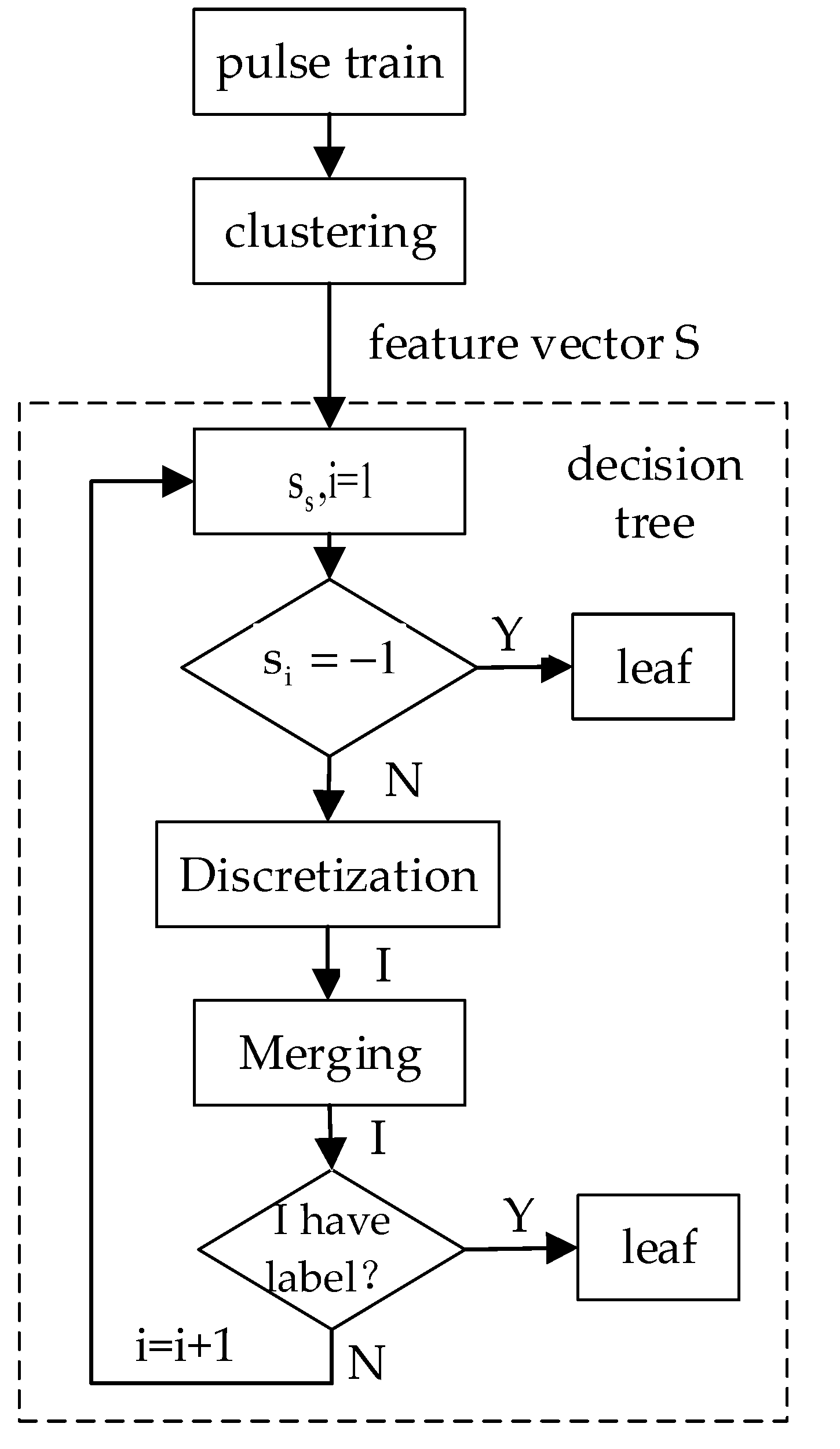
The complete algorithm flow chart is shown in Figure 3. The intercepted radar pulse train is processed by the clustering module to obtain the feature vector. The feature vector set obtained from the training set is input into the decision tree construction module to construct the recognition model. First, at the root node of the tree for each level, at a single time step, we determine whether the eigenvalue of the first dimension of the sample is a marker feature. If so, the sample belongs to a leaf node; then, the remaining samples are discretized into multiple intervals, after which adjacent intervals are fused. If the interval has a class label, after measurement, it is used as a leaf node; if not, it is used as an intermediate node. Then, the next-dimensional feature is selected to continue the analysis recursively until all training samples are assigned to leaf nodes and the decision tree model is constructed.
To identify the intercepted unknown radar signal, we first obtained the repeated frequency eigenvector through clustering, moved through each layer of the constructed decision tree model, compared the eigenvalue in the eigenvector and identified which sub-node belonged to the same level. This was repeated recursively until the leaf node was reached; additionally, the label of the leaf node is the category of the radar signal.
Decision trees can provide a path from the root node to the leaf node for each training sample. Even in the presence of data noise, relying on many training samples can improve the robustness of the algorithm to data noise.

4. Experiment

4.1. Parameter Settings

The experiment mainly focused on the identification of fixed repetition frequency and staggered repetition frequency radars. This section simulates four types of radar pulse data and their parameters are shown in Table 2. Different types of pulse sequence characteristics are indistinguishable from a statistical point of view.
To simulate the measurement error in a real-world measurement environment, a Gaussian distribution-based measurement error (STD) was added to the pulse arrival time. All pulse sequences have different degrees of missing pulses (pulse missing rate) and spurious pulses, and the two kinds of pulses appear randomly with a certain probability. Table 3 shows the specific values of the parameters used for the simulation. The number of training samples of each type is the same for all methods and there is no imbalance in the number of samples. A total of 100 experiments were performed for each scenario.

4.2. Result

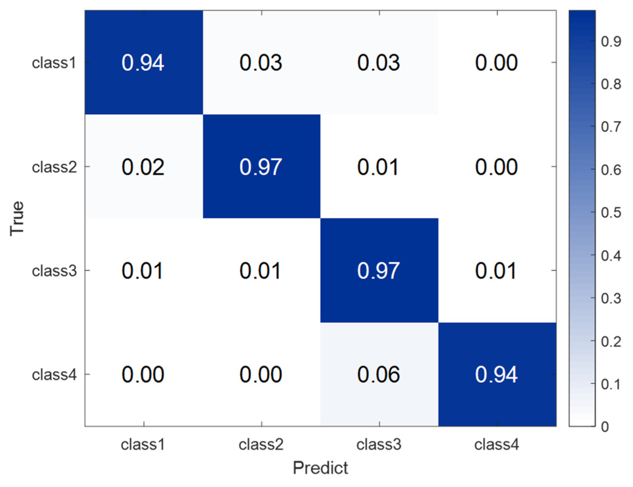
To demonstrate the performance of the proposed method, we tested the recognition accuracy of the proposed method for each type of radar. In the experiment, the leakage pulse rate and interference pulse rate in all pulse trains were 20%, and the number of pulses contained in each pulse train sample was 300. The number of training samples of each type was 500 and the number of test samples was 200. The confusion matrix of the obtained recognition effect is shown in Figure 4. The abscissa represents the predicted category label output by the model; the ordinate represents the real category label. The values on the diagonal of the confusion matrix represent the results of correct classification, while the non-diagonal values represent the result of being classified into other classes. Figure 4 shows that for certain data noise, the recognition accuracy of this method for each category can reach approximately 95%, and our method displays good recognition performance.

5. Discussion

In practical applications, choosing the appropriate size of a training sample set and the length of each pulse train sample is a vital task. A large raining sample will result in an unnecessary waste of computing resources. The data noise in the pulse train will also affect the recognition performance. Therefore, in this section, we study the impact of these factors on recognition performance.
The proposed method is compared with a long-term and short-term memory network (LSTM) [33] (the input is the unprocessed radar pulse train) and support vector machine [18] (the input is the mean and variance of the clustered parameters).

5.1. Influence of Missing Pulse Rate on Recognition Accuracy

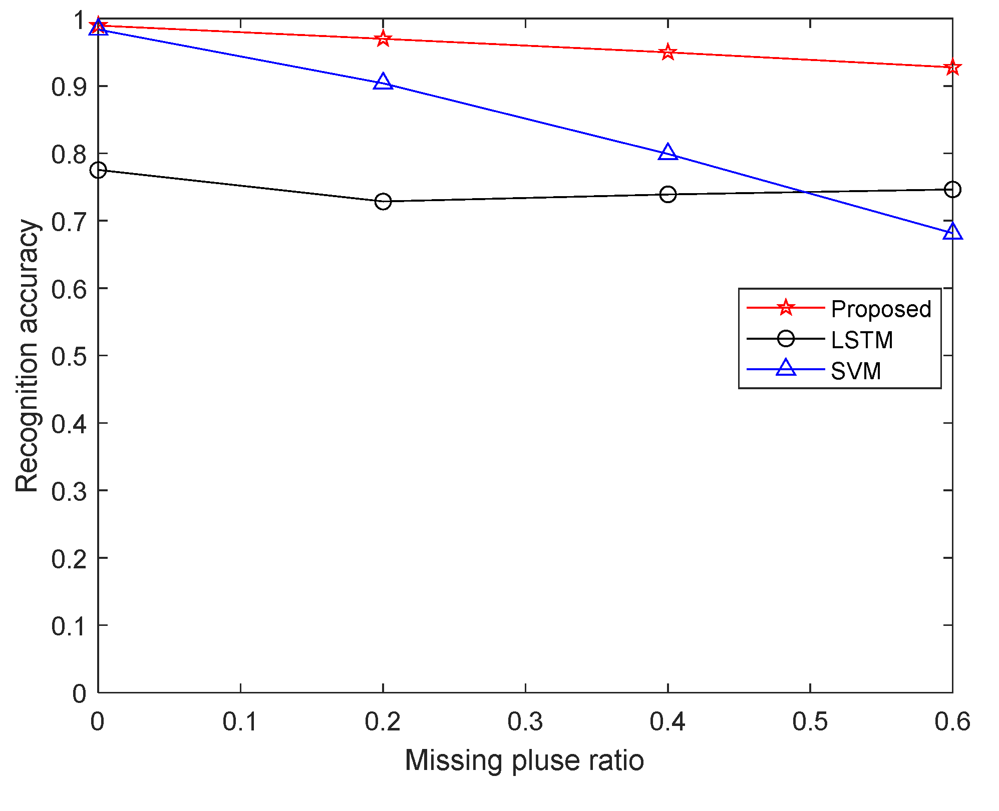
This group of experiments considered the influence of missing pulse rates on the recognition performance. The number of pulses in each pulse train is 300, a set of pulses are lost randomly and the rate of missing pulses increases from 0 to 60% at 20% intervals. In this test, there was no interference pulse, the number of training samples for each type was 500, and the number of test samples was 200. The average recognition rates under different conditions are shown in Figure 5.
Figure 5 shows that the average recognition accuracy of the three methods decreases with the increase in the missing pulse rate; however, our method has great advantages over the other two LSTM methods. Even if the pulse missing rate reaches 60%, the accuracy of the proposed method can reach more than 90%. The simulation results show that this method is suitable to the recognition of radar signals with a high missing pulse rate.

5.2. Influence of Spurious Pulse Rate on Recognition Accuracy

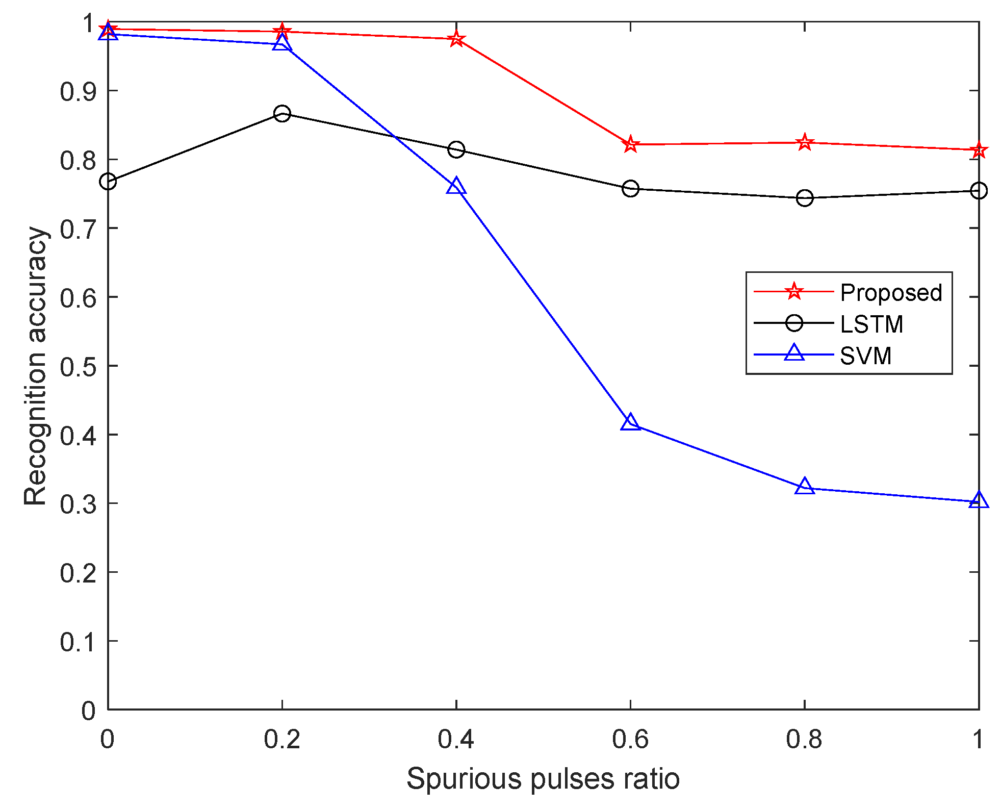
This group of experiments considered the influence of different spurious pulse rates on recognition performance. No pulses are lost, and the spurious pulse rate increased from 0 to 1 in 20% increments. The remaining conditions are the same as in the previous group. The average recognition rates under these different conditions are shown in Figure 6.
Figure 6 shows that with an increase in the spurious pulse rate, the average recognition accuracy of the three methods decreases, but the recognition rate of our method is higher than that of the other two methods. When the spurious pulse rate was higher than 50%, the recognition accuracy of our method suddenly decreases, because the spurious pulse severely damaged the structure of the pulse train. Therefore, if there are too many spurious pulses in the pulse train, the large amount of data noise (in the features) extracted by the clustering module greatly reduces the availability of the extracted accurate features, resulting in a reduction in the recognition rate.

5.3. Influence of Number of Pulses in Pulse Train on Recognition Accuracy

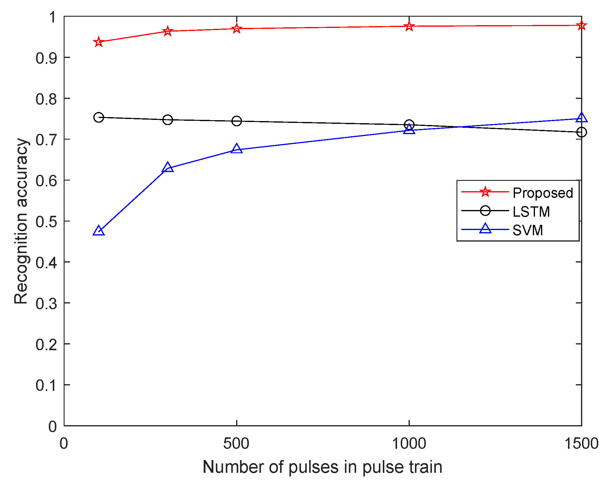
This group of experiments considered the effect of pulse train length on recognition performance. Pulses in the pulse train are lost randomly, and the rate of missing pulses and spurious pulses are both approximately 20%. Several groups of experiments were simulated, and each pulse train in each group contained a different number of pulses, including 100, 300, 500, 1000, and 1500. The remaining conditions were the same as in the previous group. The average recognition rates under different conditions are shown in Figure 7.
When adding data noise, the recognition performance of LSTM and SVM is greatly affected. Even if the number of pulses in the pulse train increases, the recognition rate of both is less than 80%. However, our method has a strong anti-noise ability. When the number of pulses in the pulse train decreases, e.g., to 100, the recognition accuracy of this method reaches approximately 92%. When the number of pulses is 300, the maximum recognition accuracy can be achieved and maintained, so it is appropriate to intercept more than 300 pulses in practical applications.

5.4. Influence of Training Samples Number on Recognition Accuracy

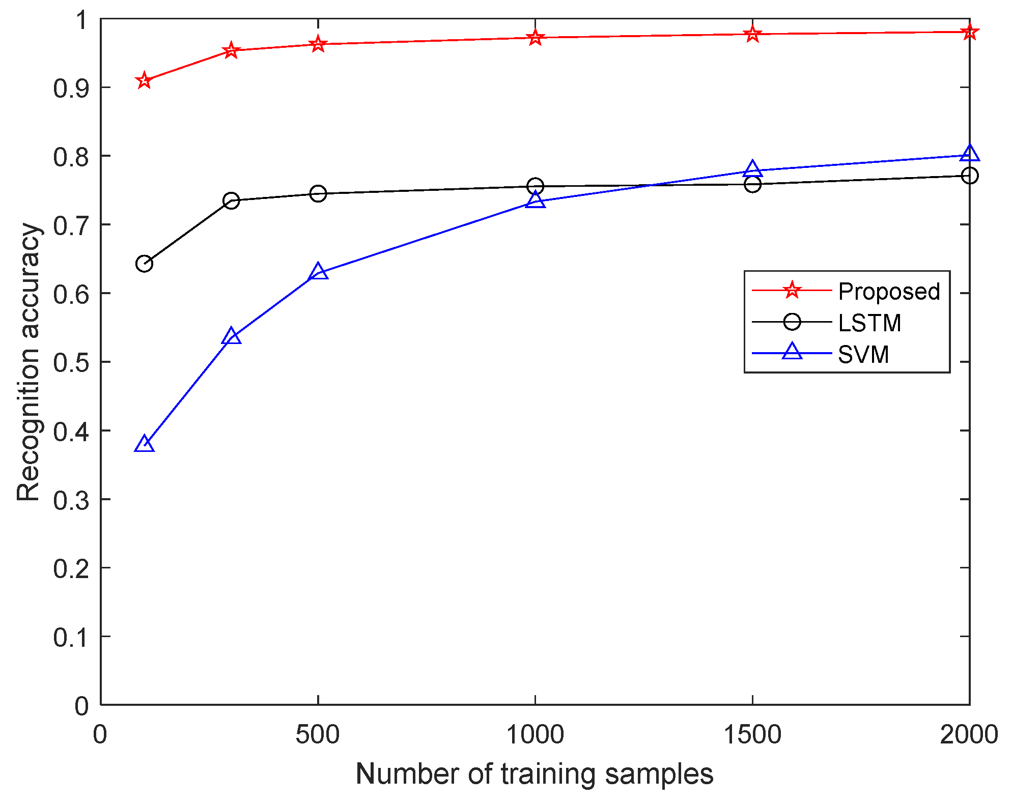
This group of experiments considered the effect of pulse train length on recognition performance. Each pulse is lost randomly, and the rate of missing pulses and spurious pulses are both 20%. There are 100, 300, 500, 1000, 1500, and 2000 scenarios for each type of training sample, and the number of test samples is 200. The average recognition rate under various conditions is shown in Figure 8.
Figure 8 shows that the number of training samples has little impact on our method. Even if the number of training samples is only 100, the recognition accuracy of this method can reach over 90%, while the recognition accuracy of the LSTM neural network method reaches a recognition accuracy of less than 70% with small samples. SVM is more affected by the number of training samples.

6. Conclusions

In this paper, we developed a new methodology for Radar Emitter Recognition (RER) based on parameter set clustering and classification. Unlike other traditional methods, our method directly extracts the typical value of the parameter rather than the statistical features such as the mean and variance of the parameter as the input of the classifier, which effectively reduces the impact of data noise. The simulation results show that our method has good effects. We demonstrated the effect of practical factors on the recognition effect, including missing pulses, spurious pulses, etc. It was found that even if the missing pulse rate is 60%, the recognition accuracy is more than 90%. The recognition accuracy of our method is 96% when the spurious pulse rate is less than 40%, and even if the spurious pulse rate is 1, the recognition accuracy of our method can be 80%. We also demonstrated the effect of a variety of data volumes. When the number of pulses in the intercepted pulse column is more than 300, our method can achieve the maximum recognition performance. When the number of training samples of each type is 100, the method formulated in this work reaches a recognition accuracy of 90%, which means this algorithm can effectively manage recognition problems with small training samples.
In future work, we will focus on the open set recognition problem, forming a new model on the basis of the model that has been produced, rather than retraining all the datasets.

Author Contributions

Conceptualization, T.X., S.Y. and Z.L.; methodology, T.X.; software, T.X.; validation, T.X., Z.L. and F.G.; formal analysis, T.X.; investigation, T.X.; resources, F.G.; data curation, T.X.; writing—original draft preparation, T.X.; writing—review and editing, Z.L. and F.G.; visualization, T.X.; supervision, Z.L. and F.G.; project administration, Z.L. All authors have read and agreed to the published version of the manuscript.

Funding

Outstanding Youth Project of Hunan Province (No. 2020JJ2037).

Data Availability Statement

Not applicable.

Acknowledgments

The authors would like to express their gratitude to the editors and the reviewers for their insightful comments.

Conflicts of Interest

The authors declare no conflict of interest.

Abbreviations

The following abbreviations were used in this manuscript:
AOAAngle of Arrival
CNNConvolutional Neural Network
ESMElectronic Support Measures
LSTMLong Short-term Memory
PAPulse Amplitude
PDWPulse Descriptor Word
PRIPulse Repetition Interval
PWPulse Width
RERRadar Emitter Recognition
RNNRecurrent Neural Network
SVMSupport Vector Machine
TDOATime Difference of Arrival
TOATime of Arrival

References

  1. Liu, J.; Lee, J.; Li, L.; Luo, Z.-Q.; Wong, K. Online clustering algorithms for radar emitter classification. IEEE Trans. Pattern Anal. Mach. Intell. 2005, 27, 1185–1196. [Google Scholar] [PubMed]
  2. Spezio, A.E. Electronic warfare systems. IEEE Trans. Microw. Theory Techn. 2002, 50, 633–644. [Google Scholar] [CrossRef]
  3. Zhou, Y.Y.; An, W.; Guo, F.C.; Liu, Z.; Jiang, W. Principles and Technologies of Electronic Warfare System; Publishing House of Electronics Industry: Beijing, China, 2014; pp. 101–103. [Google Scholar]
  4. Wiley, R.G. ELINT: The Interception Analysis Radar Signals; Artech House: Norwood, MA, USA, 2006. [Google Scholar]
  5. Wu, B.; Yuan, S.; Li, P.; Jing, Z.; Huang, S.; Zhao, Y. Radar Emitter Signal Recognition Based on One-Dimensional Convolutional Neural Network with Attention Mechanism. Sensors 2020, 20, 6350. [Google Scholar] [CrossRef]
  6. Revillon, G. Radar emitters classification and clustering with a scale mixture of normal distributions. IET Radar Sonar Navig. 2019, 13, 128–138. [Google Scholar]
  7. Willson, G.B. Radar Classification Using a Neural Network. Appl. Artif. Neural Netw. 1990, 1294, 200–210. [Google Scholar]
  8. Zhang, W.J.; Fan, F.H.; Tan, Y. Application of cluster method to radar signal sorting. Radar Sci. Technol. 2004, 2, 219–223. [Google Scholar]
  9. Ye, F.; Luo, J.Q. A multi-parameter synthetic signal sorting algorithm based on BFSN clustering. Radar ECM 2005, 2, 43–45. [Google Scholar]
  10. Wang, S.-Q.; Zhang, D.-F.; Bi, D.-Y.; Yong, X.-J. Multi-parameter radar signal sorting method based on fast support vector clustering and similitude entropy. J. Electron. Inf. Technol. 2011, 33, 2735–2741. [Google Scholar] [CrossRef]
  11. Li, Y.; Zhang, M.; Chen, C. A Deep-Learning Intelligent System Incorporating Data Augmentation for Short-Term Voltage Stability Assessment of Power Systems. Appl. Energy 2022, 308, 118347. [Google Scholar] [CrossRef]
  12. Lee, S.K.; Han, B.B.; Rhee, M.K.; Churl, H.J. Classification of the trained and untrained emitter types based on class probability output networks. Neurocomputing 2017, 248, 67–75. [Google Scholar]
  13. Feng, Y.; Cheng, Y.; Wang, G.; Xu, X.; Han, H.; Wu, R. Radar Emitter Identification under Transfer Learning and Online Learning. Information 2020, 11, 15. [Google Scholar] [CrossRef]
  14. Feng, Y.; Wang, G.; Liu, Z.; Feng, R.; Chen, X.; Tai, N. An Unknown Radar Emitter Identification Method Based on Semi-Supervised and Transfer Learning. Algorithms 2019, 12, 271. [Google Scholar] [CrossRef]
  15. Meng, X.P.; Shang, C.X.; Dong, J.; Fu, X.J.; Lang, P. Automatic modulation classification of noise-like radar intrapulse signals using cascade classifier. ETRI J. 2021, 43, 991–1003. [Google Scholar]
  16. Xue, J.; Tang, L.; Zhang, X.G.; Jin, L. A Novel Method of Radar Emitter Identification Based on the Coherent Feature. Appl. Sci. 2020, 10, 5256. [Google Scholar] [CrossRef]
  17. Zhang, Z.; Li, Y.B.; Jin, S.S.; Zhang, Z.Y.; Wang, H.; Qi, L.; Zhou, R.L. Modulation Signal Recognition Based on Information Entropy and Ensemble Learning. Entropy 2018, 20, 198. [Google Scholar]
  18. Zhang, G.X.; Jin, W.D.; Hu, L.Z. Radar emitter signal recognition based on support vector machines. In Proceedings of the ICARCV 2004 8th Control, Automation, Robotics and Vision Conference, Kunming, China, 6–9 December 2004. [Google Scholar]
  19. Liu, Z.M. Multi-feature fusion for specific emitter identification via deep ensemble learning. Digit. Signal Processing 2020, 110, 102939. [Google Scholar] [CrossRef]
  20. Jordanov, I.N.; Petrov, N.; Roe, J. Radar Emitter Signals Recognition and Classification with Feedforward Networks. Procedia Comput. Sci. 2013, 22, 1192–1200. [Google Scholar]
  21. Shieh, C.; Lin, C. A vector neural network for emitter identification. IEEE Trans. Antennas Propag. 2002, 50, 1120–1127. [Google Scholar] [CrossRef] [Green Version]
  22. Zhang, Z.C.; Guan, X.; He, Y. Study on radar emitter recognition signal based on rough sets and RBF neural network. In Proceedings of the 2009 International Conference on Machine Learning and Cybernetics, Baoding, China, 12–15 July 2009. [Google Scholar]
  23. Yin, Z.; Yang, W.; Yang, Z.; Zuo, L.; Gao, H. A study on radar emitter recognition based on SPDS neural network. Inf. Technol. J. 2011, 10, 883–888. [Google Scholar] [CrossRef]
  24. Liu, Z.M.; Yu, P.S. Classification, Denoising, and Deinterleaving of Pulse Streams with Recurrent Neural Networks. IEEE Trans. Aerosp. Electron. Systems 2019, 55, 1624–1639. [Google Scholar] [CrossRef]
  25. Li, X.Q.; Liu, Z.M.; Huang, Z.T.; Liu, W.S. Radar Emitter Classification with Attention-Based Multi-RNNs. IEEE Commun. Lett. 2020, 24, 2000–2004. [Google Scholar] [CrossRef]
  26. Liao, X.; Li, B.; Yang, B. A Novel Classification and Identification Scheme of Emitter Signals Based on Ward’s Clustering and Probabilistic Neural Networks with Correlation Analysis. Comput. Intell. Neurosci. 2018, 2018, 1458962. [Google Scholar] [CrossRef] [PubMed]
  27. Guo, S.; White, R.E.; Low, M. A comparison study of radar emitter identification based on signal transients. In Proceedings of the 2018 IEEE Radar Conference, Oklahoma City, OK, USA, 23–27 April 2018. [Google Scholar]
  28. Ford, B.P.; Middlebrook, V.S. Using a knowledge-based system for emitter classification and ambiguity resolution. In Proceedings of the IEEE National Aerospace and Electronics Conference, Dayton, OH, USA, 22–26 May 1989. [Google Scholar]
  29. Anderson, J.A.; Gately, M.T.; Penz, P.A.; Collins, D.R. Radar Signal Categorization Using A Neural Network. Proc. IEEE 1990, 78, 1646–1657. [Google Scholar] [CrossRef]
  30. Cheng, Y. Mean Shift, Mode Seeking, and Clustering. IEEE Trans. Pattern Anal. Mach. Intell. 1995, 17, 790–799. [Google Scholar] [CrossRef]
  31. Kuang, W.; Chan, Y.; Tsang, S.; Siu, W. Machine Learning-Based Fast Intra Mode Decision for HEVC Screen Content Coding via Decision Trees. IEEE Trans. Circuits Syst. Video 2020, 30, 1481–1496. [Google Scholar] [CrossRef]
  32. Müller, W.; Wysotzki, F. Automatic construction of decision trees for classification. Ann. Oper. Res. 1994, 52, 231–247. [Google Scholar] [CrossRef]
  33. Chikkamath, S.; SR Nirmala, S.R. Melody generation using LSTM and BI-LSTM Network. In Proceedings of the 2021 International Conference on Computational Intelligence and Computing Applications, Nagpur, India, 26–27 November 2021. [Google Scholar]
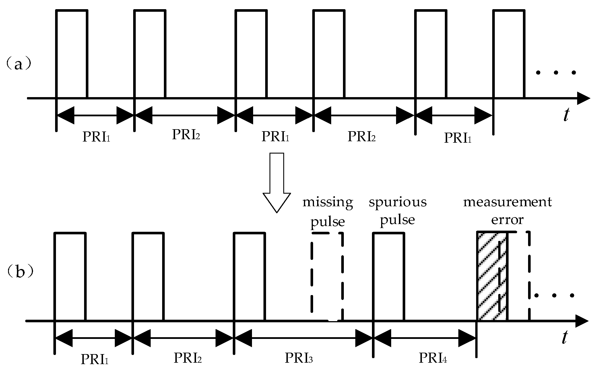
Figure 1. Data noise in pulse train. (a) Pulse train without data noise. (b) Pulse train with data noise.
Remotesensing 14 04468 g001
Figure 2. Decision tree.
Remotesensing 14 04468 g002
Figure 3. Process of recognition.
Remotesensing 14 04468 g003
Figure 4. Confusion matrix of recognition effect.
Remotesensing 14 04468 g004
Figure 5. Average recognition accuracy under different leakage pulse rates.
Remotesensing 14 04468 g005
Figure 6. Average recognition accuracy under different interference pulse rates.
Remotesensing 14 04468 g006
Figure 7. Average recognition accuracy under different pulse train lengths.
Remotesensing 14 04468 g007
Figure 8. Average recognition accuracy under different numbers of training samples.
Remotesensing 14 04468 g008
Table 1. Samples.
Table 1. Samples.
SampleFeature VectorLabel
1 [100,−1]a
2 [100,300,−1]b
3 [300,100,−1]b
4 [300,100,200,−1]c
5 [200,100,300,−1]c
6 [100,300,200,400,−1]d
7 [200,400,100,300,−1]d
Table 2. Simulation parameters.
Radar TypePRI TypePRI Model (us)STD (μs)
1fixed3002
2staggered [100 300 500]2
3staggered [100 300 500 700]2
4staggered [100 320 500 700]2
Table 3. Parameter setting.
ModuleParameterValue
clusteringPRI upper bound PRImax2000 µs
PRI lower bound PRImin50 µs
Radius h 0.03
frequency threshold factor λ 0.08
decision treeThreshold S 0.95
Confidence α 0.997
Publisher’s Note: MDPI stays neutral with regard to jurisdictional claims in published maps and institutional affiliations.