Abstract
The fall armyworm (FAW) (Spodoptera frugiperda) (J. E. Smith) is a migratory pest that lacks diapause and has raised widespread concern in recent years due to its global dispersal and infestation. Seasonal environmental changes lead to its large-scale seasonal activities, and quantitative simulations of its dispersal patterns and spatiotemporal distribution facilitate integrated pest management. Based on remote sensing data and meteorological assimilation products, we constructed a mechanistic model of the dynamic distribution of FAW (FAW-DDM) by integrating weather-driven flight of FAW with host plant phenology and environmental suitability. The potential distribution of FAW in China from February to August 2020 was simulated. The results showed a significant linear relationship between the dates of the first simulated invasion and the first observed invasion of FAW in 125 cities (R2 = 0.623; p < 0.001). From February to April, FAW was distributed in the Southwestern and Southern Mountain maize regions mainly due to environmental influences. From May to June, FAW spread rapidly, and reached the Huanghuaihai and North China maize regions between June to August. Our results can help in developing pest prevention and control strategies with data on specific times and locations, reducing the impact of FAW on food security.
1. Introduction
Seasonal changes in the global environment can lead to large-scale seasonal movements of migratory insects and dynamic changes in their spatial distribution and abundance [1,2]. Shifting seasonal activities is an important survival strategy for migratory pests [3]. When regional environments are unsuitable or food resources are unavailable, pests will invade and develop new breeding areas, causing substantial ecological and economic damage [4,5]. The fall armyworm (FAW), Spodoptera frugiperda (J. E. Smith) is a migratory pest that has affected more than 70 countries worldwide in recent years [6]. FAW lacks diapause [7] and its winter breeding area is limited to tropical and subtropical regions, but it has a strong migratory ability, and its seasonal invasion is widespread [8]. Based on insect radar and sex hormone trap records, FAW has been found to survive in winter breeding areas below 28°N in the United States. As temperatures gradually rise and crops are planted, FAW has the potential to spread northwards to Canada [9,10]. Prediction of pest population dynamics is critical for assessing the risk of pest outbreaks, and understanding their spatio-temporal distribution facilitates integrated pest management (IPM) [11,12].
The FAW invaded China at the end of 2018, and spread widely in 2019 [13]. Due to the lack of experience in controlling FAW in China, FAW damaged 1.125 and 1.278 million hectares of crops in 2019 and 2020, respectively [14]. The latitudinal range of the main maize production area in eastern China is similar to that of the United States, which is one of the native habitats of the FAW [15]. Some seasonal FAW activities have been observed in China [16,17,18], but a quantitative dynamic distribution model is still needed to further reveal the migration pattern and spatial distribution of the FAW.
Correlative species distribution models (SDMs) and numerical trajectory models are commonly used to predict the spatial distribution of FAW. Correlative SDMs (including statistical models and machine learning models) calculate the distribution probability and severity of FAW outbreaks based on climate suitability deduced from FAW presence/absence data [19,20,21]. Whereas, numerical trajectory models such as the Hybrid Single-Particle Lagrangian Integrated Trajectory model (HYSPLIT) from the National Oceanic and Atmospheric Administration (NOAA) and the Numerical Atmospheric-Dispersion Modelling Environment model (NAME) from the UK Met Office, rely on atmospheric conditions, including pressure, wind speed, and wind direction to analyze the potential migration routes and landing areas of FAW [22,23]. Overall, the correlative SDMs and the numerical trajectory models have advantages in spatial and temporal continuity, respectively, and can effectively simulate insect distribution. However, correlative SDMs are commonly employed to exploit “static“ ecological niches of pests due to dispersal limitations and climate-location bias [24]. The accuracy of numerical trajectory models is also restricted by their reliance on atmospheric conditions and lack of consideration of the effects of environmental conditions on pest life cycles [25]. Current models have trouble clarifying the mechanistic relationships between insect dispersal, host plants, and the environment. The causes of pest outbreaks are complex, and outbreak risks are determined by the synergy of pest physiology and the external environment [26]. Thus, this study aims to couple the numerical trajectory models with the mechanistic SDMs that consider the physiological reflection of FAW to the environment, i.e., the eco-physiological model [27], so that the prediction results can reflect the dispersal process of the FAW, as well as changes in population dynamics.
In dynamic species ecological niche studies, remote sensing and meteorological assimilation products are increasingly employed for their high spatial and temporal resolution [28]. On the one hand, insects are sensitive to meteorological fluctuations due to their ectothermic physiology [12], therefore spatiotemporal continuous meteorological assimilation data, such as temperature, precipitation, and humidity, are needed as the basis for mechanistic models of insect growth, survival, and fecundity [29,30]. On the other hand, the use of remote sensing to finely characterize insect habitats helps to quantify the environmental conditions experienced by insects and capture their spatial distribution and population dynamics [31]. Particularly for host plants, using the remote sensing phenology model as an alternative to the traditional degree-days model can obtain more precise data on their spatial and temporal availability and phenological stages on a large scale and at low cost [32,33,34], which can be used as indicators to study the restricted extent and time of pest invasion risk to target regions.
Overall, pest distribution modeling is developing toward integrating multi-factors, dynamic and explicit processes. Based on continuous observation of complex geographic scenarios from remote sensing and meteorological assimilation products, we developed a FAW dynamic distribution model (FAW-DDM). This is supported by a theoretical framework related to the life cycle of the FAW, encompassing the effects of migration, host plants, and the environment on the distribution of the FAW. We applied the FAW-DDM model to simulate the dynamic distribution of FAW in China from February to August 2020. The results can play an important role in providing information to support the formulation of precise control strategies.
2. Materials and Methods
2.1. Study Area and Multisource Data
2.1.1. Study Area and Distribution Data of FAW
China is influenced by the East Asian monsoon, with southwesterly winds prevailing in spring and summer, and northerly winds in autumn and winter [15]. The local FAW in the annual breeding area and the invasive FAW from Southeast Asia can disperse northward under suitable conditions with the help of favorable seasonal wind currents. The main strains of FAW that invaded China were maize strains, and the damage caused by the FAW to maize far exceeds that of other crops in China [14,35]. Also, western China, especially the Qinghai-Tibet Plateau, has the advantage of a natural barrier to insect invasion--its high altitude. Thus, we focused on four major maize growing regions in eastern China (Figure 1), which account for more than 90% of the total annual production of maize in China [36].
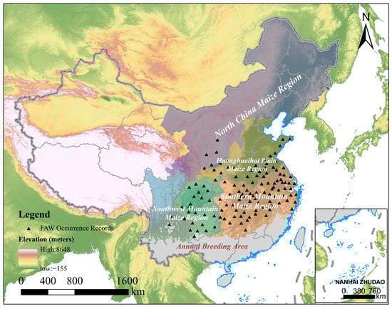
Figure 1.
The geographical location of the study area and FAW occurrence records. The gray area represents the annual breeding area, i.e. the area where the average temperature of the coldest month (January) is greater than 10 °C and FAW and host plants can grow here year-round [22]; the Digital Elevation Model (DEM) available from USGS [37]; and the shapefile of four major maize growing regions in China available from http://region.agridata.cn/ (accessed on 16 February 2022).
We collected the dates and geographic locations of the FAW captures recorded in the literature, news reports, and county and municipal level plant protection station surveys in 125 cities. We conducted overlay analysis to filter out FAW occurrence records in annual breeding areas, and performed Zonal Statistics to keep the earliest invasion records within one city, as shown in Table S1, to verify the accuracy and performance of the FAW-DDM.
2.1.2. Atmospheric Conditions
Final Analysis (FNL) data, a six-hourly, 1° 1° grid, global meteorological dataset from the National Centers for Environmental Prediction (NCEP) [38], were used as the initial and boundary conditions for the Weather Research and Forecasting (WRF) model (version 3.8, www.wrf-model.org, accessed on 16 February 2022) [39], to produce the atmospheric conditions for the trajectory calculations. WRF model forecast time is 72 h and outputs data for horizontal and vertical windspeed, pressure, and precipitation at 1-h intervals [40]. The parameters of the WRF model were set as shown in Table 1.

Table 1.
Parameters for the Weather Research and Forecasting (WRF) model.
2.1.3. Vegetation Data
The Global Land Surface Satellite (GLASS) Leaf Area Index (LAI) product [41] was used to extract the phenology of the main host plant maize. The GLASS LAI product was developed by inputting the fused LAI MODIS product, CYCLOPES LAI products, and the reprocessed MODIS reflectance of the BELMANIP sites during the period 2001–2003, into the general regression neural networks (GRNNs) for training [42]. GLASS LAI product has a spatial resolution of 1 km and a temporal resolution of 8 days. The 2010 and 2015 cropland layers from the 1 km National Land Cover Dataset (NLCD) of China [43] were used as a mask to determine the planting range of the crops (http://www.resdc.cn/Default.aspx, accessed on 16 February 2022).
2.1.4. Environmental Data
The environmental data is from the European Centre for Medium Range Weather Forecasts (ECMWF) and is hourly product from the enhanced fifth generation of European ReAnalysis (ERA5-Land) [44]. The ERA5-Land data product has a spatial resolution of 0.1 radians 0.1 radians (~10 km). We used Google Earth Engine (https://earthengine.google.com/, accessed on 16 February 2022) to batch acquire and process the daily average data of the 2-m air temperature “temperature_2m” and the water content in the soil layer (0–7 cm) “volumetric_soil_water_layer_1” [45] in 2020, to assess the environmental effects on growth and development of the FAW.
2.2. Modeling the Dynamic Spatial Distribution of FAW
The dynamic distribution model for the FAW (FAW-DDM) was developed by considering the eco-physiological characteristics of the FAW and the external environmental conditions. The FAW-DDM includes three modules, namely insect migration simulation, host plant phenology extraction, and environmental suitability analysis. The three modules are linked and iteratively invoked through the life cycles of the FAW. The methodological framework of this study is shown in Figure 2 and is described as follows: (1) The insect migration simulation module is used to predict the weather-driven flight of FAW, and finds its possible invasion area. (2) The host plant phenology extraction module allows us to examine whether the maize in the potential invasion area has been planted or harvested, i.e., whether it can provide food resources for the growth and development of the FAW. (3) The environmental suitability analysis module can be used to evaluate whether the environment is suitable for the FAW, and to calculate the growth rate of the FAW under current environmental conditions. Thus, the timespan for the next generation of FAW to develop from eggs to adults and the time of the next migration can be estimated. (4) By iterating the above steps, the spatial distribution and population dynamics of FAW can be determined for each period.
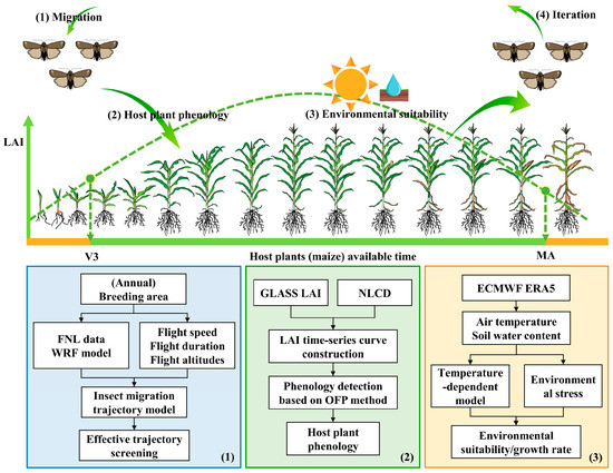
Figure 2.
Methodological framework. Steps 1–4 in the upper part show a schematic representation of the FAW life cycle (described in the text). These steps are linked to the three modules presented in boxes in the lower part, which show the corresponding technical flow: (Box 1) Insect migration simulation module; (Box 2) Host plant phenology extraction module; (Box 3) Environmental suitability analysis module. A portion of the image materials is sourced from [46,47].
2.2.1. Simulation of Numerical Migratory Trajectories of FAW
The atmospheric conditions simulated by WRF were used as input data for the 3D insect numerical trajectory analysis program developed by [48], based on the FORTRAN language, to calculate the possible atmospheric dispersion paths of the FAW [17]. The forward trajectories in February of the FAW began in the annual breeding area of China as well as Southeast Asia [22,35]. The nightly starting points of migration were evenly distributed within a 1° 1° grid, including parts of Yunnan, Hainan, Guangxi, Guangdong, and Fujian provinces, and the Indochina Peninsula including Laos, Vietnam, and Myanmar, where FAW had been detected [49], as shown in Figure S1. The starting points of the forward trajectories from March to August were determined using the spatial distribution of FAW calculated during the previous month.
Based on the biological characteristics of the FAW, the migration parameters used in the trajectory simulations in this study were set as follows: (1) Flight duration: FAW can fly continuously for 10 h per night. Depending on the geographical location of the current simulation area and sunlight condition, FAW was set to take off at dusk (19:00) and stop flying at dawn (05:00) the next day [17,49]. FAW can fly continuously for three nights under suitable environmental conditions [22,50]. If the FAW enter a large area of water, the single flight time was extended to a maximum of 36 h [40]. (2) Flight speed: The self-powered flight speed of noctuid moths with a similar body size to the FAW was 2.5–4 m/s. The self-powered flight speeds of FAW were set as 3 m/s [15]. (3) Flight altitude: Noctuid moths usually migrate at altitudes with low level jet streams (wind speeds greater than 10 m/s) [51]. To ensure that the most probable flight altitude could be found, the altitudes of 500, 750, 1000, 1250, 1500, 1750, 2000, and 2250 m above sea level [15] were used in combination with the Digital Elevation Model (DEM) [37] to calculate the trajectory. (4) Forced landing factors: The migration insects will stop flying when the air temperature is below their low temperature threshold for flight. When the temperature at the flight altitude of the FAW is below its low temperature threshold for the flight of 13.8 °C [15,40,52,53], the trajectory calculation will be terminated for that night. When the hourly rainfall is greater than 1 mm (moderate rain and above), the FAW will be affected by the rainfall and be forced to land [17]. If there is rain or other factors affecting take-off at dusk, we assume that FAW will not take off again that night, and the FAW will develop in this area [54]. The trajectories that meet these requirements and their starting and landing points that were not in a large area of water were selected as effective trajectories to determine the location of potential invasion areas for the FAW.
2.2.2. Extraction of the Phenology of the Main Host Plant Maize
The optimal filter-based phenology detection method (OFP) [55] was used to extract the phenology of maize, which is the main host plant of FAW. (1) LAI time series curve construction: The GLASS LAI product was used to create annual time series curves of the LAI for the cropland grid of the NLCD mask. The dual logic (DL) method, Savitzky-Golay (SG) filter method, and the wavelet-based filter (WF) method were used to smooth the LAI time series curves, respectively. (2) Extraction of key phenological stages: The key maize phenological stages were identified using the inflection points and the thresholds of the smoothed LAI time series curves, where the first derivative was increasing, and the second derivative was equal to zero was defined as the maize 3rd leaf stage (V3). The date when the LAI reached its maximum value was defined as the heading stage (HE), and the inflection point where the first derivative was negative and had the largest absolute value was defined as the maturity stage (MA) [56,57]. (3) Optimal LAI smoothing method selection: The RMSE values for the estimated and observed phenology dates were compared, and the smoothing method with the minimum average RMSE was selected in the provincial range. (4) Application of OFP method: Using the OFP method to detect the dates of key phenological stages in the crop grids in each province, the limited timespans for the three phenological stages of spring and summer maize were determined based on observations from agricultural meteorological stations (AMS). All three phenological stages were required to satisfy the restricted timespan, otherwise, they were not considered to be maize pixels.
According to [55], the related R2 between the estimated maize phenology using the OFP method and the phenology observed by ASM was 0.97 (average RMSE = 6.7; p < 0.01), which had a high level of accuracy. The ChinaCropPhen1km dataset is available at https://doi.org/10.6084/m9.figshare.8313530 (accessed on 25 October 2021). We calculated the mean DOY (day of the year) for maize V3 and MA from 2010 to 2019 using raster statistics on a pixel-by-pixel basis (Figure 3). They were then rescaled to match the simulation of migration trajectories, and the neighborhood mean interpolation method was used to compensate for missing data. Given that the annual breeding areas of Yunnan, Hainan, and Guangxi in China have a favorable climate, host plant maize can be planted throughout the year, and the phenology of the fields varies substantially. According to the field survey, the FAW can also reproduce throughout the year in this range [35], so the phenological restrictions are not considered in the annual breeding area. In addition, the time of invasion and the time of emigration must be within the time range of V3-MA to ensure that food resources can meet the needs for the growth and development of the FAW.
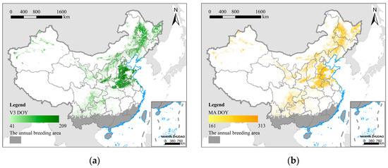
Figure 3.
The mean DOY of the key phenological stages of maize, the main host plant for FAW in China from 2010 to 2019; (a) the 3rd leaf stage (V3); (b) the maturity stage (MA). The dark gray area represents the annual breeding area.
2.2.3. Calculation of Environmental Suitability Using the Eco-physiological Model
The eco-physiological model (also called the mechanistic niche model) was used to calculate the growth rate of the FAW under current environmental conditions, and it can also be used as an indicator of environmental suitability [27]. The population growth model for insects was introduced [58], where represents the intrinsic growth rate of a stable insect population through time . Maino et al. [59] classified into the positive growth rate and the negative growth rate according to the effects of environmental factors on the development of the FAW.
For the calculation of the positive growth rate , the thermal performance curve (TPC) for the FAW was constructed using the Sharpe and DeMichele model [60] in conjunction with the constant and variable temperature experiments of [61]. This reflected the effect of temperature on the development rate and time of the FAW from egg to adult. The descriptions of specific development parameters are shown in Table S2, and the simulation results are shown in Figure S2. The formula is as follows:
For the calculation of the negative growth rate , we considered the effects of cold, heat, and dry stress [62] on the development of the FAW, which were expressed using the 2 m air temperature and the soil water content. When the environment is not suitable for the growth and development of the FAW, it will cause stress death. We can derive by quantifying the average mortality rate per unit of stress and per time caused by environmental variable above a maximum threshold of or below a minimum threshold of . [59] is the survival rate under the cumulative stress in time . The mortality caused by all the stress conditions was cumulatively summed to obtain . The specific eco-physiological parameters are shown in Table 2. If daily is less than zero, it is not included in the cumulative growth rate .
Table 2.
The environmental thresholds and mortality parameters of FAW.
Flying activity accelerates the development of FAW ovaries, and females usually reach their peak egg laying capacity after flight [66]. When the cumulative growth rate is greater than or equal to one from the adult invasion date, it is assumed that the next generation of FAW has developed from egg to adult within that period and has the ability to migrate long distances and can start the next round of migration. The longest cumulative development time for the FAW does not exceed 90 days [67], otherwise, the current environment of this area would be considered unsuitable for the growth and development of the FAW.
3. Results
3.1. Validation of the Results of the Dynamic Spatial Distribution Model of FAW
A total of 898,020 migratory trajectories from February to August 2020 were simulated, and a total of 154,270 trajectories with landing points in areas with available host plants and suitable environments were screened using Python 3.9 (https://www.python.org/, accessed on 16 February 2022). To validate the accuracy and performance of FAW-DDM, this study used the validation method of [22], by comparing the first field observation dates for the FAW in 125 cities with the first FAW invasion dates simulated by the model (Table S1) and a linear regression was established (Figure 4).
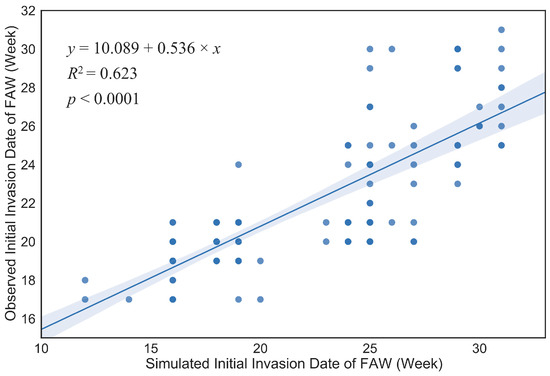
Figure 4.
Linear regression of the observed initial invasion dates (week no.) and simulated initial invasion dates (week no.) of the FAW in 125 municipalities in China; shading is the 95% confidence interval.
In the linear regression model, is the date of the observed initial invasion date of FAW, and is the simulated initial invasion date where the FAW spread to the corresponding area. The two have a significant linear relationship ( = 0.623; = 203.018; = 1,123; < 0.001). Using a paired t-test ( = 0.634, = 124, = 0.527), it was shown that there was no statistically significant difference between the means of the simulated results and the field observations, indicating that the model worked effectively.
3.2. Potential Spatio-Temporal and Relative Abundance of FAW
Kernel density analysis (KDA) was performed on the monthly screened landing points, and the bandwidth was computed using Silverman’s Rule of Thumb and ranked from the smallest to the largest density quantile of the landing points. The results are shown in Figure 5, which indicate the potential spatial distribution range and relative abundance of the FAW from February to August 2020. During this period, FAW populations spread from their overwintering breeding areas in southern and southwestern China to seasonal feeding areas in eastern and northern China.
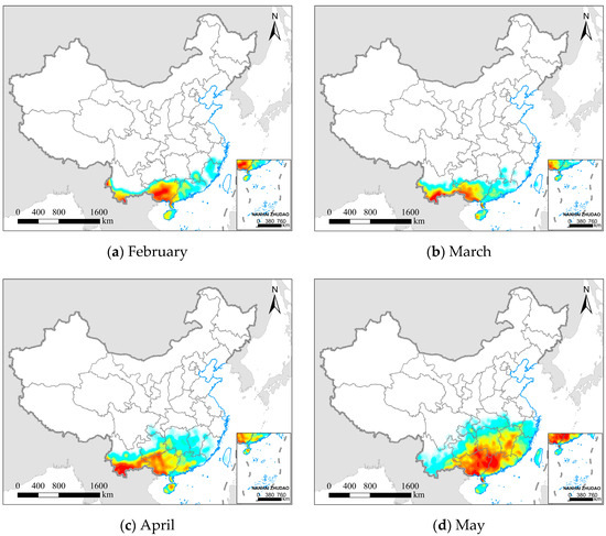
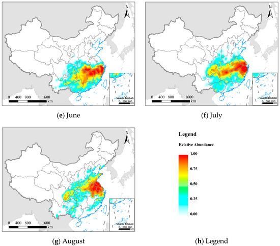
Figure 5.
Spatial distribution and relative abundance of the FAW from February to August 2020. (a–g) represent different months, and (h) the legend from blue to red represents the relative abundance of FAW increasing.
To quantitatively characterize the spatial distribution of the FAW, a combination of box-line and violin plots (RainCloud plots) of the distribution of the FAW for latitude and longitude and their probability density were plotted for each month [68], as shown in Figure 6.
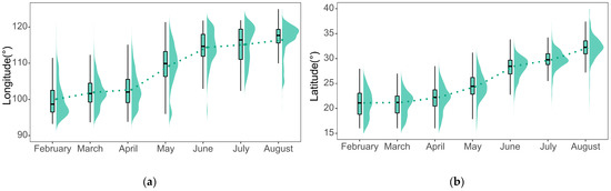
Figure 6.
Spatial distribution and probability density of the FAW at (a) longitude and (b) latitude. The dotted line connecting point is the median of the longitude or latitude of the landing points for each month.
We divided the northward migration process of the FAW in China into three stages based on its spatial distribution characteristics: (1) Overwintering breeding period (February to April): FAW overwintered and reproduced in tropical and subtropical regions of China, and FAW from Southeast Asia also continue to migrate into these regions. From February to March, FAW had relatively little variation in the potential distribution range, and the regions with a higher probability density of FAW (as shown in Table S3) were mainly concentrated in the annual breeding areas of Guangxi (59.63%, 38.34%), Yunnan (19.72%, 46.79%), Guangdong (12.39%, 8.92%), and Hainan (3.90%, 4.30%). In April, with the rising temperature, a small number of FAW adults began to disperse northward into Guizhou (6.16%), Hunan (5.05%), and Jiangxi (1.59%), but the majority of FAW were still distributed in Yunnan (42.44%), Guangxi (30.90%), Guangdong (9.82%), and Hainan (3.37%).
(2) Transitional migration period (May to June): As the environment gradually became favorable for the survival of FAW, the FAW rapidly began to spread north and east from the annual breeding area and its potential distribution range significantly grew. In May, the FAW invasion areas were mainly distributed in the Southwest Mountain maize region and the Southern Mountain maize region, including Guangxi (30.34%), Guangdong (18.42%), Hunan (13.78%), Jiangxi (11.97%), Guizhou (7.03%), Fujian (6.17%), and Yunnan (5.26%). In June, FAW moved out mainly from the southern provinces mentioned above, and the invasion area was predominantly concentrated in the Yangtze River basin, including Jiangxi (21.87%), Hunan (18.52%), Zhejiang (18.43%), Hubei (13.46%), and Guizhou (5.39%). The northern boundary of the potential invasion area has reached the Huanghuaihai Plain maize region, but the FAW populations were relatively few (<1%).
(3) Key preventive period (July to August): The FAW continuously invaded the Huanghuaihai Plain maize region and the North China maize region, which are the main maize planting regions in China and account for more than 60% of the total annual maize production. In July, the FAW were mainly distributed in the middle and lower reaches of the Yangtze River, including Zhejiang (21.22%), Anhui (14.72%), Hunan (13.45%), Hubei (10.64%), Jiangsu (7.84%), and Jiangxi (6.24%). At this time, the FAW was still in the early stages of invading the Huanghuaihai Plain maize region (4.42%), and the northern boundary of the FAW invasion area reached the North China maize region (<1%). In August, the FAW was mainly distributed in the North China Plain, including Anhui (29.77%), Jiangsu (26.56%), Henan (8.60%), and Shandong (7.69%). During this period, FAW populations increased in the Huanghuaihai Plain maize region (34.76%). The North China maize region, including Shaanxi (1.66%), Liaoning (0.60%), Hebei (0.54%), and Shanxi (0.21%) had relatively little FAW.
3.3. Analysis of the Influencing Factors of the Spatial Distribution of FAW
In the model simulation results, the FAW that completed their life cycles in suitable areas accounted for 17.18% of the total simulated amount. To quantitatively evaluate the influencing factors of the FAW in the process of northward migration in China, we calculated the normalized value of the ratio of the trajectories restricted by the following conditions to the total restricted trajectories each month, as the relative impact percentage (RIP) of the factor (Figure 7): (1) Affected by environmental factors (ENV, including air temperature, soil water content), FAW cannot develop and survive normally; (2) FAW migration terminated due to precipitation (PRE); (3) Maize phenology (MAI) did not match the period of the invasion of the FAW, resulting in a lack of food resources.
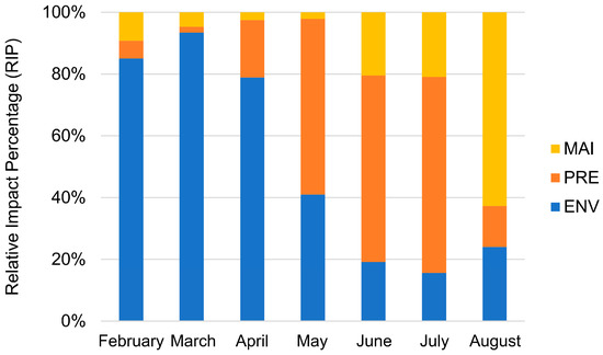
Figure 7.
Relative impact percentage (RIP) of three influencing factors on the distribution of the FAW from February to August 2020.
Before May, environmental factors were the main influencing factor, with an average RIP of 85.8%, from May to July. As the temperature rose (as shown in Figure S3), the environmental suitability increased, and the limitation weakened with an average RIP of 24.92%. In August, environmental limitations began to increase again, with a RIP of 33.25%. The effect of precipitation on FAW trended to increase and then decrease. From May to July with the onset of the rainy season (as shown in Figure S4), the effect of precipitation on FAW increased with an average RIP of 60.32%. Precipitation was the main influencing factor for FAW in this period, and the influence of rainfall weakened after July. The limitation of maize phenology on FAW showed a decreasing and then increasing trend. From February to May, the spread of FAW was limited predominantly due to unsown maize (Invasion DOY < V3 DOY), and this effect was gradually weakened with maize planting. From June to August, the increase in maize maturity and harvesting (Invasion DOY > MA DOY) led to a decrease in available food resources for the FAW. In mid to late August, the growing season was coming to an end in the main maize planting regions, and maize as the host plant became the main influencing factor, with 62.72% of RIP. Overall, the average RIP from February to August showed that environmental factors including air temperature and soil water content had the most pronounced effect on distribution (51.01%), followed by precipitation (31.49%), and maize phenology (17.50%).
4. Discussion
4.1. Strengths and Weaknesses of the Process-Based FAW-DDM Framework
Seasonal activity patterns of insect populations can be used as a basis for predicting large-scale insect outbreaks. Unlike most previous studies that used the correlative SDMs to study the relatively “static” ecological niches of species, in this study, three modules named insect migration simulation, host plant phenology extraction, and environmental suitability analysis were used to link the life cycles of FAW including growth, reproduction, and dispersal, and established a process-explicit modeling framework to iteratively update the “dynamic” spatial distribution of FAW. Meanwhile, we combined the advantages of remote sensing data to observe the environment and host plant phenology, providing spatial and temporal continuous data to simulate the distribution and population dynamics of FAW in China. Our results can reflect the activity of FAW under environmental impact and provide information support for formulating accurate pest control strategies by time and region. In addition, our results can provide a baseline for comparison with the situation after the implementation of control efforts, to evaluate the effectiveness of current pest control measures. With the construction of the digital platform for pesticides and further research into FAW pesticide resistance [69], we can overlay pesticide use condition in the model to obtain more accurate results.
Insects often migrate long distances with the help of favorable seasonal wind currents [51]. The directions, distances, and paths of wind-driven insect migration can be well modeled using atmospheric conditions [22]. In this study, the insect migration simulation module estimated the hourly 3D forward trajectory of FAW using atmospheric conditions generated by WRF for different vertical layers. The numerical trajectory simulation method used in this study has been applied in the migration studies of the FAW by [15,17,40], and the performance of this method has been verified.
As poikilotherms, the life cycle of FAW can be simulated based on the temperature- dependent insect phenology model [64,70,71]. This study employed the Sharpe and DeMichele model in the environmental suitability analysis module, to more accurately describe the nonlinear relationship between insect developmental rate and temperature, thus avoiding the bias of linear phenology models such as the degree-day model at extreme temperatures [72,73]. In addition, the pupation, pupal survival, and emergence of FAW are sensitive to soil moisture, and most mature FAW larvae cannot pupate and survive in dry soil [74], therefore we introduced drought stress to describe the negative effect of moisture on FAW. The FAW is likely to develop local adaptations to the environment after migration to a new region, resulting in greater tolerance to the environment, and allowing it to develop in areas once considered unsuitable for survival. This biological mechanism may also lead to lagging model predictions.
Host plant availability and phenology are also critical in influencing the growth and reproductive processes of pests [11,75]. Host plants are only available as food resources for a limited time during the growing season, and many insect life cycles are closely synchronized with plant phenology [76]. The time-series satellite imageries with wide spatial coverage and short revisit times are widely used for crop phenology extraction studies on the large scale [32,34]. However, the accuracy of crop phenology extraction in the south of China is inevitably lower than that in the north due to the complex planting structure, irregular planting time, as well as cloudy and rainy weather [77], and further model improvement is needed by combining multi-source and multi-scale data and vegetation growth models [78].
Species distribution change is a complex ecological process driven by population dynamics and dispersal, including multiple environment–species interactions [79]. This study employed quantitative and simplified eco-physiological parameters and mathematical models to describe the life history strategies of FAW, and the performance of the models depended largely on the availability of data and prior knowledge. The modular framework also helps to understand the factors influencing the distribution of FAW during each period. However, there is still a lack of reliable FAW spatio-temporal abundance data and demographic information, which limits the calibration and optimization of dynamic distribution models. At the same time, the parameters considered by the mechanistic model cannot be exhaustive and will inevitably bring errors, but it helps to understand the dynamic process of FAW migration and dispersal, and the FAW-DDM model does not require large amounts of field occurrence data to drive the simulations, especially as these data are often lacking. In the future, with further understanding of FAW biology and ecological mechanisms, parameters and modules in the model can be updated while demographic processes can be integrated into the model, to obtain more accurate simulation results.
4.2. The Influence of Multiple Factors on FAW
This study considered the influence of multiple factors on the FAW, and quantitatively analyzed the reasons that affect its monthly distribution. During the northward migration of FAW, the average RIP of environmental factors (air temperature and soil water content) was the highest, followed by precipitation and maize phenology. For the environmental factor with the largest average RIP, we calculated the average daily growth rate (environmental suitability) using the eco-physiological model in the environmental suitability analysis module, to reflect its limitations and variations in space and time, as shown in Figure 8. The eco-physiological model does not rely on pest presence/absence data, and is based on the physiological limitations of the pests to define their distribution [27].
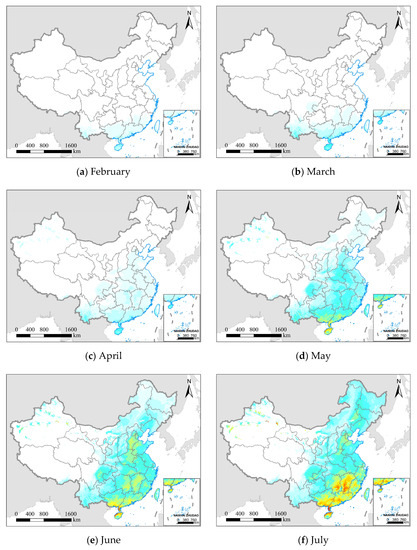
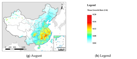
Figure 8.
The mean daily growth rate (environmental suitability) of FAW from February to August 2020; (a–g) represent different months; the white areas represent areas that are not suitable for FAW; and (h) the legend from blue to red represents increased growth rate and environmental suitability.
The distribution of FAW (Figure 5) usually shows a lag compared with the suitable environment (Figure 8). FAW spread to central China in May, while the suitable environment area had extended to northern China. Not all areas with suitable environments and available hosts will be threatened by FAW. In the Northwest China Inland maize region, even from June to August when both environment and hosts were suitable, the possibility of crops damaged by FAW was low due to poor geographical connectivity with existing FAW areas and the lack of favorable seasonal wind flow. This was also the reason for further refining the spatial extent of pest dispersal using the insect migration simulation module in this research. The environmental suitability continued to increase from February to July, and began to decrease in August at mid-latitudes (Figure S5). This is consistent with the results of [17], which showed that the migration of FAW in China has a pronounced northward migration trend before August, and part of the FAW’s return journey to the south began in September.
When encountering downdrafts, cold air, or rain, insects may be forced to terminate migrations, and their density decreases significantly after moderate to heavy rainfall [80]. The locations of summer rainfall belts in eastern China are controlled by the Western Pacific Subtropical High Pressure (WPSH). From April, the WPSH moves northward, so that the impact range gradually moves northward from southern China to the middle and lower reaches of the Yangtze River plain, and a Meiyu belt forms from June to July, bringing continuous rainfall [81]. In this study, we considered the forced landing behavior of FAW in response to rainfall during migration. The results are consistent with the seasonal movement of WPSH, with a single peak trend of increasing and then decreasing effect of rainfall on FAW migration from February to August. The effect of rainfall on FAW migration was greatest during the rainy season of May–July.
The average RIP of maize phenology was the lowest, which is because the host plant is also influenced by the environment, and its phenology is a reflection of environmental conditions and human factors. According to the analysis of data collected by FAO FAMEWS Global Platform (https://www.fao.org/fall-armyworm/monitoring-tools/famews-global-platform/en/, accessed on 20 April 2022) in Africa, many FAW infestations were recorded in the vegetative and reproductive stages of maize. In Kenya, FAW populations increased as the maize planting season began, with two peaks in FAW abundance that coincided with the local crop seasons [82]. The initial infestation of FAW occurred as early as the three- to four-leaf stage of maize [22]. When the crop was almost mature, the number of larvae and adults in the field decreased sharply, which was consistent with the parameters set in this study. The FAW dynamic distribution model used in this study only considered maize as the main host crop, based on the survey report that maize is the most severely infested crop in China (98.1% of the total infested area) [14,83]. However, FAW is a polyphagous pest that can infest at least 353 plants [84,85]. The incomplete consideration of host plants may lead to the underestimation of the prediction results of the suitable spatial range of FAW. In the future, more refined modeling should be developed for thorough consideration of the effects of host plants on the FAW.
5. Conclusions
Based on remote sensing data and meteorological assimilation products, this study examined the impact of migration, host plants, and the environment on the life history of FAW, developed a process-explicit dynamic spatial distribution model of the FAW (FAW-DDM), and the potential spatial distribution of FAW in China from February to August 2020 was simulated. The results showed a significant linear relationship between the first simulated invasion dates and the first observed invasion dates of FAW in 125 cities (R2 = 0.623; p < 0.001). The influencing factors affecting the distribution of FAW were analyzed by month. Environmental factors including air temperature and soil water content were the main influencing factors from February to April, with an average RIP of 85.8%. From May to July with the onset of the rainy season, the influence of precipitation dominated, with an average RIP of 60.32%. In mid to late August, the main growing season in the main maize planting areas came to an end, and maize phenology became the main influencing factor with 62.72% of RIP. According to the spatial distribution characteristics of FAW in China, its northward migration is divided into three periods, namely the overwintering breeding period, the transitional migration period, and the key preventive period. The regions of focus and the prevention and control strategies implemented can be adjusted according to the spatial and temporal distribution of FAW. The results of this study can provide data support for precise control of FAW, which can help integrated management of FAW, and reduce its impact on food security.
Supplementary Materials
The following supporting information can be downloaded at: https://www.mdpi.com/article/10.3390/rs14174415/s1, Figure S1: The starting points of the fall armyworm’s migration every night in February 2020; Figure S2: Simulation results of the temperature-dependent model of fall armyworm; Figure S3: Monthly average 2 m temperature from January to August 2020; Figure S4: Monthly total precipitation from January to August 2020; Figure S5: The monthly mean daily growth rate (environmental suitability) of FAW by (a) longitude, (b) latitude from January to August 2020; Table S1: The first observed invasion dates (week no.) and first simulated invasion dates (week no.) of fall armyworm in 125 cities in China; Table S2: Developmental parameters for fall armyworm; Table S3: Probability density of FAW landing points by province for February–August 2020.
Author Contributions
Conceptualization, Y.H., H.L. and Y.D.; methodology, Y.H., H.L. and H.C.; data curation, Y.H. and H.L.; software, Y.H., H.L. and G.H.; validation, Y.H. and Y.D.; formal analysis, Y.H., H.L. and Y.L.; writing—original draft preparation, Y.H.; writing—review and editing, Y.D., W.H., G.H., J.B., Y.G. and P.G.; visualization, Y.H. and Y.C.; supervision, W.H., Y.D. and G.H.; project administration, W.H. and Y.D.; funding acquisition, W.H. and Y.D. All authors have read and agreed to the published version of the manuscript.
Funding
This research was funded by National Key R & D Program of China (2021YFE0194800); the National Natural Science Foundation of China (42071320); International Partnership Program of Chinese Academy of Science (Grant No. 183611KYSB20200080); Alliance of International Science Organizations (Grant No. ANSO-CR-KP-2021-06); and SINO-EU, Dragon 5 proposal: Application of Sino-Eu Optical Data into Agronomic Models to Predict Crop Performance and to Monitor and Forecast Crop Pests and Diseases (ID 57457).
Data Availability Statement
All the data used in this study are available publicly. The Final Analysis data are available from NCEP (https://rda.ucar.edu/datasets/ds083.2/, accessed on 10 February 2022); the Digital Elevation Models (DEM) are available from USGS (https://www.usgs.gov/centers/eros/science/usgs-eros-archive-digital-elevation-global-multi-resolution-terrain-elevation, accessed on 16 February 2022); the ERA5-Land data products are available from Copernicus Climate Change Service (C3S) Climate Data Store (CDS) (https://cds.climate.copernicus.eu/cdsapp#!/dataset/reanalysis-era5-land?tab = overview; accessed on 10 February 2022); the ChinaCropPhen1km dataset is available from https://doi.org/10.6084/m9.figshare.8313530 (accessed on 25 October 2021).
Acknowledgments
The authors would like to sincerely thank James Maino from Cesar/University of Melbourne for his valuable guidance. We are grateful to the academic editor and reviewers for their insightful comments, which greatly helped us improve the quality of this manuscript.
Conflicts of Interest
The authors declare no conflict of interest.
References
- Chapman, J.W.; Reynolds, D.R.; Wilson, K. Long-Range Seasonal Migration in Insects: Mechanisms, Evolutionary Drivers and Ecological Consequences. Ecol. Lett. 2015, 18, 287–302. [Google Scholar] [CrossRef] [PubMed]
- Satterfield, D.A.; Sillett, T.S.; Chapman, J.W.; Altizer, S.; Marra, P.P. Seasonal Insect Migrations: Massive, Influential, and Overlooked. Front. Ecol. Environ. 2020, 18, 335–344. [Google Scholar] [CrossRef]
- Coutinho-Silva, R.D.; Montes, M.A.; Oliveira, G.F.; de Carvalho-Neto, F.G.; Rohde, C.; Garcia, A.C.L. Effects of Seasonality on Drosophilids (Insecta, Diptera) in the Northern Part of the Atlantic Forest, Brazil. Bull. Entomol. Res. 2017, 107, 634–644. [Google Scholar] [CrossRef] [PubMed]
- Lovett, G.M.; Weiss, M.; Liebhold, A.M.; Holmes, T.P.; Leung, B.; Lambert, K.F.; Orwig, D.A.; Campbell, F.T.; Rosenthal, J.; McCullough, D.G.; et al. Nonnative Forest Insects and Pathogens in the United States: Impacts and Policy Options. Ecol. Appl. 2016, 26, 1437–1455. [Google Scholar] [CrossRef]
- Overton, K.; Maino, J.L.; Day, R.; Umina, P.A.; Bett, B.; Carnovale, D.; Ekesi, S.; Meagher, R.; Reynolds, O.L. Global Crop Impacts, Yield Losses and Action Thresholds for Fall Armyworm (Spodoptera Frugiperda): A Review. Crop Prot. 2021, 145, 105641. [Google Scholar] [CrossRef]
- FAO Global Action for Fall Armyworm Control. Available online: https://www.fao.org/fall-armyworm/monitoring-tools/faw-map/en/ (accessed on 14 January 2022).
- Luginbill, P. The Fall Army Worm; U.S. Department of Agriculture: Washington, DC, USA, 1928. [Google Scholar]
- Nagoshi, R.N.; Meagher, R.L.; Hay-Roe, M. Inferring the Annual Migration Patterns of Fall Armyworm (Lepidoptera: Noctuidae) in the United States from Mitochondrial Haplotypes. Ecol. Evol. 2012, 2, 1458–1467. [Google Scholar] [CrossRef]
- Pair, S.D.; Raulston, J.R.; Westbrook, J.K.; Wolf, W.W.; Adams, S.D. Fall Armyworm (Lepidoptera: Noctuidae) Outbreak Originating in the Lower Rio Grande Valley, 1989. Fla. Entomol. 1991, 74, 200–213. [Google Scholar] [CrossRef]
- Mitchell, E.R.; McNeil, J.N.; Westbrook, J.K.; Silvain, J.F.; Lalanne-Cassou, B.; Chalfant, R.B.; Pair, S.D.; Waddill, V.H.; Sotomayor-Rios, A.; Proshold, F.I. Seasonal Periodicity of Fall Armyworm, (Lepidoptera: Noctuidae) in the Caribbean Basin and Northward to Canada. J. Entomol. Sci. 1991, 26, 39–50. [Google Scholar] [CrossRef]
- Walter, J.A.; Ives, A.R.; Tooker, J.F.; Johnson, D.M. Life History and Habitat Explain Variation among Insect Pest Populations Subject to Global Change. Ecosphere 2018, 9, e02274. [Google Scholar] [CrossRef]
- Ramos, R.S.; Kumar, L.; Shabani, F.; da Silva, R.S.; de Araújo, T.A.; Picanço, M.C. Climate Model for Seasonal Variation in Bemisia Tabaci Using CLIMEX in Tomato Crops. Int. J. Biometeorol. 2019, 63, 281–291. [Google Scholar] [CrossRef]
- Zhang, D.; Xiao, Y.; Xu, P.; Yang, X.; Wu, Q.; Wu, K. Insecticide Resistance Monitoring for the Invasive Populations of Fall Armyworm, Spodoptera Frugiperda in China. J. Integr. Agric. 2021, 20, 783–791. [Google Scholar] [CrossRef]
- Zhou, Y.; Wu, Q.; Zhang, H.; Wu, K. Spread of Invasive Migratory Pest Spodoptera Frugiperda and Management Practices throughout China. J. Integr. Agric. 2021, 20, 637–645. [Google Scholar] [CrossRef]
- Li, X.; Wu, M.; Ma, J.; Gao, B.; Wu, Q.; Chen, A.; Liu, J.; Jiang, Y.; Zhai, B.; Early, R.; et al. Prediction of Migratory Routes of the Invasive Fall Armyworm in Eastern China Using a Trajectory Analytical Approach. Pest. Manag. Sci. 2020, 76, 454–463. [Google Scholar] [CrossRef] [PubMed]
- Jia, H.; Guo, J.; Wu, Q.; Hu, C.; Li, X.; Zhou, X.; Wu, K. Migration of Invasive Spodoptera Frugiperda (Lepidoptera: Noctuidae) across the Bohai Sea in Northern China. J. Integr. Agric. 2021, 20, 685–693. [Google Scholar] [CrossRef]
- Wu, Q.; Jiang, Y.; Liu, J.; Hu, G.; Wu, K. Trajectory Modeling Revealed a Southwest-Northeast Migration Corridor for Fall Armyworm Spodoptera Frugiperda (Lepidoptera: Noctuidae) Emerging from the North China Plain. Insect Sci. 2021, 28, 649–661. [Google Scholar] [CrossRef] [PubMed]
- Zhou, X.; Wu, Q.; Jia, H.; Wu, K. Searchlight Trapping Reveals Seasonal Cross-Ocean Migration of Fall Armyworm over the South China Sea. J. Integr. Agric. 2021, 20, 673–684. [Google Scholar] [CrossRef]
- Early, R.; González-Moreno, P.; Murphy, S.T.; Day, R. Forecasting the Global Extent of Invasion of the Cereal Pest Spodoptera Frugiperda, the Fall Armyworm. NeoBiota 2018, 40, 25–50. [Google Scholar] [CrossRef]
- Norberg, A.; Abrego, N.; Blanchet, F.G.; Adler, F.R.; Anderson, B.J.; Anttila, J.; Araújo, M.B.; Dallas, T.; Dunson, D.; Elith, J.; et al. A Comprehensive Evaluation of Predictive Performance of 33 Species Distribution Models at Species and Community Levels. Ecol. Monogr. 2019, 89, e01370. [Google Scholar] [CrossRef]
- Ramasamy, M.; Das, B.; Ramesh, R. Predicting Climate Change Impacts on Potential Worldwide Distribution of Fall Armyworm Based on CMIP6 Projections. J. Pest. Sci. 2022, 95, 841–854. [Google Scholar] [CrossRef]
- Westbrook, J.K.; Nagoshi, R.N.; Meagher, R.L.; Fleischer, S.J.; Jairam, S. Modeling Seasonal Migration of Fall Armyworm Moths. Int. J. Biometeorol. 2016, 60, 255–267. [Google Scholar] [CrossRef]
- Wu, Q.; Hu, G.; Westbrook, J.K.; Sword, G.A.; Zhai, B. An Advanced Numerical Trajectory Model Tracks a Corn Earworm Moth Migration Event in Texas, USA. Insects 2018, 9, 115. [Google Scholar] [CrossRef] [PubMed]
- Guillera-Arroita, G. Modelling of Species Distributions, Range Dynamics and Communities under Imperfect Detection: Advances, Challenges and Opportunities. Ecography 2017, 40, 281–295. [Google Scholar] [CrossRef]
- Sun, R.; Huang, W.; Dong, Y.; Zhao, L.; Zhang, B.; Ma, H.; Geng, Y.; Ruan, C.; Xing, N.; Chen, X.; et al. Dynamic Forecast of Desert Locust Presence Using Machine Learning with a Multivariate Time Lag Sliding Window Technique. Remote Sens. 2022, 14, 747. [Google Scholar] [CrossRef]
- Barker, B.S.; Coop, L.; Wepprich, T.; Grevstad, F.; Cook, G. DDRP: Real-Time Phenology and Climatic Suitability Modeling of Invasive Insects. PLoS ONE 2020, 15, e0244005. [Google Scholar] [CrossRef]
- Briscoe, N.J.; Elith, J.; Salguero-Gómez, R.; Lahoz-Monfort, J.J.; Camac, J.S.; Giljohann, K.M.; Holden, M.H.; Hradsky, B.A.; Kearney, M.R.; McMahon, S.M.; et al. Forecasting Species Range Dynamics with Process-Explicit Models: Matching Methods to Applications. Ecol. Lett. 2019, 22, 1940–1956. [Google Scholar] [CrossRef]
- Rhodes, M.W.; Bennie, J.J.; Spalding, A.; ffrench-Constant, R.H.; Maclean, I.M.D. Recent Advances in the Remote Sensing of Insects. Biol. Rev. 2022, 97, 343–360. [Google Scholar] [CrossRef]
- Blum, M.; Lensky, I.M.; Rempoulakis, P.; Nestel, D. Modeling Insect Population Fluctuations with Satellite Land Surface Temperature. Ecol. Model. 2015, 311, 39–47. [Google Scholar] [CrossRef]
- Azrag, A.G.A.; Pirk, C.W.W.; Yusuf, A.A.; Pinard, F.; Niassy, S.; Mosomtai, G.; Babin, R. Prediction of Insect Pest Distribution as Influenced by Elevation: Combining Field Observations and Temperature-Dependent Development Models for the Coffee Stink Bug, Antestiopsis Thunbergii (Gmelin). PLoS ONE 2018, 13, e0199569. [Google Scholar] [CrossRef]
- Bae, S.; Müller, J.; Förster, B.; Hilmers, T.; Hochrein, S.; Jacobs, M.; Leroy, B.M.L.; Pretzsch, H.; Weisser, W.W.; Mitesser, O. Tracking the Temporal Dynamics of Insect Defoliation by High-Resolution Radar Satellite Data. Methods Ecol. Evol. 2022, 13, 121–132. [Google Scholar] [CrossRef]
- Wu, B.; Gommes, R.; Zhang, M.; Zeng, H.; Yan, N.; Zou, W.; Zheng, Y.; Zhang, N.; Chang, S.; Xing, Q.; et al. Global Crop Monitoring: A Satellite-Based Hierarchical Approach. Remote Sens. 2015, 7, 3907–3933. [Google Scholar] [CrossRef] [Green Version]
- Lembrechts, J.J.; Lenoir, J.; Roth, N.; Hattab, T.; Milbau, A.; Haider, S.; Pellissier, L.; Pauchard, A.; Ratier Backes, A.; Dimarco, R.D.; et al. Comparing Temperature Data Sources for Use in Species Distribution Models: From in-Situ Logging to Remote Sensing. Glob. Ecol. Biogeogr. 2019, 28, 1578–1596. [Google Scholar] [CrossRef]
- Benami, E.; Jin, Z.; Carter, M.R.; Ghosh, A.; Hijmans, R.J.; Hobbs, A.; Kenduiywo, B.; Lobell, D.B. Uniting Remote Sensing, Crop Modelling and Economics for Agricultural Risk Management. Nat. Rev. Earth Env. 2021, 2, 140–159. [Google Scholar] [CrossRef]
- Yang, X.; Song, Y.; Sun, X.; Shen, X.; Wu, Q.; Zhang, H.; Zhang, D.; Zhao, S.; Liang, G.; Wu, K. Population Occurrence of the Fall Armyworm, Spodoptera Frugiperda (Lepidoptera: Noctuidae), in the Winter Season of China. J. Integr. Agric. 2021, 20, 772–782. [Google Scholar] [CrossRef]
- Zhao, J.; Yang, X. Distribution of High-Yield and High-Yield-Stability Zones for Maize Yield Potential in the Main Growing Regions in China. Agric. For. Meteorol. 2018, 248, 511–517. [Google Scholar] [CrossRef]
- USGS GMTED2010|U.S. Geological Survey. Available online: https://www.usgs.gov/coastal-changes-and-impacts/gmted2010 (accessed on 16 February 2022).
- NECP; NCEP; FNL. Operational Model Global Tropospheric Analyses, Continuing from July 1999. Available online: https://rda.ucar.edu/datasets/ds083.2/ (accessed on 10 February 2022).
- Skamarock, W.C.; Klemp, J.B.; Dudhia, J.; Gill, D.O.; Liu, Z.; Berner, J.; Wang, W.; Powers, J.G.; Duda, M.G.; Barker, D.M.; et al. A Description of the Advanced Research WRF Model Version 4; UCAR/NCAR: Boulder, CO, USA, 2019. [Google Scholar]
- Ma, J.; Wang, Y.; Wu, M.; Gao, B.; Liu, J.; Lee, G.; Otuka, A.; Hu, G. High Risk of the Fall Armyworm Invading Japan and the Korean Peninsula via Overseas Migration. J. Appl. Entomol. 2019, 143, 911–920. [Google Scholar] [CrossRef]
- Liang, S.; Cheng, J.; Jia, K.; Jiang, B.; Liu, Q.; Xiao, Z.; Yao, Y.; Yuan, W.; Zhang, X.; Zhao, X.; et al. The Global Land Surface Satellite (GLASS) Product Suite. Bull. Am. Meteorol. Soc. 2021, 102, E323–E337. [Google Scholar] [CrossRef]
- Liang, S.; Zhao, X.; Liu, S.; Yuan, W.; Cheng, X.; Xiao, Z.; Zhang, X.; Liu, Q.; Cheng, J.; Tang, H.; et al. A Long-Term Global LAnd Surface Satellite (GLASS) Data-Set for Environmental Studies. Int. J. Digit. Earth 2013, 6, 5–33. [Google Scholar] [CrossRef]
- Liu, J.; Kuang, W.; Zhang, Z.; Xu, X.; Qin, Y.; Ning, J.; Zhou, W.; Zhang, S.; Li, R.; Yan, C.; et al. Spatiotemporal Characteristics, Patterns, and Causes of Land-Use Changes in China since the Late 1980s. J. Geogr. Sci. 2014, 24, 195–210. [Google Scholar] [CrossRef]
- Muñoz-Sabater, J.; Dutra, E.; Agustí-Panareda, A.; Albergel, C.; Arduini, G.; Balsamo, G.; Boussetta, S.; Choulga, M.; Harrigan, S.; Hersbach, H.; et al. ERA5-Land: A State-of-the-Art Global Reanalysis Dataset for Land Applications. Earth Syst. Sci. Data 2021, 13, 4349–4383. [Google Scholar] [CrossRef]
- Ayra-Pardo, C.; Borras-Hidalgo, O. Fall Armyworm (FAW.; Lepidoptera: Noctuidae): Moth Oviposition and Crop Protection. In Olfactory Concepts of Insect Control—Alternative to Insecticides: Volume 1; Picimbon, J.-F., Ed.; Springer International Publishing: Cham, Switzerland, 2019; pp. 93–116. ISBN 978-3-030-05060-3. [Google Scholar]
- FAO. Integrated Management of the Fall Armyworm on Maize: A Guide for Farmer Field Schools in Afica; FAO: Rome, Italy, 2018. [Google Scholar]
- Ciampitti, I.; Elmore, R.; Lauer, J. New Corn Growth and Development Poster from K-State. Available online: https://webapp.agron.ksu.edu/agr_social/m_eu_article.throck?article_id=1010 (accessed on 11 March 2022).
- Hu, G.; Lu, F.; Lu, M.; Liu, W.; Xu, W.; Jiang, X.; Zhai, B. The Influence of Typhoon Khanun on the Return Migration of Nilaparvata Lugens (Stål) in Eastern China. PLoS ONE 2013, 8, e57277. [Google Scholar] [CrossRef] [Green Version]
- Chen, H.; Mingfei, W.; Liu, J.; Aidong, C.; Jiang, Y.; Hu, G. Migratory routes and occurrence divisions of the fall armyworm Spodoptera frugiperda in China. J. Plant Prot. 2020, 47, 747–757. [Google Scholar] [CrossRef]
- Ge, S.; He, L.; He, W.; Yan, R.; Wyckhuys, K.A.G.; Wu, K. Laboratory-Based Flight Performance of the Fall Armyworm, Spodoptera frugiperda. J. Integr. Agric. 2021, 20, 707–714. [Google Scholar] [CrossRef]
- Chapman, J.W.; Drake, V.A.; Reynolds, D.R. Recent Insights from Radar Studies of Insect Flight. Annu. Rev. Entomol. 2011, 56, 337–356. [Google Scholar] [CrossRef] [PubMed]
- Wu, M.; Qi, G.; Chen, H.; Ma, J.; Liu, J.; Jiang, Y.; Lee, G.; Otuka, A.; Hu, G. Overseas Immigration of Fall Armyworm, Spodoptera Frugiperda (Lepidoptera: Noctuidae), Invading Korea and Japan in 2019. Insect Sci. 2022, 29, 505–520. [Google Scholar] [CrossRef] [PubMed]
- Qi, G.; Ma, J.; Wan, J.; Ren, Y.; McKirdy, S.; Hu, G.; Zhang, Z. Source Regions of the First Immigration of Fall Armyworm, Spodoptera Frugiperda (Lepidoptera: Noctuidae) Invading Australia. Insects 2021, 12, 1104. [Google Scholar] [CrossRef]
- Zhu, S.; Malmqvist, E.; Li, W.; Jansson, S.; Li, Y.; Duan, Z.; Svanberg, K.; Feng, H.; Song, Z.; Zhao, G.; et al. Insect Abundance over Chinese Rice Fields in Relation to Environmental Parameters, Studied with a Polarization-Sensitive CW near-IR Lidar System. Appl. Phys. B 2017, 123, 211. [Google Scholar] [CrossRef]
- Luo, Y.; Zhang, Z.; Chen, Y.; Li, Z.; Tao, F. ChinaCropPhen1km: A High-Resolution Crop Phenological Dataset for Three Staple Crops in China during 2000–2015 Based on Leaf Area Index (LAI) Products. Earth Syst. Sci. Data 2020, 12, 197–214. [Google Scholar] [CrossRef]
- Sakamoto, T.; Wardlow, B.D.; Gitelson, A.A.; Verma, S.B.; Suyker, A.E.; Arkebauer, T.J. A Two-Step Filtering Approach for Detecting Maize and Soybean Phenology with Time-Series MODIS Data. Remote Sens. Environ. 2010, 114, 2146–2159. [Google Scholar] [CrossRef]
- Sakamoto, T. Refined Shape Model Fitting Methods for Detecting Various Types of Phenological Information on Major U.S. Crops. ISPRS J. Photogramm. Remote Sens. 2018, 138, 176–192. [Google Scholar] [CrossRef]
- Birch, L.C. The Intrinsic Rate of Natural Increase of an Insect Population. J. Anim. Ecol. 1948, 17, 15–26. [Google Scholar] [CrossRef]
- Maino, J.L.; Schouten, R.; Overton, K.; Day, R.; Ekesi, S.; Bett, B.; Barton, M.; Gregg, P.C.; Umina, P.A.; Reynolds, O.L. Regional and Seasonal Activity Predictions for Fall Armyworm in Australia. Curr. Res. Insect Sci. 2021, 1, 100010. [Google Scholar] [CrossRef] [PubMed]
- Schoolfield, R.M.; Sharpe, P.J.H.; Magnuson, C.E. Non-Linear Regression of Biological Temperature-Dependent Rate Models Based on Absolute Reaction-Rate Theory. J. Theor. Biol. 1981, 88, 719–731. [Google Scholar] [CrossRef]
- Barfield, C.S.; Mitchell, E.R.; Poeb, S.L. A Temperature-Dependent Model for Fall Armyworm Development1,2. Ann. Entomol. Soc. Am. 1978, 71, 70–74. [Google Scholar] [CrossRef]
- Ramirez-Cabral, N.Y.Z.; Kumar, L.; Shabani, F. Future Climate Scenarios Project a Decrease in the Risk of Fall Armyworm Outbreaks. J. Agric. Sci. 2017, 155, 1219–1238. [Google Scholar] [CrossRef]
- Ali, A.; Luttrell, R.G.; Schneider, J.C. Effects of Temperature and Larval Diet on Development of the Fall Armyworm (Lepidoptera: Noctuidae). Ann. Entomol. Soc. Am. 1990, 83, 725–733. [Google Scholar] [CrossRef]
- Du Plessis, H.; Schlemmer, M.L.; Van den Berg, J. The Effect of Temperature on the Development of Spodoptera Frugiperda (Lepidoptera: Noctuidae). Insects 2020, 11, 228. [Google Scholar] [CrossRef]
- Valdez-Torres, J.B.; Soto-Landeros, F.; Osuna-Enciso, T.; Báez-Sañudo, M.A. Modelos de predicción fenológica para maíz blanco (Zea mays L.) y gusano cogollero (Spodoptera frugiperda J. E. Smith). Agrociencia 2012, 46, 399–410. [Google Scholar]
- Ge, S.; He, W.; He, L.; Yan, R.; Zhang, H.; Wu, K. Flight Activity Promotes Reproductive Processes in the Fall Armyworm, Spodoptera Frugiperda. J. Integr. Agric. 2021, 20, 727–735. [Google Scholar] [CrossRef]
- Kumela, T.; Simiyu, J.; Sisay, B.; Likhayo, P.; Mendesil, E.; Gohole, L.; Tefera, T. Farmers’ Knowledge, Perceptions, and Management Practices of the New Invasive Pest, Fall Armyworm (Spodoptera Frugiperda) in Ethiopia and Kenya. Int. J. Pest. Manag. 2019, 65, 1–9. [Google Scholar] [CrossRef]
- Allen, M.; Poggiali, D.; Whitaker, K.; Marshall, T.R.; Kievit, R.A. Raincloud Plots: A Multi-Platform Tool for Robust Data Visualization. Wellcome Open Res 2019, 4, 63. [Google Scholar] [CrossRef]
- Zhang, L.; Liu, B.; Zheng, W.; Liu, C.; Zhang, D.; Zhao, S.; Li, Z.; Xu, P.; Wilson, K.; Withers, A.; et al. Genetic Structure and Insecticide Resistance Characteristics of Fall Armyworm Populations Invading China. Mol. Ecol. Resour. 2020, 20, 1682–1696. [Google Scholar] [CrossRef] [PubMed]
- Zidon, R.; Tsueda, H.; Morin, E.; Morin, S. Projecting Pest Population Dynamics under Global Warming: The Combined Effect of Inter- and Intra-Annual Variations. Ecol. Appl. 2016, 26, 1198–1210. [Google Scholar] [CrossRef] [PubMed]
- Sun, X.; Hu, C.; Jia, H.; Wu, Q.; Shen, X.; Zhao, S.; Jiang, Y.; Wu, K. Case Study on the First Immigration of Fall Armyworm, Spodoptera Frugiperda Invading into China. J. Integr. Agric. 2021, 20, 664–672. [Google Scholar] [CrossRef]
- Fand, B.B.; Tonnang, H.E.Z.; Kumar, M.; Kamble, A.L.; Bal, S.K. A Temperature-Based Phenology Model for Predicting Development, Survival and Population Growth Potential of the Mealybug, Phenacoccus Solenopsis Tinsley (Hemiptera: Pseudococcidae). Crop Prot. 2014, 55, 98–108. [Google Scholar] [CrossRef]
- Rebaudo, F.; Rabhi, V.B. Modeling Temperature-Dependent Development Rate and Phenology in Insects: Review of Major Developments, Challenges, and Future Directions. Entomol. Exp. Appl. 2018, 166, 607–617. [Google Scholar] [CrossRef]
- He, L.; Zhao, S.; Ali, A.; Ge, S.; Wu, K. Ambient Humidity Affects Development, Survival, and Reproduction of the Invasive Fall Armyworm, Spodoptera Frugiperda (Lepidoptera: Noctuidae), in China. J. Econ. Entomol. 2021, 114, 1145–1158. [Google Scholar] [CrossRef] [PubMed]
- Meentemeyer, R.K.; Cunniffe, N.J.; Cook, A.R.; Filipe, J.A.N.; Hunter, R.D.; Rizzo, D.M.; Gilligan, C.A. Epidemiological Modeling of Invasion in Heterogeneous Landscapes: Spread of Sudden Oak Death in California (1990–2030). Ecosphere 2011, 2, art17. [Google Scholar] [CrossRef]
- Bale, J.S.; Masters, G.J.; Hodkinson, I.D.; Awmack, C.; Bezemer, T.M.; Brown, V.K.; Butterfield, J.; Buse, A.; Coulson, J.C.; Farrar, J.; et al. Herbivory in Global Climate Change Research: Direct Effects of Rising Temperature on Insect Herbivores. Glob. Chang. Biol. 2002, 8, 1–16. [Google Scholar] [CrossRef]
- Zhang, R.; Qi, J.; Leng, S.; Wang, Q. Long-Term Vegetation Phenology Changes and Responses to Preseason Temperature and Precipitation in Northern China. Remote Sens. 2022, 14, 1396. [Google Scholar] [CrossRef]
- Zeng, L.; Wardlow, B.D.; Xiang, D.; Hu, S.; Li, D. A Review of Vegetation Phenological Metrics Extraction Using Time-Series, Multispectral Satellite Data. Remote Sens. Environ. 2020, 237, 111511. [Google Scholar] [CrossRef]
- Zurell, D.; Thuiller, W.; Pagel, J.; Cabral, J.S.; Münkemüller, T.; Gravel, D.; Dullinger, S.; Normand, S.; Schiffers, K.H.; Moore, K.A.; et al. Benchmarking Novel Approaches for Modelling Species Range Dynamics. Glob. Chang. Biol. 2016, 22, 2651–2664. [Google Scholar] [CrossRef] [Green Version]
- Hu, G.; Lu, M.; Reynolds, D.R.; Wang, H.; Chen, X.; Liu, W.; Zhu, F.; Wu, X.; Xia, F.; Xie, M.; et al. Long-Term Seasonal Forecasting of a Major Migrant Insect Pest: The Brown Planthopper in the Lower Yangtze River Valley. J. Pest. Sci. 2019, 92, 417–428. [Google Scholar] [CrossRef] [PubMed]
- Lu, M.; Chen, X.; Liu, W.; Zhu, F.; Lim, K.; McInerney, C.E.; Hu, G. Swarms of Brown Planthopper Migrate into the Lower Yangtze River Valley under Strong Western Pacific Subtropical Highs. Ecosphere 2017, 8, e01967. [Google Scholar] [CrossRef]
- Niassy, S.; Agbodzavu, M.K.; Kimathi, E.; Mutune, B.; Abdel-Rahman, E.F.M.; Salifu, D.; Hailu, G.; Belayneh, Y.T.; Felege, E.; Tonnang, H.E.Z.; et al. Bioecology of Fall Armyworm Spodoptera Frugiperda (J. E. Smith), Its Management and Potential Patterns of Seasonal Spread in Africa. PLoS ONE 2021, 16, e0249042. [Google Scholar] [CrossRef] [PubMed]
- Ingber, D.A.; McDonald, J.H.; Mason, C.E.; Flexner, L. Oviposition Preferences, Bt Susceptibilities, and Tissue Feeding of Fall Armyworm (Lepidoptera: Noctuidae) Host Strains. Pest Manag. Sci. 2021, 77, 4091–4099. [Google Scholar] [CrossRef]
- Montezano, D.G.; Specht, A.; Sosa-Gómez, D.R.; Roque-Specht, V.F.; Sousa-Silva, J.C.; Paula-Moraes, S.V.; Peterson, J.A.; Hunt, T.E. Host Plants of Spodoptera Frugiperda (Lepidoptera: Noctuidae) in the Americas. Afr. Entomol. 2018, 26, 286–300. [Google Scholar] [CrossRef]
- Wan, J.; Huang, C.; Li, C.; Zhou, H.; Ren, Y.; Li, Z.; Xing, L.; Zhang, B.; Qiao, X.; Liu, B.; et al. Biology, Invasion and Management of the Agricultural Invader: Fall Armyworm, Spodoptera Frugiperda (Lepidoptera: Noctuidae). J. Integr. Agric. 2021, 20, 646–663. [Google Scholar] [CrossRef]
Publisher’s Note: MDPI stays neutral with regard to jurisdictional claims in published maps and institutional affiliations. |
© 2022 by the authors. Licensee MDPI, Basel, Switzerland. This article is an open access article distributed under the terms and conditions of the Creative Commons Attribution (CC BY) license (https://creativecommons.org/licenses/by/4.0/).