Article

Sparse SAR Imaging Method for Ground Moving Target via GMTSI-Net

1
Information and Navigation College, Air Force Engineering University, Xi’an 710077, China
2
Collaborative Innovation Center of Information Sensing and Understanding, Air Force Engineering University, Xi’an 710077, China
3
Jiuquan Satellite Launch Center, Jiuquan 732750, China
*
Author to whom correspondence should be addressed.
Remote Sens. 2022, 14(17), 4404; https://doi.org/10.3390/rs14174404
Submission received: 23 July 2022 / Revised: 29 August 2022 / Accepted: 1 September 2022 / Published: 4 September 2022
(This article belongs to the Special Issue SAR Images Processing and Analysis)

Abstract

:
Ground moving targets (GMT), due to the existence of velocity in range and azimuth direction, will lead to the deviation from their true position and defocus in the azimuth direction during the synthetic aperture radar (SAR) imaging process. To address this problem and compress the amount of echo data, a sparse SAR imaging method for ground moving targets is proposed. Specifically, we first constructed a two-dimensional sparse observation model of the GMT based on matched filter operators. Then, the observation model was solved by a deep network, GMT sparse imaging network (GMTSI-Net), which was mainly obtained by unfolding an iterative soft threshold algorithm (ISTA)-based iterative solution. Furthermore, we designed an adaptive unfolding module in the imaging network to improve the adaptability of the network to the input of echo data with different sampling ratios. The proposed imaging network can achieve faster and more accurate SAR images of ground moving targets under a low sampling ratio and signal-to-noise ratio (SNR). Simulated and measured data experiments were conducted to demonstrate the performance of imaging quality of the proposed method.

Graphical Abstract

1. Introduction

Synthetic aperture radar (SAR), as a kind of all-day, all-weather active high-resolution radar imaging system, has been rapidly developing since its birth [1]. Therefore, SAR has been widely used in the fields of Earth remote sensing, military reconnaissance, and marine survey. With the development of SAR imaging technology, people are no longer satisfied with imaging stationary targets on the ground, but hope that SAR can also image ground moving targets (GMT) [2,3,4]. However, when conventional imaging algorithms for stationary targets are used for moving targets, the result will be defocus and deviation. Therefore, the study of SAR imaging methods for GMT is of great value [5,6].
Traditional imaging methods for ground moving targets are based on estimating the velocity parameters (range and azimuth direction) or Doppler parameters of the moving target (center and rate) [7,8], and then designing the matching filter function to compensate for the phase error or distance migration generated by the ground moving target, so as to achieve the focus of the GMT. In general, GMT imaging methods can be divided into transformation-based methods and optimization-based methods. The transformation-based methods mainly include the Keystone transform method [9,10] and the time-frequency transform method [11,12]. Li et al. [9] use the keystone transform to solve the coupling problem between azimuth and range velocities, thus achieving a focused SAR image under high SNR. The time-frequency method uses transform methods (such as Hough transform, fractional FFT, Radon transform, etc.) to estimate the Doppler modulation and center frequency to construct a reference function to achieve matching filtering processing. Optimization-based methods generally characterize moving target imaging as a problem to solve optimization [13,14,15,16]. Gu [15] proposed a parametric sparse representation method to achieve parameter estimation and imaging under low pulse repetition frequency (PRF) conditions. Chen et al. [16] used the parametric sparse representation approach to solve the phase error compensation function directly, avoiding the estimation of velocity parameters and reducing the number of operations for parameter iteration while improving the imaging quality. Zhang [17] proposed an iterative minimum entropy algorithm (IMEA) based on the extraction of the region of interest (ROI) to achieve the estimation and imaging of moving target parameters. However, the above methods have the following two problems: (1) The transform methods require high integrity of the echo signal and low accuracy of parameter estimation under low SNR conditions, and (2) the optimization methods have large iterative computation and long imaging time, making it difficult to meet the requirements of real-time SAR imaging.
In recent years, the application of compress sensing (CS) theory to SAR imaging has been rapidly developed [18,19,20,21,22]. In general, the number of moving targets in a SAR observation scene is finite, and thus the GMT echo signal satisfies sparsity, which allows the use of CS theory for imaging or parameter estimation of the compressed echo data. Wu [19] proposed a multi-channel SAR imaging framework for moving targets based on CS theory. The method achieves parameter estimation and imaging of moving targets by extracting GMT through sparse decomposition and then estimating the velocities using sparsity as a constraint. Zhang et al. [22] proposed an efficient imaging algorithm for GMT. However, these methods suffer from high computational complexity or low accuracy of parameter estimation.
With the development of deep learning, its application in SAR imaging and interpretation has also received the attention of many scholars at home and abroad [22,23,24,25,26]. Mu et al. [27] proposed a moving target imaging network based on convolutional neural network (CNN), which takes a defocus moving target image as input and learns the focus of the moving target through the network. An imaging method for GMT based on improved U-Net is proposed in [28]. Deep unfolded network (DUN) [29,30] can provide an approach to solving the linear inverse problem by unfolding iterative optimization algorithms. DUN-based SAR imaging methods are proposed to reconstruct SAR images with good quality in [31,32]. Zhao et al. [33] proposed an end-to-end imaging network that enables SAR imaging in larger scenes. However, these methods often require retraining of the network when facing imaging requirements with different downsampled echo signal inputs, which undoubtedly increases the computational expense.
To solve the problems of slow imaging speed and high computational complexity of traditional GMT imaging algorithms, and at the same time improve the imaging performance after compressing the GMT echo signal data, a novel sparse SAR imaging method for GMT via ground moving targets sparse imaging network (GMTSI-Net) is proposed in this paper. Similar to the traditional method of designing the compensation function by estimating the moving target echo moving parameters, the proposed method is to input the Doppler modulation and center frequency and the associated imaging matrix into the imaging network as learnable variables, construct the corresponding labels at the same time, and obtain more accurate Doppler modulation and center frequency and imaging matrix by using the supervised learning of the network. In addition, we designed an adaptive unfolding module to improve imaging performance with different sampling ratio inputs. Firstly, we derived the imaging method for GMT based on constructing an echo signal model. Then, due to the sparsity of moving target echoes, we constructed a two-dimensional sparse observation model, confirm the learnable parameters, and unfold the solution algorithm of the model into a network. When the training of the network is completed, the reconstructed SAR images of GMT can be obtained by inputting the moving target echoes with any sampling ratio. The simulated and measured data experiments show that the proposed method can achieve high-quality SAR-GMT images at different sampling ratios or SNRs.
The rest of this paper is organized as follows. Section 2 establishes the SAR ground moving target echo signal model and provides the imaging algorithm. Section 3 derives the sparse observation model for GMT and constructs the GMTSI-Net. Section 4 provides the results and analysis of the simulated and measured experiments. The conclusion is drawn in Section 5.

2. Imaging Model and Algorithm of SAR-GMT

In this section, we first provide the imaging geometric model of SAR-GMT in Section 2.1 and derive the expression of its echo signal. Then, based on Section 2.1, we deduced the SAR moving target imaging algorithm based on the known velocity or Doppler parameters.

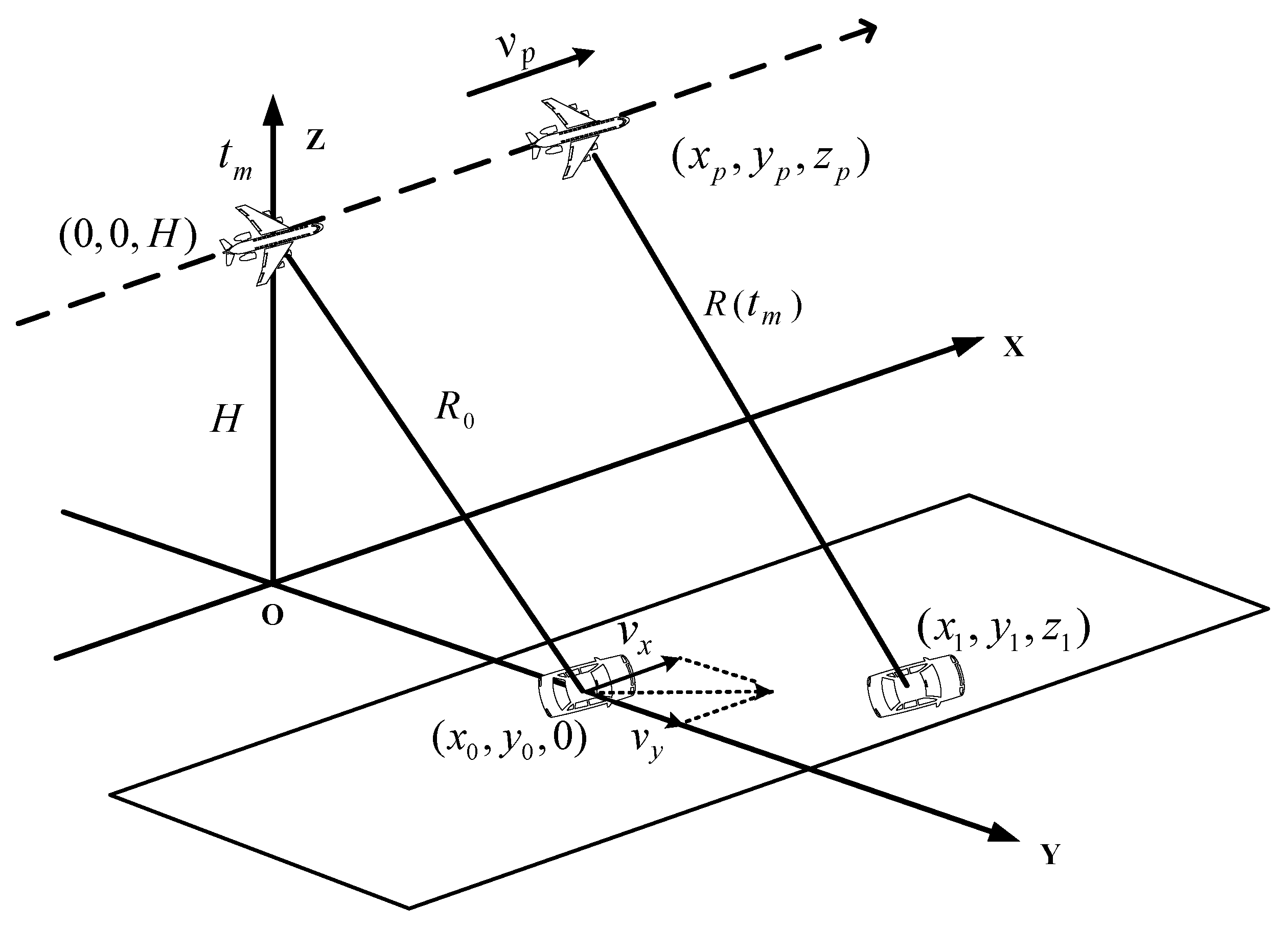
2.1. SAR-GMT Echo Signal Model

Figure 1 shows the geometric relationship between the airborne SAR platform and the GMT. We set the radar imaging system to operate under the positive side-looking and strip map mode. To facilitate the analysis, we considered a single point target in the scene to obtain the general form of the GMT echo signal.
It is assumed that the platform is moving with a uniform velocity v p along the x-axis (azimuth direction) at a height H above the ground and that there is a ground-moving target on the ground whose initial position is at the center of the observation scene with coordinates ( x 0 , y 0 , z 0 ) . The target is moving on the ground with ( v x , v y ) , and v x and v y denote the azimuth and range velocity, respectively. R 0 is the slant range from the platform to the center of the observation scene. t m represents the slow time series, and ( x p , y p , z p ) and ( x 1 , y 1 , z 1 ) denote the instantaneous position of the platform and target, respectively. Then we can get:
R ( t m ) = ( x p - x 1 ) 2 + ( y p - y 1 ) 2 + ( z p - z 1 ) 2
where:
{ x p = v p · t m y p = 0 z p = H { x 1 = x 0 + v x · t m y 1 = y 0 + v y · t m z 1 = 0
Substituting Equation (2) into Equation (1) and expanding R ( t m ) into the Taylor series at t m = 0 achieves:
R ( t m ) = R 0 + R 1 · t m + 1 2 R 2 · t m 2
where:
{ R 0 = x 0 2 + y 0 2 + H 2 R 1 = ( v x - v p ) · x 0 + v y · y 0 R 0 R 2 = [ v y 2 + ( v x - v p ) 2 ] · R 0 2 - [ ( v x - v p ) · x 0 + v y · y 0 ] 2 R 0 3
We can also obtain the Doppler modulation and center frequency of the GMT according to the definition of Doppler as:
{ f d c = 1 λ d ( 2 R ( t m ) ) d t m | t m = 0 = 2 λ x 0 v x + v y y 0 R 0 + 2 λ v p x 0 R 0 = 2 λ R 1 K a = 1 λ d 2 ( 2 R ( t m ) ) d t m 2 | t m = 0 = 2 λ ( v y 2 + ( v x - v p ) 2 R 0 ) = 2 λ R 2
Combined with Equations (5) and (3), this can also be written as:
R ( t m ) = R 0 + R 1 · t m + 1 2 R 2 · t m 2 = R 0 + λ 2 f d c · t m λ 4 K a · t m 2
where f d c and K a denote the Doppler center and modulation frequency of the GMT, respectively.
Assuming that the radar transmits a chirp signal, based on the above analysis, the GMT echo signal received by the SAR platform can be expressed as:
S e c h o ( t k , t m ) = w r ( t k - 2 R ( t m ) c ) · w a ( t m ) · exp [ - j 4 π f c c R ( t m ) ] · exp { j π γ [ t k - 2 R ( t m ) c ] 2 }
where f c is the carrier frequency, t k is the fast time series, c is the speed of the light, and γ is the tuning frequency of the chirp signal. w r and w a represent the envelope of the range and azimuth direction, respectively.

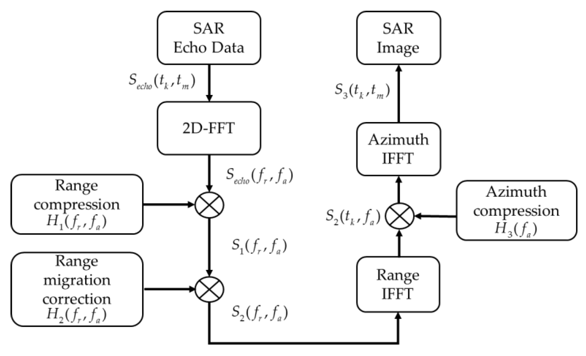
2.2. Traditional SAR-GMT Imaging Method

Through the analysis in Section 2.1, the expression of the SAR-GMT echo signal is obtained. By substituting Equations (3) and (4) into Equation (7) and performing a two-dimensional (2-D) FFT transform (ignoring the envelope of range and azimuth direction), the 2-D frequency domain expression of the echo signal can be written as:
S e c h o ( f r , f a ) = exp [ - j 4 π f r c ( R 0 - R 1 2 2 R 2 ) ] · exp [ - j π f r 2 ( 1 γ - c f a 2 2 R 2 f c 3 ) ] · exp [ j 2 π R 1 R 2 f a ] · exp [ j c π 2 R 2 f c f a 2 ] · exp [ - j c π 2 R 2 f c f a 2 f r ]
where f r and f a denote the frequency domain of range and azimuth direction, respectively. From Equation (8), it can be seen that the moving target leads to the introduction of a new frequency modulation (FM) component of the echo signal in the 2-D frequency domain. Then, we constructed the corresponding range compression function to eliminate the effect of the component, and the specific expression can be written as:
H 1 ( f r , f a ) = exp [ j π f r 2 ( 1 γ c f a 2 2 R 2 f c 3 ) j 4 π f r c R 1 2 2 R 2 ]
Multiplying Equation (9) with Equation (8), we get:
S 1 ( f r , f a ) = S e c h o ( f r , f a ) · H 1 ( f r , f a ) = exp ( j 4 π f r c R 0 ) · exp [ j 2 π R 1 R 2 f a ] · exp [ j c π 2 R 2 f c f a 2 ] · exp [ j c π 2 R 2 f c f a 2 f r ]
It can be seen that there is also a quadratic coupling term in the range and azimuth frequency domain in Equation (10), which will cause the curvature of the range migration curve, so it is necessary to perform a range migration correction on S 1 ( f r , f a ) . Hence, the range migration correction function is given as:
H 2 ( f r , f a ) = exp ( j c π 2 R 2 f c f a 2 f r )
Multiplying Equations (11) and (10) yields:
S 2 ( f r , f a ) = S 1 ( f r , f a ) · H 2 ( f r , f a ) = exp ( j 4 π f r c R 0 ) · exp [ j 2 π R 1 R 2 f a ] · exp [ j c π 2 R 2 f c f a 2 ]
Transforming Equation (12) to the range-Doppler domain yields:
S 2 ( t k , f a ) = IFFT f r { S 2 ( f r , f a ) } = s i n c [ B r ( t k 2 R 0 c ) ] exp [ j 2 π R 1 R 2 f a ] · exp [ j c π 2 R 2 f c f a 2 ]
Since there is a second frequency modulation term in the azimuth direction in Equation (13), it will cause the defocus of the point target. Therefore, the azimuth compression function needs to be constructed, and its expression is given as:
H 3 ( f a ) = exp ( j c π 2 R 2 f c f a 2 ) · exp ( j 2 π R r e f f a )
where R r e f = R 1 / R 2 x 0 . Multiplying Equations (13) and (14) and converting the results back to the time domain yields:
S 3 ( t k , t m ) = IFFT f a { S 2 ( t k , f a ) · H 3 ( f a ) } = s i n c [ B r ( t k 2 R 0 c ) ] · s i n c [ B a ( t m x 0 ) ]
where B r and B a are the signal bandwidth and Doppler bandwidth, respectively. It can be seen from Equation (15) that the moving target is finally focused at ( R 0 , x 0 ) . It is worth noting that the above imaging algorithm requires a known Doppler center and modulation frequency or 2-D velocity of the GMT. The flow of the imaging algorithm is shown in Figure 2.

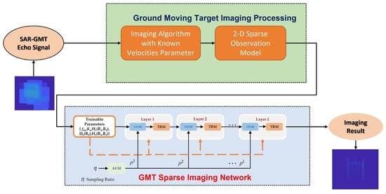
3. Approximate Observation Model and GMTSI-Net for Ground Moving Target

In this section, we derived a 2-D sparse observation model based on the imaging algorithm in Section 2.2 and the sparsity of the GMT echo signal in Section 3.1. Then, we constructed the GMTSI-Net and determine the learnable parameters of the network. This helps the GMT imaging algorithm obtain better imaging performance at a low sampling ratio and SNR.

3.1. 2-D Sparse Observation Model Based on Matched Filter Operators

Since the number of the ground moving targets is limited in the whole observation scene and the echo signals satisfy the sparsity, a 2-D sparse SAR-GMT observation model based on the inversion of the matched filtering algorithm in Section 2.2 can be established.
The algorithm and Figure 2 in Section 2.2 is expressed with a matrix multiplication form as follows:
Ξ G ( S e c h o ) = F a 1 · { [ H 2 ( F a · S e c h o · F r ) H 1 ] · F r 1 H 3 }
where G ( · ) is the imaging operator of the GMT, and Ξ N × M is the result of GMT imaging, i.e., an approximate estimate of the real scattering coefficients. S e c h o N × M is the echo signal of GMT. N and M indicate the sampling points of slow time and fast time, respectively. { H 1 , H 2 , H 3 } N × M are the matrix forms of H 1 ( f r , f a ) , H 2 ( f r , f a ) , and H 3 ( f a ) in Section 2.2, respectively. { F r , F r 1 } M × M are the range FFT and IFFT matrices, respectively, and { F a , F a 1 } N × N are the azimuth FFT and IFFT matrices, respectively. denotes the Hadamard product.
Due to the operation of Equation (16) are all reversible, and the echo of GMT can be gained by the inverse process of Equation (16):
S e c h o   G 1 ( Ξ ) = F a 1 · { H 1 * [ ( F a · Ξ ) H 3 * ] · F r H 2 * } · F r 1
where ( · ) * denotes the conjugate of the matrix. To reduce the amount of echo data, we collected the echo data by random sampling, which is essentially a sampling of the echo at a sampling rate lower than Nyquist’s sampling theorem. The sampling matrix is described by the formula that each column or row vector has only one non-zero element with a value of 1. In addition, the positions of the elements are random. We denote the azimuth and range sampling matrix as Ψ N ^ × N and Φ M × M ^ . The sampling ratios are η 1 = N ^ / N ( N ^ < N ) and η 2 = M ^ / M ( M ^ < M ) , respectively. Then joint sampling ratio is expressed as η = η 1 · η 2 . The specific form is as follows:
Ψ = [ 1 0 0 0 0 0 0 0 1 0 · · · · · · · · · · 0 0 1 0 0 ] N ^ × N Φ = [ 0 0 1 0 0 0 1 0 0 0 · · · · · · · · · · 1 0 0 0 0 ] M × M ^
Then, combining Equations (17) and (18), the downsampled GMT echo signal can be written as:
S d s = Ψ · S e c h o · Φ = Ψ · G 1 ( Ξ ) · Φ
According to the theory of compress sensing, the solution of Equation (19) can be transformed into the following optimization problem:
Ξ ^ = arg min Ξ { 1 2 S d s Ψ G 1 ( Ξ ) Φ 2 2 + χ Ξ p }
where · 2 2 denotes the l2-norm, χ Ξ p is the regularized constraint terms, and χ is the regularization parameter. The effect of this constraint term is to make the reconstruction problem of Equation (20) obtain an optimal solution. Equation (20) is a typical least absolute shrinkage and selection operator (LASSO) problem, which can be obtained by an iterative optimization search with many algorithms (e.g., ISTA, ADMM). Taking the ISTA algorithm as an example [34], the main steps are as follows:
O t = Ξ ^ t 1 + ρ G [ Ψ H ( S d s Ψ G 1 ( Ξ ^ t 1 ) Φ ) Φ H ]
Ξ ^ t = soft ( O t , T ) = sign ( O t ) · max ( | O t | T , 0 )
where O t is the operator after the t -th iteration update, Ξ ^ t 1 is the imaging result of the previous estimation, and ( · ) H represents the transpose operation of a matrix. ρ and T denote the threshold and step size of the iteration, respectively.

3.2. Sparse Imaging Network for Ground Moving Target (GMTSI-Net)

In this subsection, GMTSI-Net is proposed in Section 3.2.1, which takes SAR-GMT echoes as input and outputs a focused SAR image of a moving target. In addition, we give the training strategy of this network in Section 3.2.2.

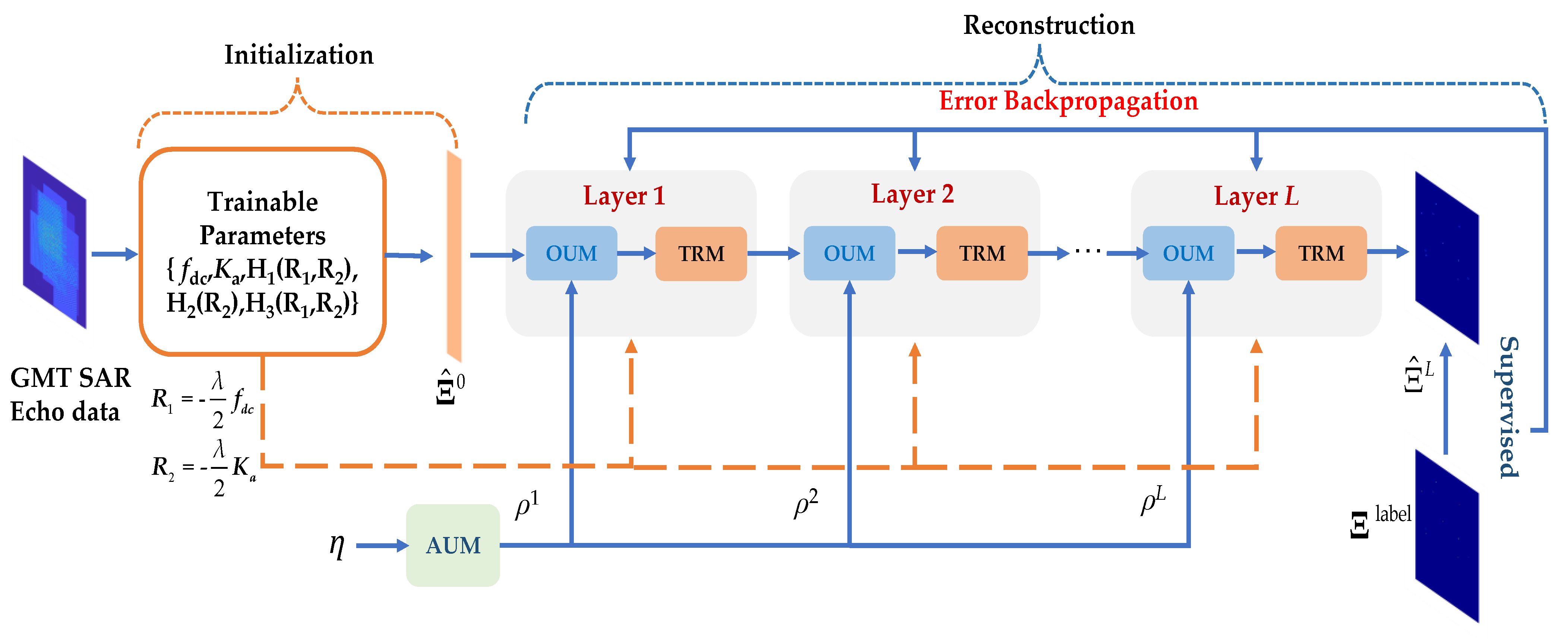
3.2.1. Network Structure

In theory, we can reconstruct the imaging results of GMT focus by iterating Equations (21) and (22) in Section 3.1. However, the Doppler or velocity parameters of the GMT are unknown, and thus the three imaging matrices H 1 , H 2 , and H 3 contained in G in Equation (21) cannot be accurately obtained. Hence, the iterative algorithm of Equations (21) and (22) cannot be effectively applied.
To address the above problems, we propose a ground moving target sparse imaging method that unfolds the ISTA algorithm into a network form. Specifically, the single-layer topology of GMTSI-Net consists of three parts: the Operator Update Module, the Target Reconstruction Module, and the Adaptive Unfolding Module, as described below.
Operator Update Module (OUM): In this module, the main function is to implement Equation (21), where ρ i is the output of the Adaptive Unfolding Module, and then the output of the OUM at the layer i of the network is defined as:
O i = Л OUM i ( Ξ ^ i 1 , ρ i , G , G 1 ) = Ξ ^ i 1 + ρ i G [ Ψ H ( S d s Ψ G 1 ( Ξ ^ i 1 ) Φ ) Φ H ]
Since some parameters (e.g., R 1 , R 2 ) of H 1 , H 2 , and H 3 in G are related to the Doppler center and tuning frequency of the GMT, they can be used as learnable parameters of the GMTSI-Net, labeled as ϒ = { H 1 , H 2 , H 3 , f d c , K a } , where ϒ denotes the set of learnable parameters. It should be noted that in the conventional ISTA algorithm, the value of ρ i is generally fixed in each iteration, whereas in GMSTI-Net, the ρ i is different in each layer of the network and related to the sampling ratio η .
Target Reconstruction Module (TRM): Similar to Equation (22), the function of TRM is mainly to achieve the reconstruction of the GMT and side lobe and noise suppression. The output of TRM is the GMT imaging result, which can be expressed as:
Ξ ^ i = Л TRM i ( O i , T i ) = sign ( O i ) · ReLu ( | O i | T i , 0 )
where T i = λ ρ i , ReLU denotes the Rectified Linear Units activation function.
Adaptive Unfolding Module (AUM): The function of AUM is to enable the GMTSI-Net to adapt to tasks with different sampling ratios and improve imaging performance at the same time. We designed the AUM. AUM uses the sampling ratio η as input and output differently ρ i . We implemented the AUM by setting up two fully connected layers, where the first layer uses ReLU as the activation function and the last uses Softplus, and the number of nodes in each hidden layer is 64. With this design, GMTSI-Net is still able to image GMT at a low sampling ratio. The AUM can be simply written as:
Л AUM ( η ) = { ρ 1 , ρ 2 , , ρ L }
where L denotes the number of network layers.
In GMTSI-Net, each layer of the network contains the same topology, which consists mainly of OUM, TRM, and AUM. To further improve the imaging performance of GMTSI-Net, we constructed the corresponding labels for the supervised training. This training approach allows the network to autonomously learn the non-linear mapping relationship from the GMT echo to the target scattering coefficient. The topology of GMTSI-Net is shown in Figure 3.

3.2.2. Training Strategy

Similar to traditional deep neural networks, the proposed network can be trained in a data-driven error back-propagation manner for end-to-end supervised training.

Loss Function

In general, we can measure the quality of the image reconstruction by the mean square error (MSE). In this paper, the loss function of GMTSI-Net is designed as follows:
L o s s ( ϒ ) = 1 2 N total i = 1 N total ( Ξ ^ i Ξ label 2 2 Ξ label 2 2 + μ 1 Ξ ^ i 1 μ 2 Ξ ^ i 2 2 )
ϒ ^ = argmin ϒ L o s s ( ϒ )
where Ξ ^ i is the output of GMTSI-Net, Ξ label is the label of scattering coefficients, and N total denotes the total number of SAR-GMT echo training samples. μ 1 and μ 2 are the tuning parameters to weigh the MSE against l2 and l1 constraints, respectively. These two constraints are introduced for two purposes: firstly, to ensure convergence of the network parameters, and secondly, to improve the imaging quality under low sampling ratio conditions. In this paper, we set the initial values of μ 1 and μ 2 to be 0.1 and 0.005, respectively. The derivation of the loss function gradient can be found in Appendix A.

Backpropagation and Gradient Update

Similar to a deep neural network, the update of learnable parameters in GMTSI-Net can be implemented by many optimizers, such as SGD, Adagrad, Adam, etc. In this paper, we selected Adam as the optimizer for GMTSI-Net. SAR-GMT echoes are complex data, but in the network the data are propagated as real. We divided the complex data into real and imagery parts to implement the processing of SAR-GMT echo data; the specific method can be found in Ref. [35]. It is worth noting that the network learnable parameters can be updated at each layer, i.e., the value of updated learnable parameters by backpropagation of the network at i -th layer is used as the initial value of the input of i + 1 -th layer. The specific training process is shown in Algorithm 1.
Algorithm 1 Training of GMTSI-Net
Input: Downsampling SAR-GMT echo S d s ; sampling ratio and matrix η ,   Ψ ,   Φ ; number of layers L; imaging labels Ξ label ; learnable parameter set ϒ ; tuning parameters μ 1 ,   μ 2
Output: GMT imaging result Ξ ^
 1: Initialize ϒ 0 = [ f d c 0 , K a 0 , H 1 0 , H 2 0 , H 3 0 ] , Ξ ^ 0 , ε = 1 e 4
 2: for iL do
 3:  Update the operator Oi via OUM
 4:  Estimate the result of GMT imaging Ξ ^ i , and calculate the Loss(ϒ)
 5:   if Loss(ϒ) < ε
 6:    output the result Ξ ^ i
 7:   else
 8:    Update the parameters ϒi + 1 by Equation (27) and Adam optimizer
 9:    i = i + 1
 10: end for

4. Experimental Results and Analysis

In this section, we test the imaging performance of the GMTSI-Net with different SNRs and sampling ratios through simulation and measure data experiments, and compare them with other imaging algorithms to verify the effectiveness and superiority of the proposed method. GMTSI-Net was implemented in the Tensorflow framework and accelerated with an NVIDIA GeForce RTX 3060.
Meanwhile, we used MSE, peak signal-to-noise ratio (PSNR), image entropy (IE), and target-to-background ratio (TBR) as evaluation metrics to measure the imaging results of different algorithms. The related definitions are shown below:
IE = - 1 Μ Ξ ^ m , n ( | Ξ ^ m , n | 2 ln ( | Ξ ^ m , n | 2 ) ) + ln ( Μ Ξ ^ )
TBR = 20 · lg ( Ξ ^ T 2 2 Ξ ^ B 2 2 )
where Μ Ξ ^ = Ξ ^ 2 2 , Ξ ^ m , n indicates the pixel value of the imaging result Ξ ^ at coordinate ( m , n ) . T and B are the region of the target and background, respectively.

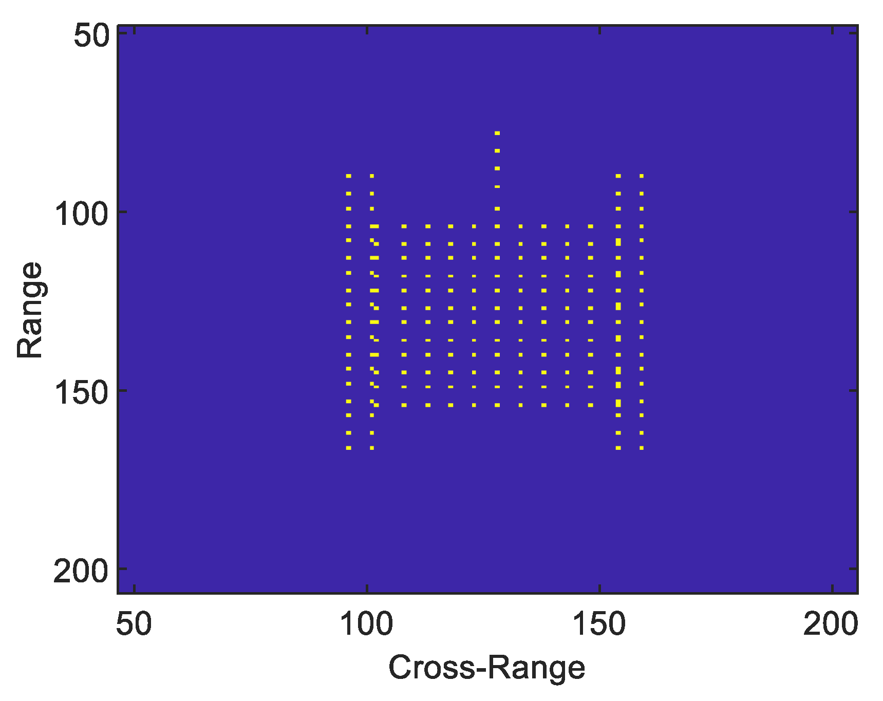
4.1. Point Target Simulation Experiment

In this subsection, we set up a scenario containing 100–300 moving targets. The parameters of the SAR platform were set as follows: the platform traveled at a constant velocity of 100 m/s; the carrier frequency was 10 GHz; the bandwidth was 150 MHz; the pulse repetition frequency and duration were set to 500 Hz and 1.5 μs, respectively; the observation scene size was 256 m × 256 m; and the range and azimuth resolution were both 1 m.
In the process of generating the training set, we generated the training set S G M T E c h o of GMT echoes by randomly sampling the echo signal (sampling ratio between 0.1 and 0.9) and adding Gaussian white noise with a random SNR (SNR between −15 dB and 20 dB). The total number of echo samples was N total = 5000 . Each echo sample consisted of 100–300 moving point targets randomly distributed within the observed scene and their velocities were also random in 2-D directions. The range velocity v y was randomly distributed between 1 m/s and 20 m/s and the azimuth velocity v y was randomly distributed between 5 m/s and 20 m/s. Note that the velocity of moving targets was different in different echo samples, whereas the velocity of moving targets was the same in each echo sample. Note that we only considered differences in moving target velocities between different echo samples and ignored the case where the moving targets in a single echo sample had different velocities. In the initialization of network parameters, the initialization of the learnable parameter set ϒ 0 was set as follows: the Doppler center frequency f d c 0 and Doppler tuning frequency K a 0 were set to −5 and −10, respectively, and the imaging matrices H 1 0 , H 2 0 and H 3 0 were initialized by Equations (9), (11) and (14); the layer of GMTSI-Net was set as L = 12 ; and the learning rate, batch size, and epoch number were set to 2 × e 5 , 32, and 150, respectively.
When testing the network, the trained network parameters were fed into the GMTSI-Net. The imaging results of the moving target were output by a single feed-forward operation of the network. A tank model was chosen to verify the imaging performance of the GMTSI-Net, which consists of 211 independent points with v x = 16 m/s and v y = 8 m/s. Figure 4 shows the schematic diagram of a tank model. We performed simulated experiments under different SNRs and different sampling ratios η to verify the effectiveness and superiority of the proposed method.

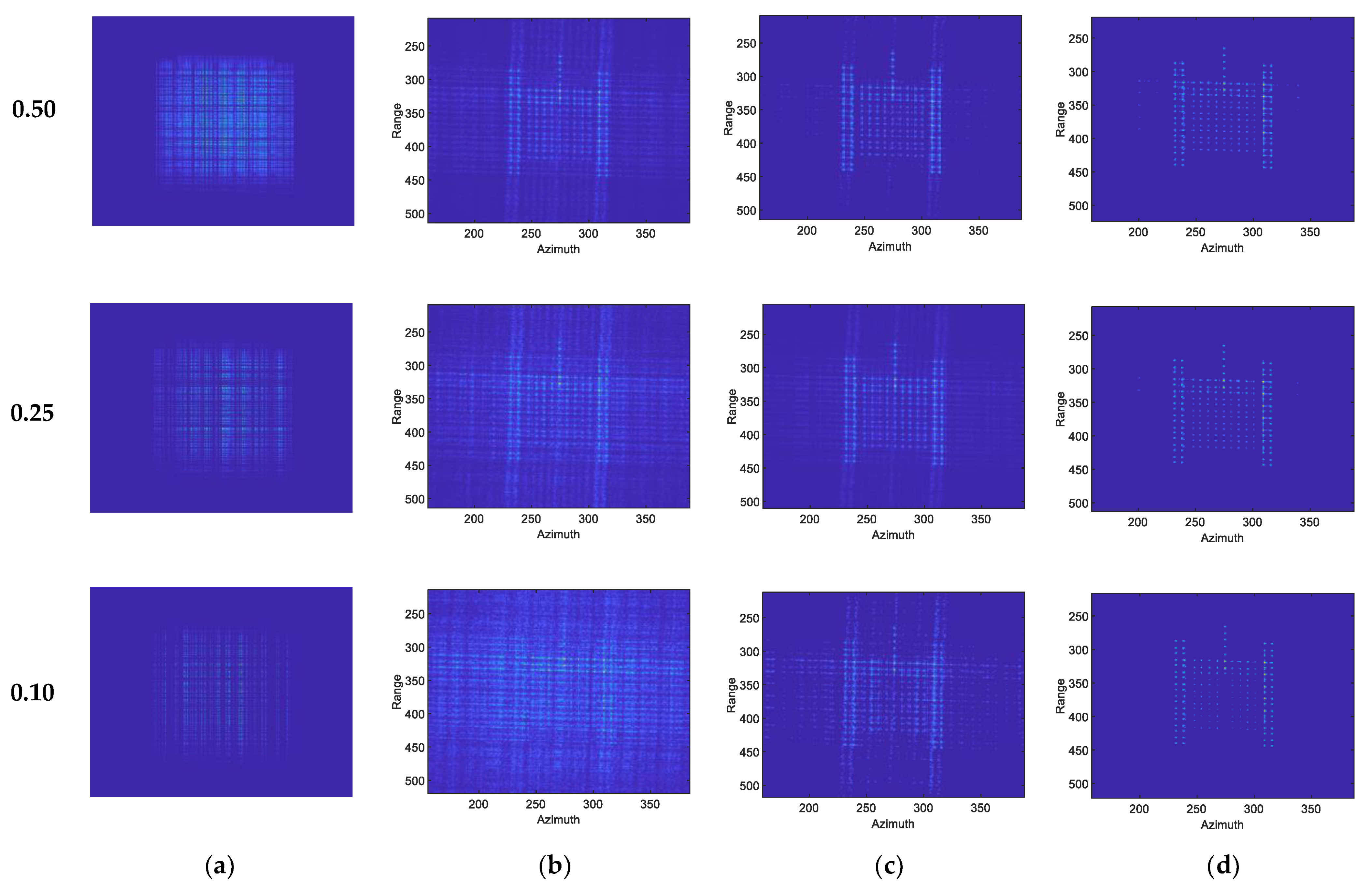
4.1.1. Comparison of Different Sampling Ratios

In this subsubsection, we use the tank model to verify the imaging performance of the proposed method at different sampling ratios of 0.5, 0.25 and 0.1, respectively. The SNR of SAR-GMT was 15 dB.
Figure 5 gives a comparison of the proposed method with other algorithms for different sampling ratios, where the first, second, and last rows show the imaging results for sampling ratio η = 0.5 ,   0.25 ,   and   0.1 , respectively. It can be seen that the method in [8] did not give more accurate imaging results at lower η , and the method in [17] could achieve focused moving targets but had a high side lobe. Besides, the proposed GMTSI-Net effectively focused on the ground-moving targets while achieving the suppression of the side lobe at a low sampling ratio. The proposed method showed a small number of moving targets disappearing at η = 0.1 . The possible reason for this is the influence of the two constraint terms in Equation (26), but the overall outline of the tank model was preserved.
Table 1 gives the values of the evaluation indicators for the three algorithms. GMTSI-Net outperformed the method in [8] and the method in [17] to a relatively large extent in imaging quality and time.

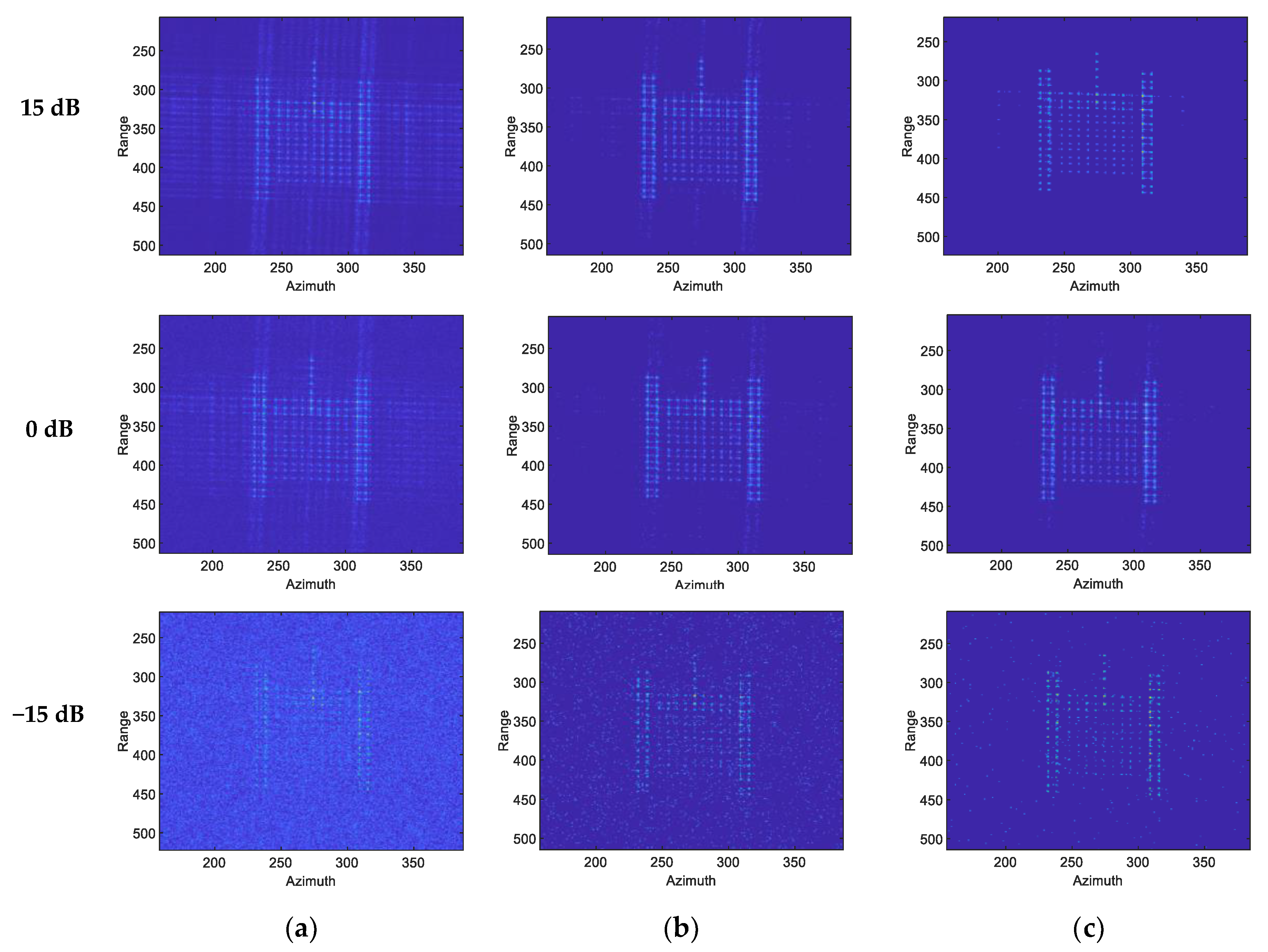
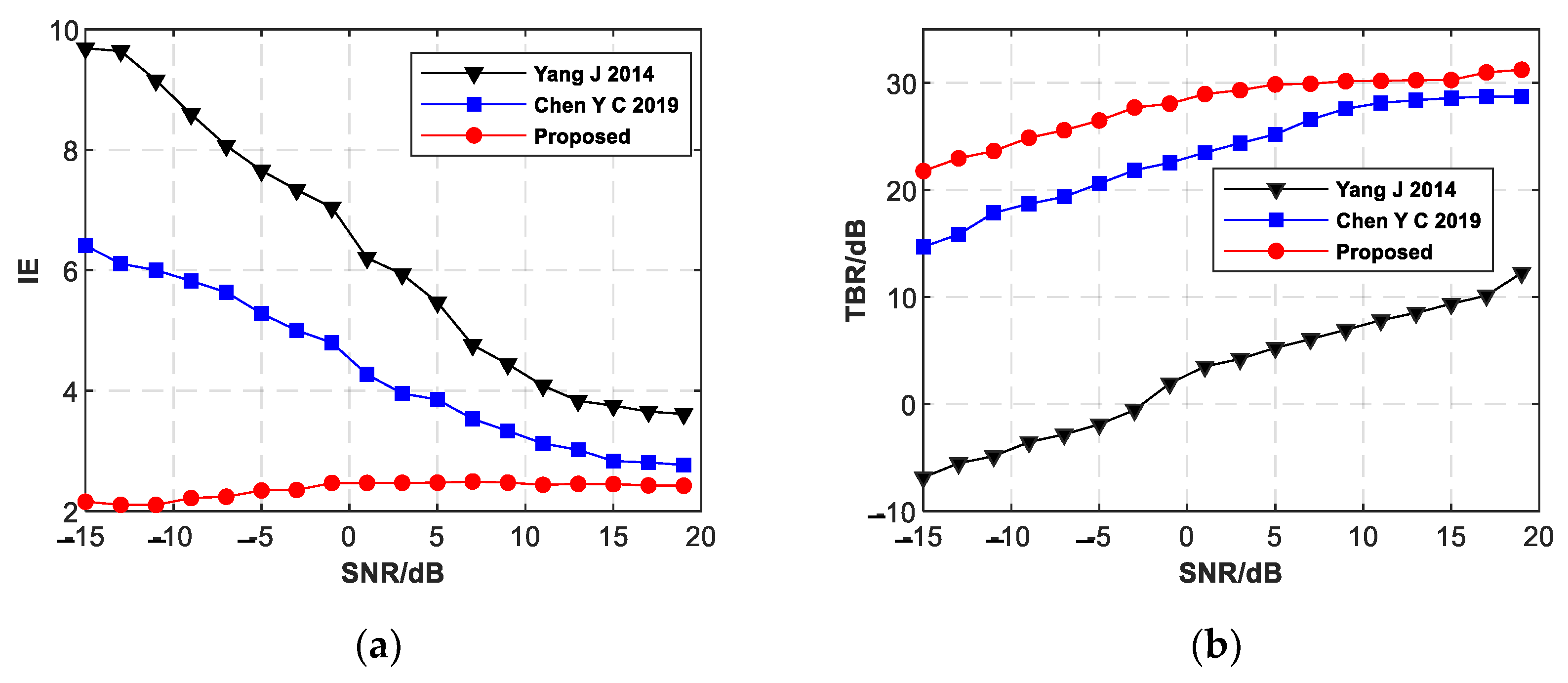
4.1.2. Comparison of Different SNRs

To test the robustness of the proposed method to noise, we added −15 dB to 20 dB of Gaussian white noise to the test echo signal in 2 dB steps. In the meantime, the echo signal was randomly down sampled with η = 0.5 . The imaging results of the three methods are given in Figure 6 for SNRs with −15 dB, 0 dB, and 15 dB, respectively. It can be seen that in the method in [8], the moving target was completely drowned in noise, and the method in [17] also failed to obtain clear results due to noise interference, whereas the proposed method achieved clearer focused SAR images of the moving target under low SNR.
The imaging performance curves for different evaluation metrics versus SNR are given in Figure 7. As can be seen from Figure 7, the imaging performance of the method in [8,17] deteriorated sharply (IE, TBR) as the SNR decreased. On the contrary, the IE of the proposed method remained basically unchanged, and the TBR in the proposed method, although showing a downward trend as SNR decreased, was generally better than the other two algorithms, which indicates the robustness of GMTSI-Net. Overall, the performance of the proposed method in terms of TBR, IE, and other related evaluation indicators was superior to the other two methods at the same SNR. Performance curves in Figure 7 demonstrate the effectiveness and robustness of the proposed method.
.

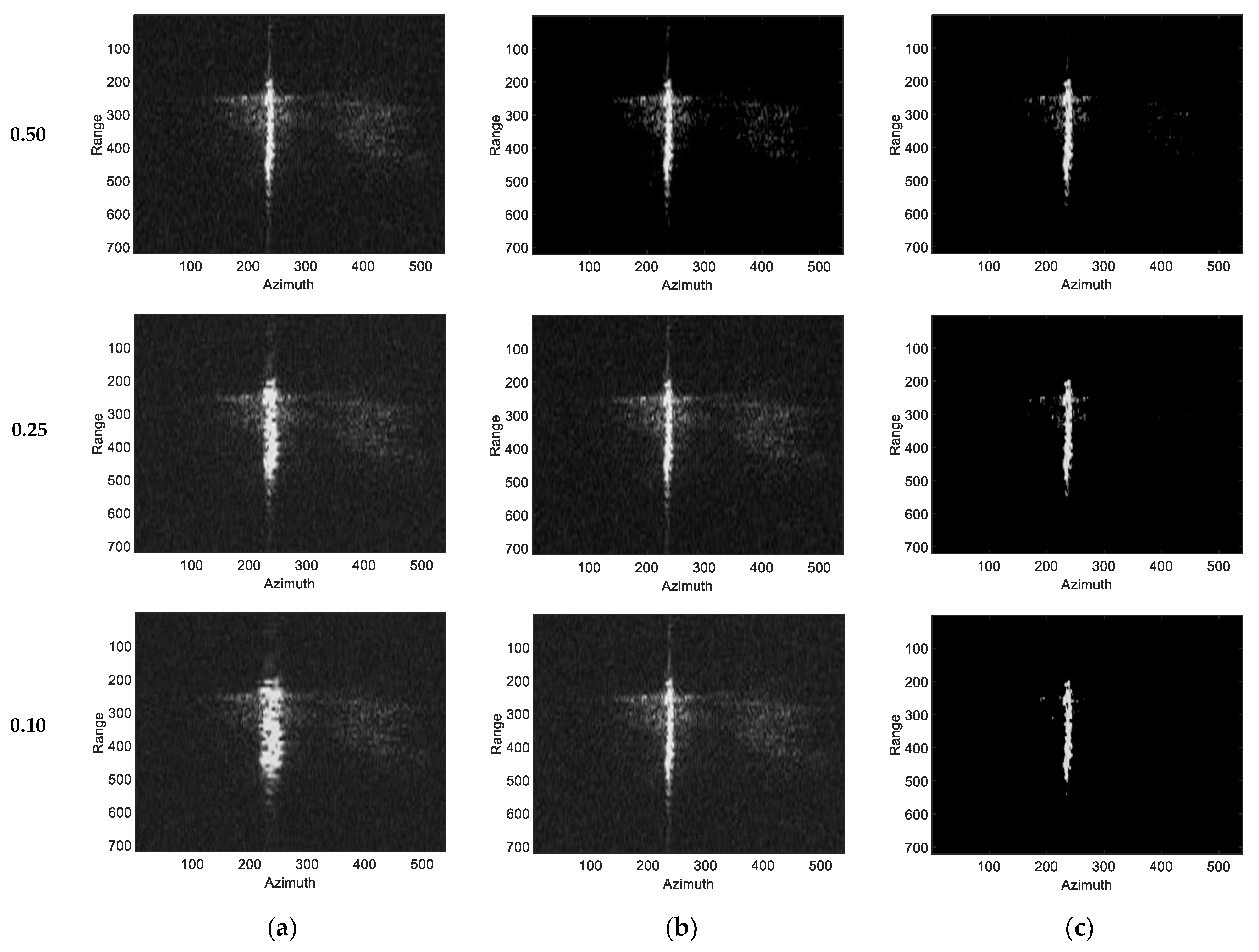
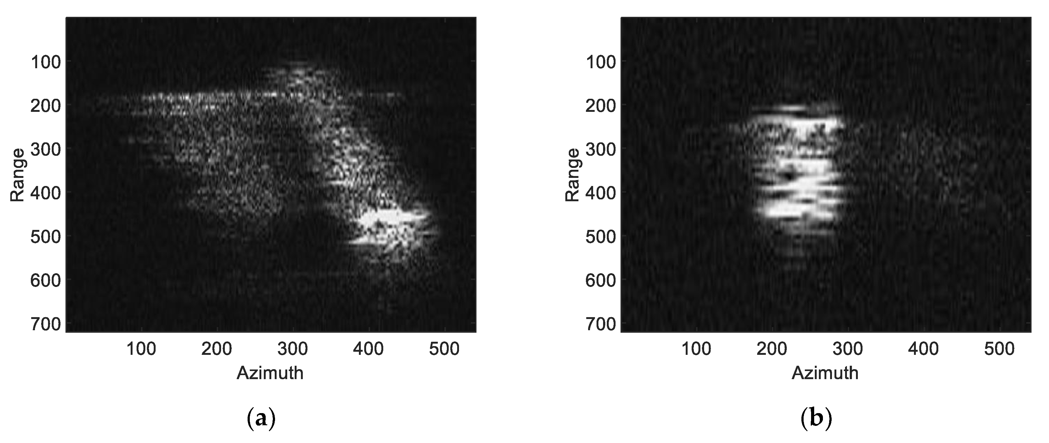
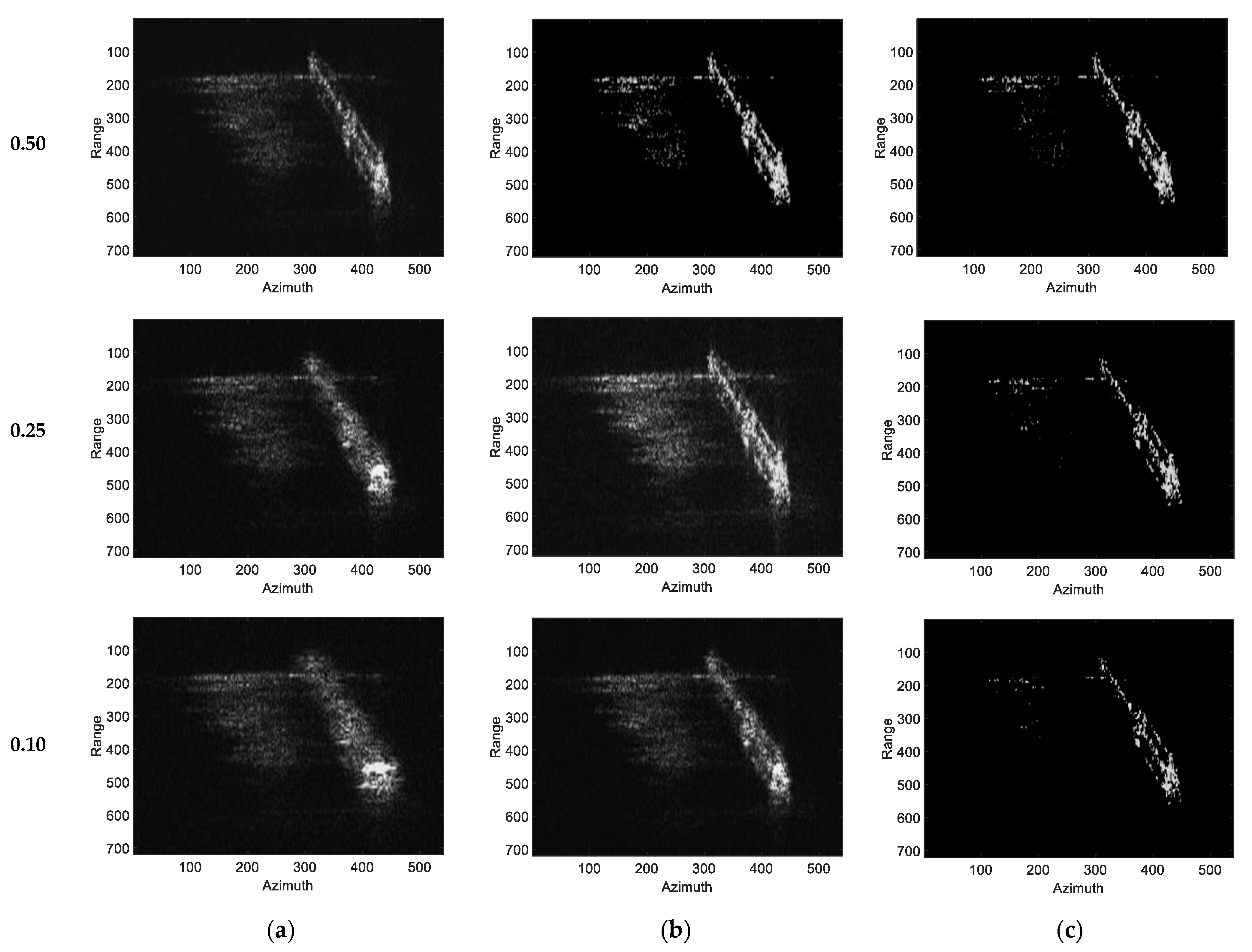
4.2. Measured Data Experiment

We further verified the imaging performance of the proposed method using the measured data of the Gaofen-3 satellite (GF-3), which is a remote sensing satellite of China’s Gaofen Special Project. It is a radar remote sensing satellite with a resolution of 1 m. The corresponding radar parameters were set as follows: The operating carrier frequency was 10 GHz, the bandwidth was 150 MHz, the pulse repetition frequency was 2500 Hz, and the distance from the center of the scene was 10,000 m. Due to the lack of enough SAR moving target datasets in terms of training, we used the SAR Ship Detection Dataset (SSDD) [36] as the training set. The two-dimensional velocity distribution of the ship target in SSDD was set as v x ( 0 , 15 ] , v y ( 0 , 20 ] .
In the testing stage, the measured data of GF-3 was used as the test set. Figure 8 shows the result of imaging the measured data of GF-3 using the stationary target RD imaging algorithm. It can be seen that the ship was out of focus due to the motion.
To obtain the focused SAR images of moving targets, we used the method in [8,17], and the proposed method to image two types of ship targets. The experimental conditions were the same as in Section 4.1.1. The imaging results are shown in Figure 9 and Figure 10. From a longitudinal comparison of Figure 9 and Figure 10, as the sampling ratio decreased, the imaging quality of the method in [8,17] gradually decreased. On the contrary, the proposed method could still image moving ship targets with a low sampling ratio. From the horizontal comparison, all three methods could focus accurately on moving targets at high sampling ratios, but the proposed method was more effective in suppressing interference from the side lobe and had better image quality. Besides, Table 2 gives the values of the relevant evaluation indicators for the measured data experiments. It should be noted that evaluation indicators such as MSE, PSNR, and TBR did not apply to this experiment due to the lack of corresponding labels. It can be seen that for two types of ship targets and different sampling ratios, the GMTSI-Net outperformed the method in [8,17] on IE to a great extent. In addition, after the learnable parameters in the proposed method are fixed by supervised training, a simple matrix multiplication operation is all that is required to obtain a focused SAR image of the moving target, which significantly reduces the time required for imaging.

5. Conclusions

In this paper, a SAR-GMT sparse imaging network, GMTSI-Net, is proposed that can effectively improve the imaging quality and computational efficiency under the condition of a low sampling ratio or SNR. Firstly, based on the derivation of the echo signal model of SAR-GMT, the imaging algorithm under the condition of known Doppler or 2-D velocity parameters was deduced. Then, based on the sparsity of SAR-GMT echo signal, a 2-D sparse observation model based on the matched filter operator was established, and the solution process of the observation model was mapped to each layer of the neural network and the unknown parameters such as the Doppler center and tuning frequency were set to learnable network parameters. Through supervised training, the GMTSI-Net could obtain imaging parameters with better imaging quality. Furthermore, we added an adaptive unfolding module to improve the flexibility of the GMTSI-Net while ensuring image quality. At the same time, two regularization constraints μ 1 Ξ ^ i 1 and μ 2 Ξ ^ i 2 2 were added to the training loss function to further ensure the quality and sparsity of the imaging results without affecting the parameter convergence. Finally, based on the simulated and GF-3 measured data, we conducted experiments and comparisons under different sampling ratios (as low as 0.1) and SNRs (as bad as −15 dB) conditions to verify the effectiveness and reliability of the proposed method.
It should be noted that, however, the proposed method failed to solve the imaging problem of multiple moving objects. This is because when imaging multiple targets, the Doppler parameters or the velocities of each moving target are different. It is not possible to focus imaging on multiple moving targets with GMTSI-Net alone. Therefore, how to accurately estimate the Doppler parameters of each moving target in the network and achieve the focusing result of multiple moving targets will be the focus of our future research work.

Author Contributions

Conceptualization and methodology, L.C. and J.N.; software, L.C. and J.N.; validation, L.C., X.L. and J.N.; resources, J.N. and Y.L.; writing—review and editing, L.C., J.N., Y.L. and Q.H.; funding acquisition, Y.L. and J.N. All authors have read and agreed to the published version of the manuscript.

Funding

This research was funded by the National Natural Science Foundation of China under grants 62001508 and 62131020.

Data Availability Statement

Not applicable.

Conflicts of Interest

The authors declare no conflict of interest.

Appendix A

For the convenience of derivation, we ignored the constant term in Equation (26), and represented the matrix in it as a vector:
L o s s ( ϒ ) = vec ( Ξ ^ i Ξ label 2 2 ) + vec ( μ 1 Ξ ^ i 1 ) vec ( μ 2 Ξ ^ i 2 2 )
The first term in (A1) can be expanded as:
vec ( Ξ ^ i Ξ label 2 2 ) = vec ( ( Ξ ^ i ) H Ξ ^ i + ( Ξ label ) H Ξ label ( Ξ ^ i ) H Ξ label ( Ξ label ) H Ξ ^ i )
where H is the conjugate operation of the matrix. Then, the gradient of (A2) can be expressed as:
vec ( Ξ ^ i Ξ label 2 2 ) = vec [ 2 ( Ξ ^ i Ξ label ) ]
Then, we calculated the gradient of the second and last terms in Equation (26). Take the second item as an example. Since the second term is the L1 norm, it can be approximated as:
vec ( Ξ ^ i 1 ) = vec ( ( Ξ ^ i ) H Ξ ^ i + ζ )
where ζ is a small smoothing parameter. Based on the above formula, we can get the gradient of the second term as:
vec ( Ξ ^ i 1 ) = vec ( D 1 Ξ ^ i )
where D 1 is a diagonal matrix, which can be specifically expressed as:
d i = | Ξ ^ i | 2 + ζ
We can also get the gradient of the last term in Equation (26) as follows:
vec ( Ξ ^ i 2 2 ) = vec ( Ξ ^ i )
Hence, the gradient of the loss function can be written as:
L o s s ( ϒ ) = vec [ 2 ( Ξ ^ i Ξ label ) μ 2 Ξ ^ i + μ 1 D 1 Ξ ^ i ] = vec [ ( 2 μ 2 ) Ξ ^ i + μ 1 D 1 Ξ ^ i 2 Ξ label ]

References

  1. Zhou, F.; Zhao, B.; Tao, M.; Bai, X.; Chen, B.; Sun, G. A large scene deceptive jamming method for space-borne SAR. IEEE Trans. Geosci. Remote Sens. 2013, 51, 4486–4495. [Google Scholar] [CrossRef]
  2. Perry, R.P.; Di Pietro, R.C.; Fante, R. SAR Imaging of Moving Targets. IEEE Trans. Aerosp. Electron. Syst. 1999, 35, 188–200. [Google Scholar] [CrossRef]
  3. Jen, K.J. Theory of synthetic aperture radar imaging of a moving target. IEEE Trans. Geosci. Remote Sens. 2001, 39, 1984–1992. [Google Scholar]
  4. Fienup, J.R. Detecting moving targets in SAR imagery by focusing. IEEE Trans. Aerosp. Electron. Syst. 2001, 37, 794–809. [Google Scholar] [CrossRef]
  5. Tong, X.; Bao, M.; Sun, G.; Han, L.; Zhang, Y.; Xing, M. Refocusing of Moving Ships in Squint SAR Images Based on Spectrum Orthogonalization. Remote Sens. 2021, 13, 2807. [Google Scholar] [CrossRef]
  6. He, Z.; Chen, X.; Yi, T.; He, F.; Dong, Z.; Zhang, Y. Moving Target Shadow Analysis and Detection for ViSAR Imagery. Remote Sens. 2021, 13, 3012. [Google Scholar] [CrossRef]
  7. Zhou, F.; Wu, R.; Xing, M.; Bao, Z. Approach for single channel SAR ground moving target imaging and motion parameter estimation. IET Radar Sonar Navig. 2007, 1, 59–66. [Google Scholar] [CrossRef]
  8. Yang, J.; Liu, C.; Wang, Y. Imaging and Parameter Estimation of Fast-Moving Targets with Single-Antenna SAR. IEEE Geosci. Remote Sens. Lett. 2014, 11, 529–533. [Google Scholar] [CrossRef]
  9. Li, G.; Xia, X.; Peng, Y. Doppler Keystone Transform: An Approach Suitable for Parallel Implementation of SAR Moving Target Imaging. IEEE Geosci. Remote Sens. Lett. 2008, 5, 573–577. [Google Scholar] [CrossRef]
  10. Wan, J.; Tan, X.; Chen, Z.; Li, D.; Liu, Q.; Zhou, Y.; Zhang, L. Refocusing of Ground Moving Targets with Doppler Ambiguity Using Keystone Transform and Modified Second-Order Keystone Transform for Synthetic Aperture Radar. Remote Sens. 2021, 13, 177. [Google Scholar] [CrossRef]
  11. Chen, V.C.; Lipps, R.; Bottoms, M. FOPEN SAR imaging of ground moving targets using rotational time-frequency-Radon transforms. In Proceedings of the 2002 IEEE Radar Conference, Long Beach, CA, USA, 25 April 2002; pp. 154–159. [Google Scholar]
  12. Huang, P.H.; Xia, X.G.; Gao, Y.S.; Liu, X.Z.; Liao, G.S.; Jiang, X. Ground Moving Target Refocusing in SAR Imagery Based on RFRT-FrFT. IEEE Trans.Geosci. Remote Sens. 2019, 57, 5476–5492. [Google Scholar] [CrossRef]
  13. Leibovich, M.; Papanicolaou, G.; Tsogka, C. Low Rank Plus Sparse Decomposition of Synthetic Aperture Radar Data for Target Imaging. IEEE Trans. Comput. Imaging 2020, 6, 491–502. [Google Scholar] [CrossRef]
  14. Kang, M.S.; Kim, K.T. Ground Moving Target Imaging Based on Compressive Sensing Framework with Single-Channel SAR. IEEE Sens. J. 2020, 20, 1238–1250. [Google Scholar] [CrossRef]
  15. Gu, F.F.; Zhang, Q.; Chen, Y.C.; Huo, W.J.; Ni, J.C. Parametric sparse representation method for motion parameter estimation of ground moving target. IEEE Sens. J. 2016, 16, 7646–7652. [Google Scholar] [CrossRef]
  16. Chen, Y.; Li, G.; Zhang, Q.; Sun, J. Refocusing of Moving Targets in SAR Images via Parametric Sparse Representation. Remote Sens. 2017, 9, 795. [Google Scholar] [CrossRef]
  17. Chen, Y.C.; Li, G.; Zhang, Q. Iterative Minimum Entropy Algorithm for Refocusing of Moving Targets in SAR Images. IET Radar Sonar Navig. 2019, 13, 1279–1286. [Google Scholar] [CrossRef]
  18. Bu, H.X.; Bai, X.; Tao, R. Compressed sensing SAR imaging based on sparse representation in fractional Fourier domain. Sci. China Inf. Sci. 2012, 55, 1789–1800. [Google Scholar] [CrossRef]
  19. Wu, D.; Yaghoobi, M.; Davies, M.E. Sparsity-driven GMTI processing framework with multichannel SAR. IEEE Trans. Geosci. Remote Sens. 2019, 57, 1434–1447. [Google Scholar] [CrossRef]
  20. Kelly, S.; Yaghoobi, M.; Davies, M.E. Sparsity-based autofocus for undersampled synthetic aperture radar. IEEE Trans. Aerosp. Electron. Syst. 2014, 50, 972–986. [Google Scholar] [CrossRef]
  21. Geng, J.; Yu, Z.; Li, C.; Liu, W. Squint Mode GEO SAR Imaging Using Bulk Range Walk Correction on Received Signals. Remote Sens. 2019, 11, 17. [Google Scholar] [CrossRef]
  22. Zhang, X.P.; Liao, G.; Zhu, S.Q.; Yang, D.; Du, W.T. Efficient Compressed Sensing Method for Moving-Target Imaging by Exploiting the Geometry Information of the Defocused Results. IEEE Geosci. Remote Sens. Lett. 2015, 12, 517–521. [Google Scholar] [CrossRef]
  23. Li, J.; Xu, C.; Su, H.; Gao, L.; Wang, T. Deep Learning for SAR Ship Detection: Past, Present and Future. Remote Sens. 2022, 14, 2712. [Google Scholar] [CrossRef]
  24. Zhao, S.Y.; Zhang, Z.H.; Zhang, T.; Guo, W.W.; Luo, Y. Transferable SAR Image Classification Crossing Different Satellites Under Open Set Condition. IEEE Geosci. Remote Sens. Lett. 2022, 19, 1–5. [Google Scholar] [CrossRef]
  25. Yang, M.J.; Bai, X.R.; Wang, L.; Zhou, F. Mixed Loss Graph Attention Network for Few-Shot SAR Target Classification. IEEE Trans. Geosci. Remote Sens. 2022, 60, 5216613. [Google Scholar] [CrossRef]
  26. Bai, X.R.; Zhang, Y.J.; Liu, S.Q. High-Resolution Radar Imaging of Off-Grid Maneuvering Targets Based on Parametric Sparse Bayesian Learning. IEEE Trans. Geosci. Remote Sens. 2022, 60, 1–11. [Google Scholar] [CrossRef]
  27. Mu, H.L.; Zhang, Y.; Ding, C.; Jiang, Y.C. DeepImaging: A Ground Moving Target Imaging Based on CNN for SAR-GMTI System. IEEE Geosci. Remote Sens. Lett. 2021, 18, 117–121. [Google Scholar] [CrossRef]
  28. Lu, Z.J.; Qin, Q.; Shi, H.Y.; Huang, H. SAR moving target imaging based on convolutional neural network. Digit. Signal Process. 2020, 106, 102832. [Google Scholar] [CrossRef]
  29. Ito, D.; Takabe, S.; Wadayama, T. Trainable ISTA for Sparse Signal Recovery. IEEE Trans. Signal Process. 2019, 67, 3113–3125. [Google Scholar] [CrossRef]
  30. Zhang, J.; Ghanem, B. ISTA-Net: Interpretable Optimization-Inspired Deep Network for Image Compressive Sensing. In Proceedings of the IEEE Conference on Computer Vision and Pattern Recognition, Salt Lake City, UT, USA, 18–22 June 2018; pp. 1828–1837. [Google Scholar]
  31. Yonel, B.; Mason, E.; Yazıcı, B. Deep learning for passive synthetic aperture radar. IEEE J. Sel. Top. Signal Process. 2018, 12, 90–103. [Google Scholar] [CrossRef]
  32. Wei, S.J.; Liang, J.D.; Wang, M.; Shi, J.; Zhang, X.L.; Ren, H.R. AF-AMPNet: A Deep Learning Approach for Sparse Aperture ISAR Imaging and Autofocusing. IEEE Trans. Geosci. Remote Sens. 2022, 60, 5206514. [Google Scholar] [CrossRef]
  33. Zhao, S.Y.; Ni, J.C.; Liang, J.; Xiong, S.C.; Luo, Y. End-to-End SAR Deep Learning Imaging Method Based on Sparse Optimization. Remote Sens. 2021, 13, 4429. [Google Scholar] [CrossRef]
  34. Vujović, S.; Stanković, I.; Daković, M.; Stanković, L. Comparison of a gradient-based and LASSO (ISTA) algorithm for sparse signal reconstruction. In Proceedings of the 2016 5th Mediterranean Conference on Embedded Computing (MECO), Bar, Montenegro, 12–16 June 2016; pp. 377–380. [Google Scholar]
  35. Zou, F.Y.; Shen, L.; Jie, Z.Q.; Zhang, W.Z.; Liu, W. A Sufficient Condition for Convergences of Adam and RMSProp. In Proceedings of the IEEE/CVF Conference on Computer Vision and Pattern Recognition (CVPR), Long Beach, CA, USA, 15–20 June 2019; pp. 11119–11127. [Google Scholar]
  36. Zhang, T.; Zhang, X.; Li, J.; Xu, X.; Wang, B.; Zhan, X.; Xu, Y.; Ke, X.; Zeng, T.; Su, H. SAR Ship Detection Dataset (SSDD): Official Release and Comprehensive Data Analysis. Remote Sens. 2021, 13, 3690. [Google Scholar] [CrossRef]
Figure 1. The geometry of the side-looking SAR platform and a ground-moving target.
Remotesensing 14 04404 g001
Figure 2. Flow chart of SAR-GMT imaging algorithm.
Remotesensing 14 04404 g002
Figure 3. The architecture of GMTSI-Net.
Remotesensing 14 04404 g003
Figure 4. Schematic diagram of a tank model.
Remotesensing 14 04404 g004
Figure 5. Imaging results of three methods with different sampling ratios. (a) SAR-GMT echo signals with different sampling ratios; (b) Imaging results of the method in [8]; (c) Imaging results of the method in [17]; (d) Imaging results of the proposed method.
Remotesensing 14 04404 g005
Figure 6. Imaging results of three methods with different SNRs. (a) Imaging results of the method in [8]; (b) Imaging results of the method in [17]; (c) Imaging results of the proposed method.
Remotesensing 14 04404 g006
Figure 7. Performance curves of (a) ENT. (b)TBR versus SNR of three methods with sampling ratio η = 0.5 .
Remotesensing 14 04404 g007
Figure 8. Imaging result of two ship targets from GF-3 measured data with traditional RDA. (a) Ship 1; (b) ship 2.
Remotesensing 14 04404 g008
Figure 9. Imaging result of ship 1 from GF-3 measured data with different methods. (a) Imaging results of the method in [8]; (b) Imaging results of the method in [17]; (c) Imaging results of the proposed method.
Remotesensing 14 04404 g009
Figure 10. Imaging result of ship 2 from GF-3 measured data with different methods. (a) Imaging results of the method in [8]; (b) Imaging results of the method in [17]; (c) Imaging results of the proposed method.
Remotesensing 14 04404 g010
Table 1. Evaluation of different sampling ratios.
Sampling
Ratio
MethodMSEPSNRIETBRImaging
Time (s)
0.50Method in [8]558.0720.664.08799.366.581
Method in [17]60.7530.292.830928.58138.52
Proposed50.7331.082.422130.260.924
0.25Method in [8]967.1818.275.69643.724.865
Method in [17]113.6927.574.000620.7698.25
Proposed74.0829.432.359828.310.641
0.10Method in [8]2672.7313.866.9410−5.633.021
Method in [17]330.7523.944.656915.3850.86
Proposed109.6127.732.215029.050.402
Table 2. Evaluation of measured experiments.
TargetSampling RatioMethodIEImaging Time (s)
Ship 10.50Method in [8]4.660012.081
Method in [17]2.5668407.526
Proposed2.16031.453
0.25Method in [8]4.99439.574
Method in [17]3.1532295.186
Proposed1.88230.973
0.10Method in [8]5.57295.158
Method in [17]3.8129209.26
Proposed1.54930.843
Ship 20.50Method in [8]4.452010.835
Method in [17]2.6330296.37
Proposed1.42461.102
0.25Method in [8]4.53236.421
Method in [17]2.8376173.15
Proposed1.37020.932
0.10Method in [8]4.62314.113
Method in [17]3.526896.64
Proposed1.33250.762
Publisher’s Note: MDPI stays neutral with regard to jurisdictional claims in published maps and institutional affiliations.

