1. Introduction
Synthetic aperture radar (SAR) is a high-resolution coherent imaging radar. As an active microwave remote sensing system, which is not affected by light and climatic conditions, SAR can achieve all-weather day-and-night earth detection [
1]. At the same time, SAR adopts synthetic aperture technology and matched filtering technology, which can realize long-distance high-resolution imaging. Therefore, SAR is of great significance in both military and civilian fields [
2].
In recent years, with the development of SAR technology, the ability to obtain SAR data has been greatly improved. The early methods of manually interpreting SAR images cannot support the rapid processing of large amounts of SAR data due to their low time efficiency and high cost. How to quickly mine useful information from massive high-resolution SAR image data and apply it to military reconnaissance, agricultural and forestry monitoring, geological survey and many other fields has become an important problem in SAR applications that needs to be solved urgently. Therefore, the automatic target recognition (ATR) [
3] of SAR images to solve this problem has become a research hotspot.
Since a SAR image shows the scattering characteristics of the target to electromagnetic waves, the SAR image is very different from the optical image, which also has a great impact on the SAR ATR. Classical SAR ATR methods include a template-based method and model-based method. The template-based method is one of the earliest proposed methods, including direct template matching methods that calculate the similarity between the template formed by processing the training sample itself and the test sample for classification [
4], and feature template matching methods that use classifiers such as SVM [
5], KNN [
6] and Bayes classifier [
7] after extracting various features [
8,
9] for classification. The template-based method is simple in principle and easy to implement, but requires large and diverse training data to build a complete template library. To make up for the shortcomings of the template-based method, the model-based method [
10] is proposed, which includes two parts: model construction and online prediction.
With the development of machine learning and deep learning technology, the automatic feature extraction ability of a neural network has attracted the attention of researchers, and then deep learning has been applied in SAR ATR. Initially, the neural network model in traditional computer vision (CV) was directly applied to SAR target recognition. For instance, Kang et al. transferred existing pretrained networks after fine-tuning [
11]. Unsupervised learning methods such as autoencoder [
12] and deep belief network (DBN) [
13] were also used to automatically learn SAR image features. Afterward, the network structure and loss function were designed for the specific task of target recognition using the amplitude information of SAR images, which were more in line with the requirements of the SAR target recognition task and undoubtedly achieved better recognition performance. Chen et al. designed a fully convolutional network (A-ConvNets) for recognition on the MSTAR target dataset [
14]. Lin et al. proposed the deep convolutional Highway Unit for ATR of a small number of SAR targets [
15]. Du et al. recommended the application of multi-task learning to SAR ATR to learn and share useful information from two auxiliary tasks designed to improve the performance of recognition tasks [
16]. Gao et al. proposed to extract polarization features and spatial features, respectively, based on a dual-branch deep convolution neural network (Dual-CNN) [
17]. Shang et al. designed deep memory convolution neural networks (M-Net), including an information recorder to remember and store samples’ spatial features [
18]. Recently, the characteristics brought by the special imaging mechanism of SAR are being focused on, and some methods combining deep learning with physical models have appeared. Zhang et al. proposed a domain knowledge-powered two-stream deep network (DKTS-N), which incorporates a deep learning network with SAR domain knowledge [
19]. Feng et al. combined electromagnetic scattering characteristics with a depth neural network to introduce a novel method for SAR target classification based on an integration parts model and deep learning algorithm [
20]. Wang et al. recommended an attribute-guided multi-scale prototypical network (AG-MsPN) that obtains more complete descriptions of targets by subband decomposition of complex-valued SAR images [
21]. Zhao et al. proposed a contrastive-regulated CNN in the complex domain to obtain a physically interpretable deep learning model [
22]. Compared with traditional methods, deep learning methods have achieved better recognition results in SAR ATR. However, most of these current SAR ATR methods based on deep learning are aimed at single-aspect SAR images.
In practical applications, due to the special imaging principle of SAR, the same target will show different visual characteristics under different observation conditions, which also makes the performance of SAR ATR methods affected by various factors, such as environment, target characteristics and imaging parameters. The observation azimuth is also one of the influencing factors. The sensitivity of the scattering characteristics of artificial targets to the observation azimuth leads to a large difference in the visual characteristics of the same target at different aspects. Therefore, the single-aspect SAR image loses the scattering information related to the observation azimuth [
23]. The target recognition performance of single-aspect SAR is also affected by the aspect.
With the development of SAR systems, multi-aspect SAR technologies such as Circular SAR (CSAR) [
24] can realize continuous observation of the same target from different observation azimuth angles. The images of the same target under different observation azimuth angles obtained by multi-angle SAR contain a lot of identification information. The multi-aspect SAR target recognition technology uses multiple images of the target obtained from different aspects and combines the scattering characteristics of different aspects to identify the target category. Compared with single-aspect SAR images, multi-aspect SAR image sequences contain spatially varying scattering features [
25] and provide more identification information for the same target under different aspects. On the other hand, multi-aspect SAR target recognition can improve the target recognition performance by fully mining the intrinsic correlation between multi-aspect SAR images.
The neural networks that use multi-aspect SAR image sequences for target recognition mainly include recurrent neural networks (RNN) and convolutional neural networks (CNN). Zhang et al. proposed multi-aspect-aware bidirectional LSTM (MA-BLSTM) [
26], which extracts features from each multi-aspect SAR image through a Gabor filter, and further uses LSTM to store the sequence features in the memory unit and transmit through learnable gates. Similarly, Bai et al. proposed a bidirectional convolutional-recurrent network (BCRN) [
27], which uses Deep CNN to replace the manual feature extraction process of MA-BLSTM. Pei et al. proposed a multiview deep convolutional neural network (MVDCNN) [
28], which uses a parallel CNN to extract the features of each multi-aspect SAR image, and then merges them one by one through pooling. Based on MVDCNN, Pei et al. improved the original network with the convolutional gated recurrent unit (ConvGRU) and proposed a multiview deep feature learning network (MVDFLN) [
29].
Although these methods have obtained good recognition results, there are still the following problems:
When using RNN or CNN to learn the association between multi-aspect SAR images, the farther the two images are in a multi-aspect SAR image sequence, the more difficult it is to learn the association between them. That is, the association will depend on the order of the image in the sequence.
All current studies require a lot of data for training the deep networks, and the accuracy will drop sharply in the case of few samples.
The existing approaches do not consider the influence of noise, which leads to a poor anti-noise ability of the model.
To address these problems, in this paper, we propose a multi-aspect SAR target recognition method based on convolutional autoencoder (CAE) and self-attention. After pre-training, the encoder of CAE will be used to extract the features of single-aspect SAR images in the multi-aspect SAR image sequence, and then the intrinsic correlation between images in the sequence will be mined through a transformer based on self-attention.
In this paper, it is innovatively proposed to mine the correlation between multi-aspect SAR images through a transformer [
30] based on self-attention. Vision transformer (ViT) [
31] for optical image classification and the networks based on attention for single-aspect SAR ATR, such as the mixed loss graph attention network (MGA-Net) [
32] and the convolutional transformer (ConvT) [
33], extract representative features by determining the correlation between various parts of an image itself. Unlike them, the ideas of natural language processing (NLP) tasks are leveraged to mine the association between the semantic information of each image in the multi-aspect SAR image sequence. Because each image is correlated with other images in the same way in the calculation process of self-attention, the order dependence problem faced by existing methods will be avoided. Considering that self-attention loses local details, the CNN pre-trained by CAE with shared parameters is designed to extract local features for each image in the sequence. On the one hand, effective feature extraction provided by CNN can diminish the requirement for sample size. On the other hand, by minimizing the gap between the reconstructed image and the original input, the autoencoder ensures that the features extracted by the encoder can effectively represent the principal information of the original image. Thus CAE plays a vital role in anti-noise.
Compared with available multi-aspect SAR target recognition methods, the novelty as well as the contribution of the proposed method can be summarized as follows.
A multi-aspect SAR target recognition method based on self-attention is proposed. Compared with existing methods, the calculation process of self-attention makes it not affected by the order of images in the sequence. To the best of our knowledge, this is the first attempt to apply a transformer based on self-attention to complete the recognition task of multi-aspect SAR image sequences.
CAE is introduced for feature extraction in our method, which is due to the additional consideration of the cases with few samples and noise compared with other methods and is created to improve the ability of the network to effectively extract the major features through pre-training and fine-tuning.
Compared with the existing methods designed for multi-aspect SAR target recognition, our network obtains higher recognition accuracy on the MSTAR dataset and exhibits more robust recognition performance in version and configuration variants. Furthermore, our method demonstrates better in the recognition task with a small number of samples. Our method achieves stronger performance in anti-noise assessment as well.
The remainder of this paper is organized as follows:
Section 2 describes the proposed network structure in detail.
Section 3 presents the experimental details and results.
Section 4 discusses the advantages and future work of the proposed method.
Section 5 summarizes the full paper.
2. Multi-Aspect SAR Target Recognition Framework
2.1. Overall Structure
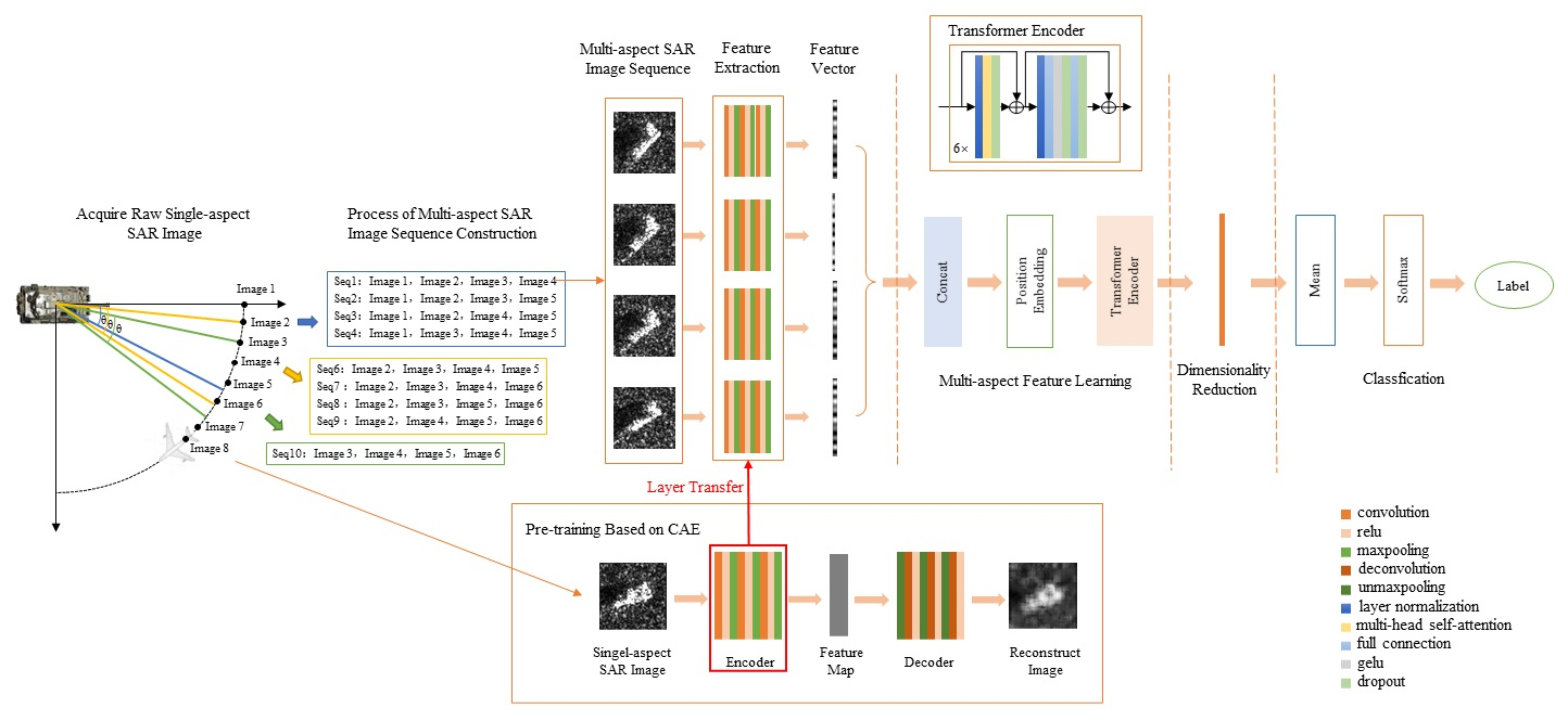
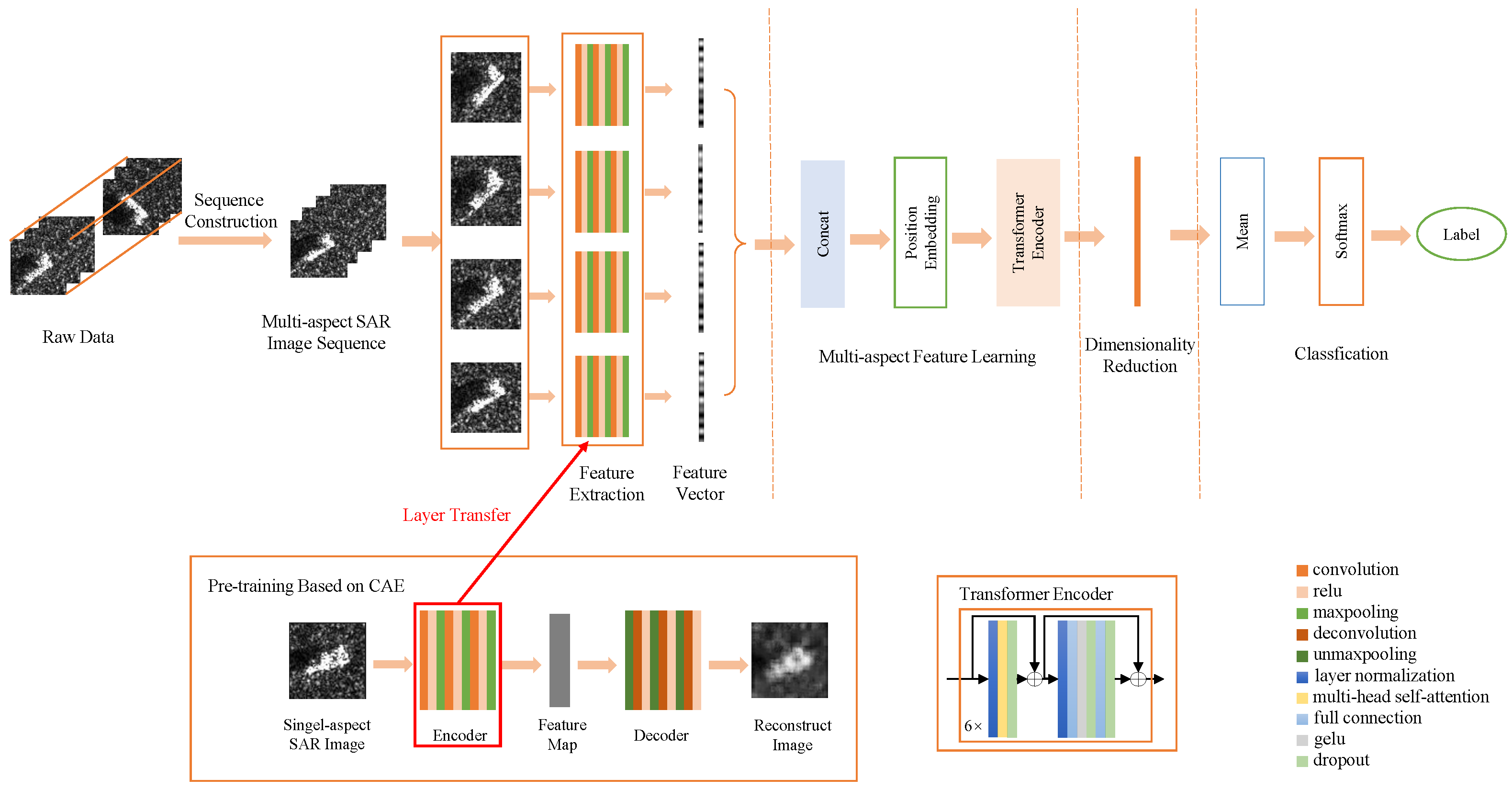
As shown in
Figure 1, the proposed multi-aspect SAR target recognition method consists of five parts, i.e., multi-aspect SAR image sequence construction, single-aspect feature extraction, multi-aspect feature learning, feature dimensionality reduction and target classification. Among them, feature extraction is implemented using CNN pretrained by CAE, and multi-aspect feature learning uses the transformer encoder [
31] structure based on self-attention.
Before feature extraction, single-aspect SAR images are used to construct multi-aspect SAR image sequences and also serve as the input to pre-train CAE, which includes the encoder that utilizes the multi-layer convolution-pooling structure to extract features and the decoder that utilizes the multi-layer deconvolution-unpooling structure to reconstruct images. The encoder of CAE after pre-training will be transferred to CNN for feature extraction of each image in the input multi-aspect SAR image sequence. In particular, the output of feature extraction for an image is a 1-D feature vector. Then, in the multi-aspect feature learning structure, the vectorized features extracted from each image are spliced and added to position embedding to be the input of the transformer encoder based on multi-head self-attention. All the output features of the transformer encoder are reduced in dimension by convolutions and then averaged. Finally, the softmax classifier gives the recognition result.
In the training process, the whole network obtains errors from the output and propagates back along the network to update parameters. It should be noted that the parameters of multi-layer CNN used for feature extraction can be frozen or updated with the entire network for fine-tuning.
In the following discussions, the details of each part of the proposed method and the training process will be introduced in turn, such as the loss function and so forth.
2.2. Multi-Aspect SAR Image Sequence Construction
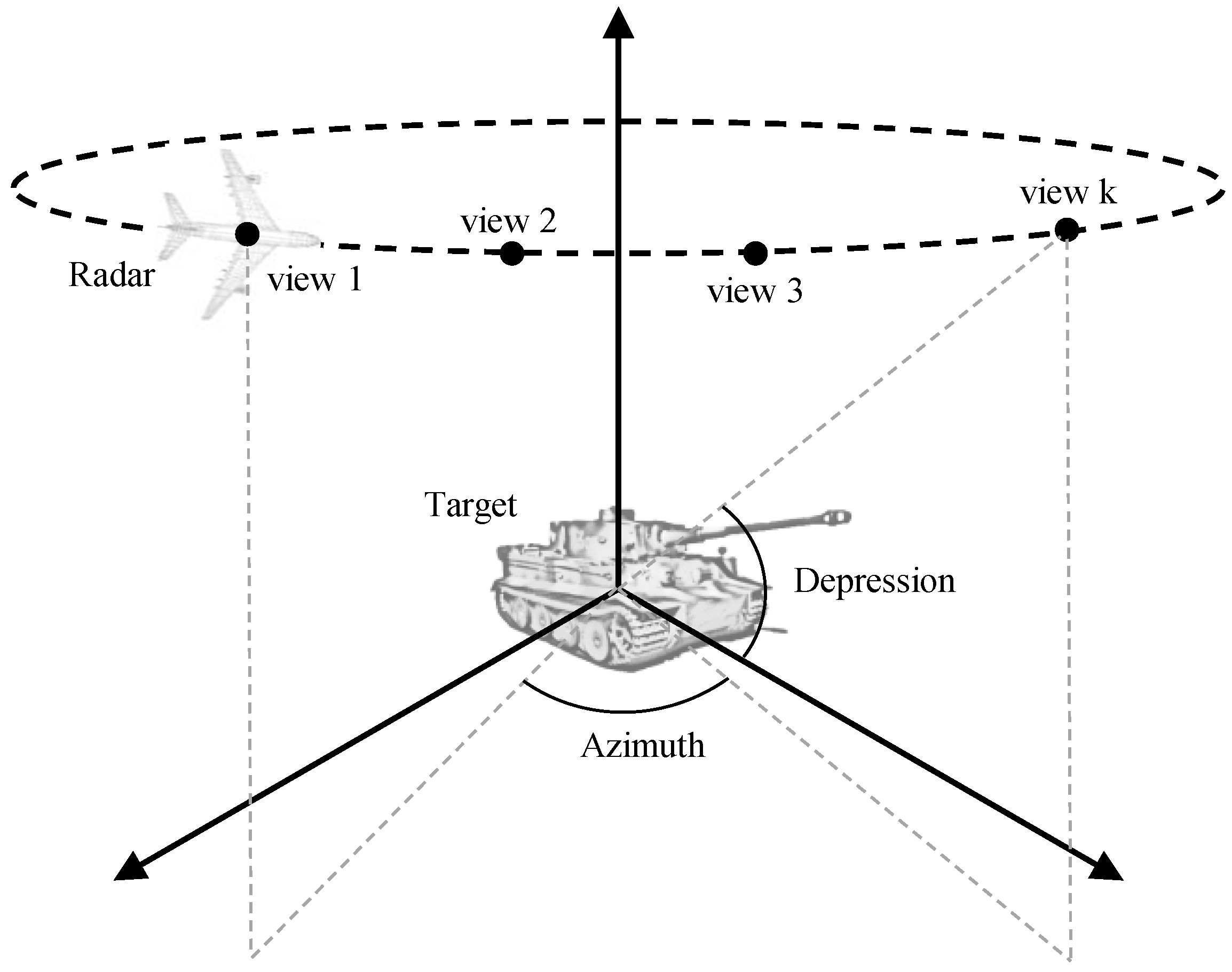
Multi-aspect SAR images can be obtained by imaging the same target from different azimuth angles and different depression angles by radars on one or more platforms.
Figure 2 shows a simple geometric model for multi-aspect SAR imaging.
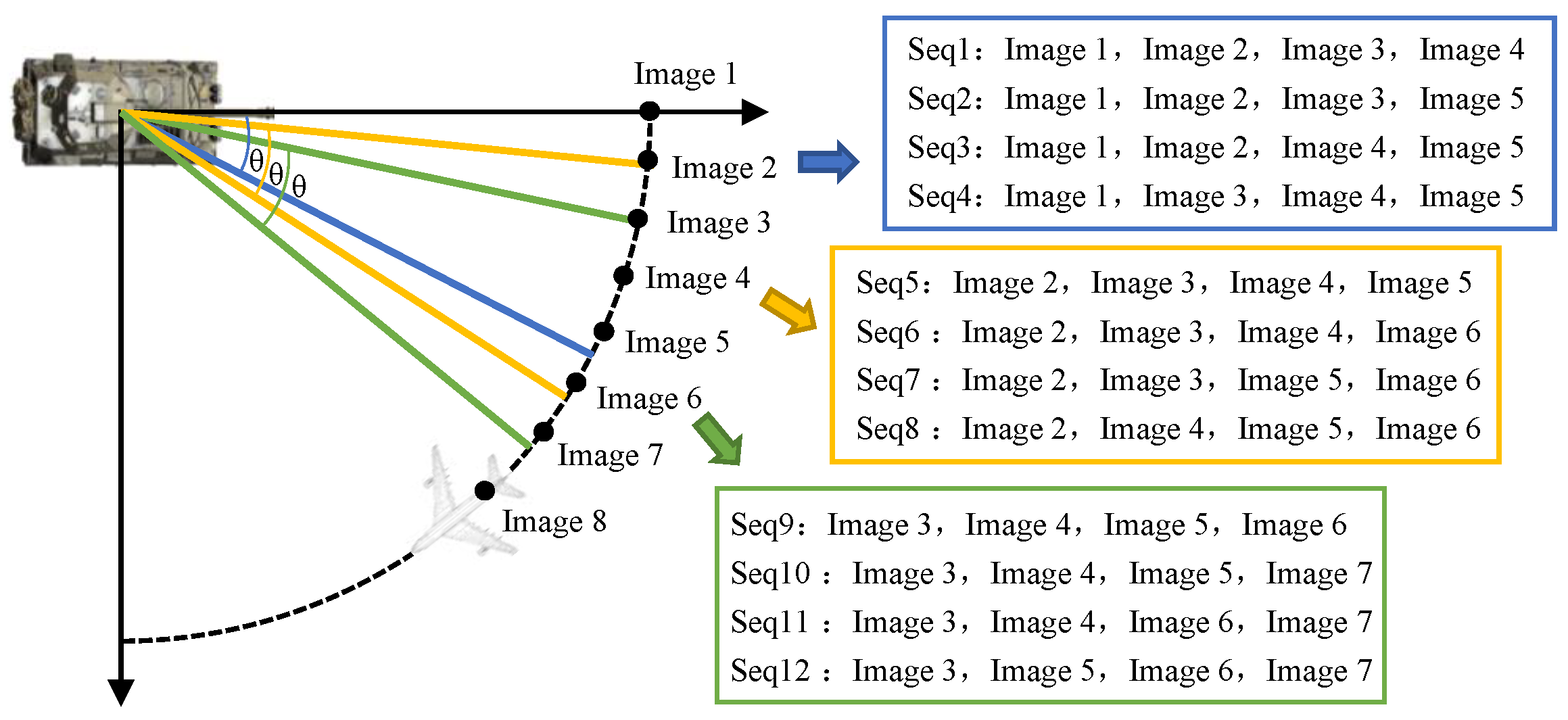
On this basis, multi-aspect SAR image sequences are built based on the following rules. Suppose is the raw SAR image set, where is the image set sorted by azimuth angle for a specific class . C is the number of classes and is the number of images contained in one class. The azimuth of the image is . For a given angle range and sequence length k, a window with fixed length is placed along the original image set with a stride of 1 and the images in the window form k sequences of length k by permutation, then the sequence whose azimuth difference between any two images is smaller than is reserved as the training sample of the network. In addition, the final retained sequence samples are required to not contain duplicate samples. The process of multi-aspect SAR image sequence construction is summarized in Algorithm 1. In Algorithm 1, is the multi-aspect SAR image sequence, where is the sequence set for a specific class . is the number of sequences contained in one class.
Figure 3 shows an example of multi-aspect SAR image sequence construction. When the sequence length is set to 4, ideally, 12 sequence samples can be received from only 7 images. In this way, enough training samples can be obtained from limited raw SAR images.
| Algorithm 1 Construct multi-aspect SAR image sequence |
Input: angle range and sequence length k, raw SAR images , and class labels Output: multi-aspect SAR image sequence for to C do for to do if Construct all possible sequence except else if Construct the sequence end for if Construct the sequence Get end for |
2.3. Feature Extraction Pre-Trained by CAE
Drawing on the idea of NLP, our method considers each image in a multi-aspect SAR image sequence to be equivalent to each word in a sentence. To effectively extract major features from each image in a multi-aspect SAR image sequence in parallel, CNN pre-trained by CAE with shared parameters is designed, which can reduce the number of learning parameters as well.
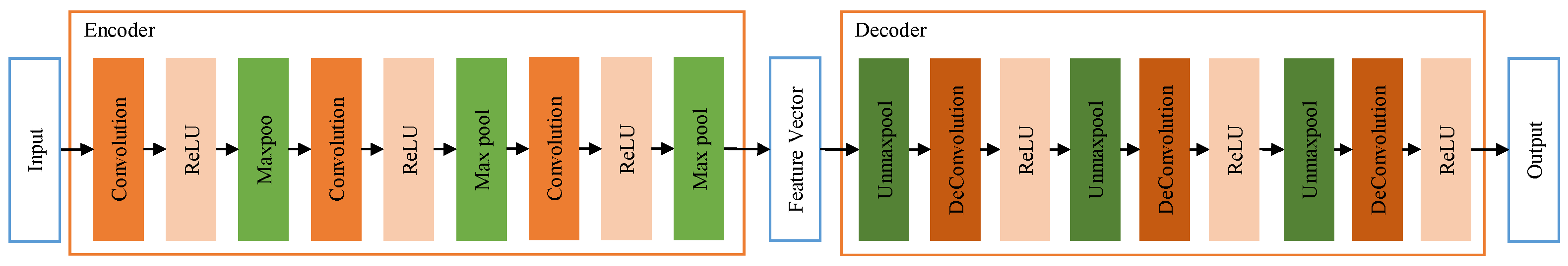
Figure 4 shows the network structure of CAE, which consists of an encoder and decoder.
The encoder is comprised of convolutional layers, pooling layers and the nonlinear activation function. The convolutional layer is the core structure, which extracts image features through convolution operations. The convolution layer in the neural network initializes a learnable convolution kernel, which is convolved with the input vector to obtain a feature map. Each convolution kernel has a bias, which is also trainable. The activation function is a mapping from the input to the output of the neural network, which increases the nonlinear properties of the neural network. ReLU, which is simple to calculate and can speed up the convergence of the network, is used as the activation function in the encoder of CAE. The convolutional layer is usually followed by the pooling layer, which plays the role of downsampling. Common pooling operations mainly include max pooling and average pooling. In this method, maximum pooling is selected; that is, it takes the largest value in the pooling window as the value after pooling.
For the
convolution-maxpooling layer of the encoder, suppose
is the input and
is the output feature map, and the input of the first layer
is the input image
x. Suppose
is the convolution kernel in the
layer, and
is its bias. The feedforward propagation process of a convolution-maxpooling layer in the encoder can be expressed as:
where ∗ and
denote the convolution and the pooling operation, respectively.
represents the ReLU activation function, which is defined as:
The decoder reconstructs the image according to the feature map. The decoder is also a multi-layer structure, which contains unmaxpooling layers, deconvolution layers and the ReLU activation function. Unpooling is the reverse operation of pooling, which restores the original information to the greatest extent by complimenting. In this work, unmaxpooling is chosen; that is, it is assigned the value to the position of the maximum value in the pooling window recorded during pooling, and we supplement 0 for the other positions in the pooling window. The deconvolution layer performs convolution between the feature map and the transposed convolution kernel so as to reconstruct the image based on the feature map.
For the
unpooling-deconvolution layer of the decoder, suppose
is the input and
is the output. The input of the decoder’s first layer
is the output of the encoder
. Suppose
is the convolution kernel in the
layer,
represents the transpose of the convolution kernel, and
is the bias in the
layer. The feedforward propagation process of an unpooling-deconvolution layer in the decoder can be expressed as:
where
represents the unpooling operation.
The output of the whole CAE
is the output of the decoder’s last layer
. CAE takes a single-aspect SAR image as input, and the output is a reconstructed image of the same size as the input image. The training of the CAE module will be detailed in
Section 2.7.1. After the training, the encoder is transferred to extract features of each image in the sequence, the output feature vector is the output of the last layer of the encoder
,
.
2.4. Multi-Aspect Feature Learning Based on Self-Attention
The multi-aspect feature learning part of the proposed method is modified based on the transformer encoder to make it suitable for multi-aspect SAR target recognition. The feature vectors extracted from each image in the sequence are combined as
, which is the input of position embedding. Positional embedding is proposed because self-attention does not consider the order between input vectors, but in translation tasks in NLP, the position of a word has an impact on the meaning of a sentence. As described in
Section 2.2, multi-aspect SAR images are constructed into sequences according to azimuth angles, and the angle information of images in the sequence also needs to be recorded by position embedding. In this work, sine and cosine functions are used to calculate the positional embedding [
30]. The output of positional embedding
is input to the transformer encoder next.
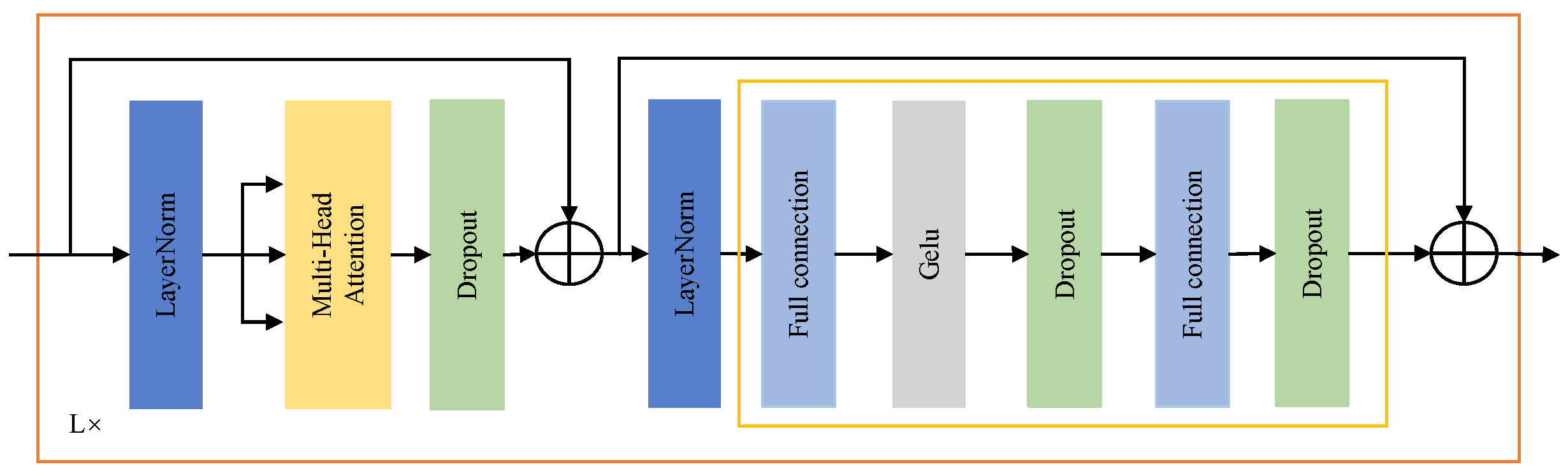
The transformer encoder, which is the kernel structure of this part, is shown in
Figure 5. The transformer encoder is composed of multiple layers, and each layer contains two residual blocks, which mainly include the multi-head self-attention (MSA) unit and multi-layer perceptron (MLP) unit. Supposed there are
N layers in the transformer encoder, the details of these two residual blocks in each layer will be introduced below.
The first residual block is formed by adding the result of the input vector going through layer normalization (LN) [
34] and MSA unit to itself. LN is used to implement normalization. Different from the commonly used batch normalization (BN), all the hidden units in a layer share the same normalization terms under LN. Thus, LN does not impose any constraint on the size of a mini-batch. MSA, the core of the transformer encoder, is to calculate the correlation as a weight by multiplying the query and the key and then using this weight to weighted sum the value to increase the weight of related elements in a sequence and reduce the weight of irrelevant elements.
Here the calculation process of the first residual block is described. Suppose
is the input of the first residual block on the
nth layer of the transformer encoder, and
is the output. Among them,
k is the number of images in a multi-aspect SAR image sequence,
m represents the channel number of each image’s feature vectors, and the input of the first layer is the output of the position-embedding
. The input vector
first passes through LN to get
; that is:
where
indicates the process of LN. Then,
is divided into
H parts along the channel dimension. Suppose
, each part is recorded as
,
, and corresponds to a head of self-attention. In other words,
, where
H is the number of heads in MSA. For each head, the input
is multiplied by three learnable matrices, the query matrix
, the key matrix
and the value matrix
to obtain the query vector
, the key vector
and the value vector
, which can be formulated as:
Then, the transposed matrix of
and
are multiplied to obtain the initial correlation matrix
, and then a softmax operation is performed on
column by column to obtain the correlation matrix
. The calculation process is written as:
is multiplied by the weight matrix
to get the output
; that is:
Then, the output vectors of each head
,
are concatenated along the channel dimension to obtain
. The output of MSA
is obtained by multiplying
with a trainable matrix
; that is
. Finally, to get the output of the first residual block
, the residual operation is applied to compute the summation of this block
and the output of MSA
, which can be formulated as:
The second residual block of each layer in the transformer encoder is composed of adding the results of the input vector through MLP to itself. The input vector of the second residual block
goes through LN, a fully connected sublayer with the nonlinear activation function and another fully connected sublayer in turn. The two fully connected sublayers expand and restore the vector dimension, respectively, thereby enhancing the expressive ability of the model. The number of neurons of the two fully connected sublayers is
and
m, respectively. GELU is employed as the activation function, which performs well in transformer-based networks, and its definition is given as follows:
where
is the cumulative distribution function of the standard normal distribution. Finally, through the residual operation, the output of the second residual block
, which is also the output of the
layer of the transformer encoder, is obtained. The calculation process of the second residual block is described as:
where
represent the operation of the two fully connected sublayers separately.
To alleviate the overfitting issue that is prone to occur when the training sample is insufficient, dropout is added at the end of each fully connected sublayer. Dropout is implemented by ignoring part of the hidden layer nodes in each training batch, and to put it simply, p percent neurons in the hidden layer stop working during each training iteration.
2.5. Feature Dimensionality Reduction
After the multi-aspect feature learning process based on self-attention, features that contain intrinsic correlation information of multi-aspect SAR image sequence have been extracted with the size of . Before using these features for classification, their dimension needs to be reduced.
MLP is the most commonly used feature dimensionality reduction method but one that lacks cross-channel information integration. Our proposed method uses a
convolution [
35] for dimensionality reduction, which uses the
convolution kernel and adjusts the feature dimension by the number of convolution kernels. The
convolution realizes the combination of information between channels, thus reducing the loss of information during dimensionality reduction. At the same time, compared with MLP, the
convolution reduces the number of parameters.
The input of the
convolutional layer is the output of the transformer encoder
, and the output size is
, where
C is the number of classes. Therefore, the number of convolution kernels of the
convolution layer is
C. Before the convolution operation, dimension transformation is performed from
to
. Suppose the output of dimensionality reduction is
,
is the convolution kernel of the
convolutional layer and
is the bias. The dimensionality reduction process is described as:
After dimensionality reduction, dimensional transformation is performed on
to obtain
for subsequent classification.
2.6. Classification
The classification process uses the softmax classifier. After dimensionality reduction, Z is averaged along the sequence dimension to get . Finally, the softmax operation is appiled upon to get the probability output .
2.7. Training Process
2.7.1. Pre-Train of CAE and Layer Transfer
CAE is an unsupervised learning method. As described in
Section 2.3, taking the single-aspect SAR images as input, after the forward propagation, reconstructed images will be obtained. Network optimization of CAE is achieved by minimizing the mean square error (MSE) between the reconstructed image and the original image; that is, using the MSE loss function. Suppose the total number of samples is
.
x is the input image, and
is the reconstructed image. The MSE loss function is defined as
In this work, backpropagation (BP) is selected to minimize the loss function and optimize the CAE parameters. The aim of BP is to calculate the gradient and update the network parameters to achieve the global minimum of the loss function. The process of BP is to calculate the error of each parameter from the output layer to the input layer through the chain rule, which is related to the partial derivative of the loss function relative to the trainable parameters, and then the parameters are updated according to the gradient. When the network converges, it means that the encoder of CAE can extract enough information to reconstruct the single-aspect SAR image, which can prove the effectiveness of feature extraction.
After the CAE network converges, the parameters of the encoder are saved for subsequent layer transfer. The specific layer transfer operation is first when initializing network parameters; the CNN for feature extraction loads the parameters of the trained encoder of CAE. Next, in the process of network training, the parameters of each layer of the CNN can be frozen, which means that they will remain unchanged during the training process or continue to be optimized; that is, fine-tuning. It should be noted that only the first two layers of the CNN are frozen, and the last layer of the CNN is fine-tuned along with the overall network in our method. This is because the pre-training of CAE is carried out for single-aspect SAR images. Therefore, in order to effectively extract sufficient internal correlation information to support multi-aspect feature learning, it is necessary to fine-tune during the whole network training. At the same time, the parameters of the first two layers are frozen to maintain the effective extraction of the main features of each single-aspect image to ensure the noise resistance of the network.
2.7.2. Training of Overall Network
Taking the multi-aspect SAR image sequence as input, after the forward propagation, the predicted results given by the proposed network will be obtained. Network optimization is achieved by minimizing the cross entropy between data labels and the predicted result given by the network; that is, using the cross entropy loss function. Suppose the total number of the sequence samples is
. For the
sample, let
denote the label, and
represent the probability output predicted by the network. When the sample belongs to the
class,
and
(
). Then the cross entropy loss function can be written as:
The proposed method also minimizes the loss function and optimizes the network parameters by BP, which is the same as most SAR ATR methods. The parameter updating in the BP process is affected by the learning rate, which determines how much the model parameters are adjusted according to the gradient in each parameter update. In the early stage of network training, there is a large difference between the network parameters and the optimal solution. Thus the gradient descent can be carried out faster with a larger learning rate. However, in the later stage of network training, gradually reducing the value of the learning rate will help the convergence of the network and make the network’s approach to the optimal solution easier. Therefore, in this work, the learning rate is decreased by piecewise constant decay.
3. Experiments and Results
To verify the effectiveness of our proposed method, first, the network architecture setup is specified, and then the multi-aspect SAR image sequences are constructed using the MSTAR dataset under the standard operating condition (SOC) and extended operating condition (EOC), respectively. Finally, the performance of the proposed method has been extensively assessed by conducting experiments under different conditions.
3.1. Network Architecture Setup
In the experiment, the network instances were deployed whose input can be single-aspect images or multi-aspect sequences to comprehensively evaluate the recognition performance of the network. In this instance, the size of the input SAR image is . The encoder of CAE includes three convolution-maxpooling layers, which obtain 64, 64 and 256 feature maps, respectively. In each layer, the convolution operation with kernel size and stride size is followed by the max-pooling operation with kernel size and stride size . The decoder of CAE includes three unpooling-deconvolution layers with the number of channels 64, 64 and 1, respectively. In each layer, the unpooling operation with kernel size and stride size is followed by the deconvolution operation with kernel size and stride size . In the transformer encoder with 6 layers, MSA has 4 heads and the number of neurons of the 2 fully connected sublayers is 512 and 256 in turn.
Our proposed network is implemented by the deep learning toolbox Pytorch 1.9.1. All the experiments are conducted on a PC with an Intel Core i7-9750H CPU at 2.60 GHz, 16.0 G RAM, and a NVIDIA GeForce RTX 2060 GPU. The learning rate is when training CAE and starts from with decay rate 0.9 every 30 epochs when training the whole network. The mini-batch size is set to 32, and the probability of dropout is 0.1.
3.2. Dataset
The MSTAR dataset [
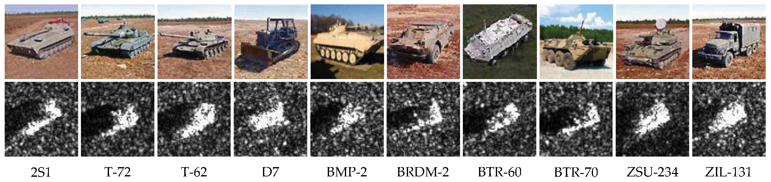
36], which was jointly released by the U.S. Defense Advanced Research Projects Agency (DARPA) and the U.S. Air Force Research Laboratory (AFRL), consists of high-quality SAR image data collected from ten stationary military vehicles (i.e., rocket launcher: 2S1; tank: T72 and T62; bulldozer: D7; armored personnel carrier: BMP2, BRDM2, BTR60 and BTR70; air defense unit: ZSU234; truck: ZIL131 ) through the X-band high-resolution Spotlight SAR by Sandia National Laboratory between 1996 and 1997. All images in the MSTAR dataset have a resolution of
with HH polarization. The azimuth aspect range of imaging each target covers
∼
with an interval of
∼
. The optical images of ten targets and their corresponding SAR images are illustrated in
Figure 6.
The acquisition conditions of the MSTAR dataset include two categories: Standard Operating Condition (SOC) and Extended Operating Condition (EOC). Specifically, SOC refers to the images of the training set and testing set that have the same target type and similar imaging configuration. Compared with SOC, the data of the training set and testing set of EOC are more different and have greater difficulty in identification. Generally, the EOC includes configuration-variant (EOC-C) and version-variant EOC (EOC-V).
First, the images are cropped to
and normalized. Next, the experiments are conducted using the sequences constructed according to the steps described in
Section 2.2 under SOC and EOC and the results are shown in
Section 3.3 and
Section 3.4. Then, the performance of the proposed method is compared with other existing methods in
Section 3.5. Finally, some further discussions are shown in
Section 3.6 about the influence of convolution kernel size in feature extraction and the performance of the network with few samples and noise.
3.3. Results under SOC
SOC means that the training and test datasets have the same target type and similar imaging configuration. The experiment under SOC is a classical ten-class classification problem of vehicle targets. Among the raw SAR images, the images collected at
depression angle are set as the training set, and the SAR images collected at
depression angle as the testing set. By applying the method of constructing sequences described in
Section 2.2, the training sequences and testing sequences are obtained when the angle range is set as
as in other multi-aspect SAR ATR methods, considering the actual radar imaging situation and the tradeoff between the cost of data acquisition and network training [
28].
Table 1 shows the class types and the number of training samples and test samples used in the experiment when the sequence length is set to 2, 3 and 4, respectively.
Table 2 shows the classification confusion matrix when the input is a single-aspect image as control, and
Table 3,
Table 4 and
Table 5 show the confusion matrix when each input sequence sample contains 2, 3 and 4 images, respectively. Confusion matrix is widely used in SAR target recognition to evaluate the recognition performance of the method. Each element of the confusion matrix represents the number of samples of each class recognized as a certain class. The rows of the confusion matrix correspond to the actual class of the target, and the columns show the class predicted by the network.
From
Table 3,
Table 4 and
Table 5, it can be observed that the recognition rate of our proposed method with 2, 3 and 4-aspect SAR image input sequences are all higher than 99.00% under SOC in the ten-class problem. Compared with the recognition rate shown in
Table 2, it is proven that the multi-aspect SAR image sequence contains more recognition information than the single-aspect SAR image. In addition, from the improvement of the recognition rate in
Table 3,
Table 4 and
Table 5 from 99.35%, 99.46% to 99.90%, it can be concluded that the self-attention process of our proposed method can effectively extract more internal correlation information of multi-aspect SAR images, so as to improve the recognition rates with the increase in the sequence length of multi-aspect SAR image sequence samples.
3.4. Results under EOC
Compared with SOC, the experiment under EOC is more difficult for target recognition due to the structure difference between the training set and testing set, which is often used to verify the robustness of the target recognition network. The experiments under EOC mainly include two experimental schemes, configuration variation (EOC-C) and version variation (EOC-V).
According to the original definition, EOC-V refers to targets of the same class that were built to different blueprints, while EOC-C refers to targets that were built to the same blueprints but had different post-production equipment added. The training sets under EOC-C and EOC-V are the same, which consist of four classes of targets (BMP2, BRDM2, BTR70 and T72), and the depression angle is
. The testing set under EOC-C consists of images of two classes of targets (BMP2 and T72) with seven different configuration variations acquired at both
and
depression angles, and the testing set under EOC-V consists of images of T72 with five different version variations acquired at both
and
depression angles. The training and testing samples for the experiment under EOC-C and EOC-V are listed in
Table 6,
Table 7 and
Table 8.
The confusion matrices of experiments under EOC-C and EOC-V with single-aspect input images, 2, 3 and 4-aspect input sequences are summarized in
Table 9 and
Table 10, respectively.
Table 9 shows the superior recognition performance of the proposed network in identifying BMP2 and T72 targets with configuration differences. The recognition rates of the proposed method reach 96.91%, 97.66% and 98.50% with 2, 3 and 4-aspect input sequences, respectively, which are all higher than 94.65% for the single-aspect input image. It can prove that, under EOC-C, the network can still learn more recognition information from multi-aspect images through self-attention so as to obtain better recognition performance.
Table 10 shows the excellent performance of the proposed network in identifying T72 targets with version differences. With the increase in the input sequence length, the recognition rate of the network rises as well, from 98.12% for single-aspect input to 99.78% for four-aspect input.
The above experiments indicate that the proposed network can achieve a high recognition rate when tested under different operating conditions, which confirms the application value of the proposed network in actual SAR ATR tasks.
3.5. Recognition Performance Comparison
In this section, our proposed network is compared with six other methods, i.e., joint sparse representation (JSR) [
37], sparse representation-based classification (SRC) [
38], data fusion [
39], multiview deep convolutional neural network (MVDCNN) [
28], bidirectional convolutional-recurrent network (BCRN) [
27] and multiview deep feature learning network (MVDFLN) [
29], which have been widely cited or recently published in SAR ATR. Among them, the first three are classical multi-aspect SAR ATR methods. JSR and SRC are two classical methods based on sparse representation, and data fusion refers to the fusion of multi-aspect features based on principal component analysis (PCA) and discrete wavelet transform (DWT). The last three are all deep learning multi-aspect SAR ATR methods.
Here, first, the recognition performance under SOC and EOC is compared between these methods. The recognition rates for each method under SOC and EOC are listed in
Table 11. It should be noted that in order to objectively evaluate the performance of the method, it should be ensured that the datasets are as much the same as possible. Among the six methods, the original BCRN uses the image sequences with a sequence length of 15 as the input, which contains more identification information and requires a larger computational burden. That is, the original BCRN is difficult to compare with the other methods with an input sequence length of 3 or 4. Therefore, BCRN is implemented, and the results in
Table 11 are obtained using the same four-aspect training and testing sequences as our method.
From
Table 11, it is obvious that our method has a higher recognition rate than the other six methods in multi-aspect SAR ATR tasks, which proves that the combination of CNN and self-attention can learn the recognition information more effectively in multi-aspect SAR target recognition.
Then, as shown in
Table 12, compared with BCRN, our method greatly reduces the model size; that is, it greatly reduces the number of parameters and is in the same order of magnitude as MVDCNN. Considering the network structure of MVDCNN, when the sequence length increases, the network depth and the number of parallel branches will increase correspondingly. On the contrary, our method does not change the network structure when the sequence length increases, so it is more flexible, and the number of parameters increases slowly with the sequence length. As for the FLOPs, which represent the speed of network reasoning, it can be seen that our method still needs to be optimized. It is speculated that the amount of floating point operations mainly comes from the large convolution kernels for feature extraction and matrix operations for self-attention.
3.6. Discussion
For further discussion, the experiments on the network structure of feature extraction are carried out first. In order to obtain 1-D feature vectors, when a smaller convolution kernel is selected, the number of layers of CNN will increase accordingly. The recognition rates compared between the 6-layer CNN for feature extraction with the convolution kernel size of
and 3-layer CNN with the kernel size of
are shown in
Table 13. From the results under EOC, it can be seen that the recognition performance of the larger convolution kernel network is better. Such a result is obtained because the larger convolution kernel can better extract the global information in raw images, which is beneficial to self-attention to learn common features in image sequences as a basis for classification. On the contrary, small convolution kernels are more concentrated on local information, which varies greatly from different angles.
When the number of transformer encoder layers is different, the recognition performance of the whole network will also be different. The recognition accuracy under different operating conditions with different transformer encoder layers is shown in
Table 14. When the transformer encoder has more layers, it means that the self-attention calculation has been carried out more times, so it is possible to mine more correlation information, which is also confirmed by the higher recognition accuracy achieved in the experiment.
Next, in order to verify the recognition ability of the method with few samples, the training sequence is downsampled and the recognition rates of BCRN and MVDCNN are compared with our method when the number of training sequences is 50%, 25%, 10%, 5% and 2% of the original under SOC. As shown in
Table 15, the recognition accuracy only decreases by 5% when the number of training sequence samples decreases to 2%, which is much less than 21.8% for BCRN and 11.03% for MVDCNN. As is known to all, the transformer needs a lot of data for training, which is mainly due to the lack of prior experience contained in the convolution structure, such as translation invariance and locality [
30]. In our proposed method, we use CNN to extract features first so as to make up for the lost local information. Therefore, the network also has excellent performance in the case of few samples.
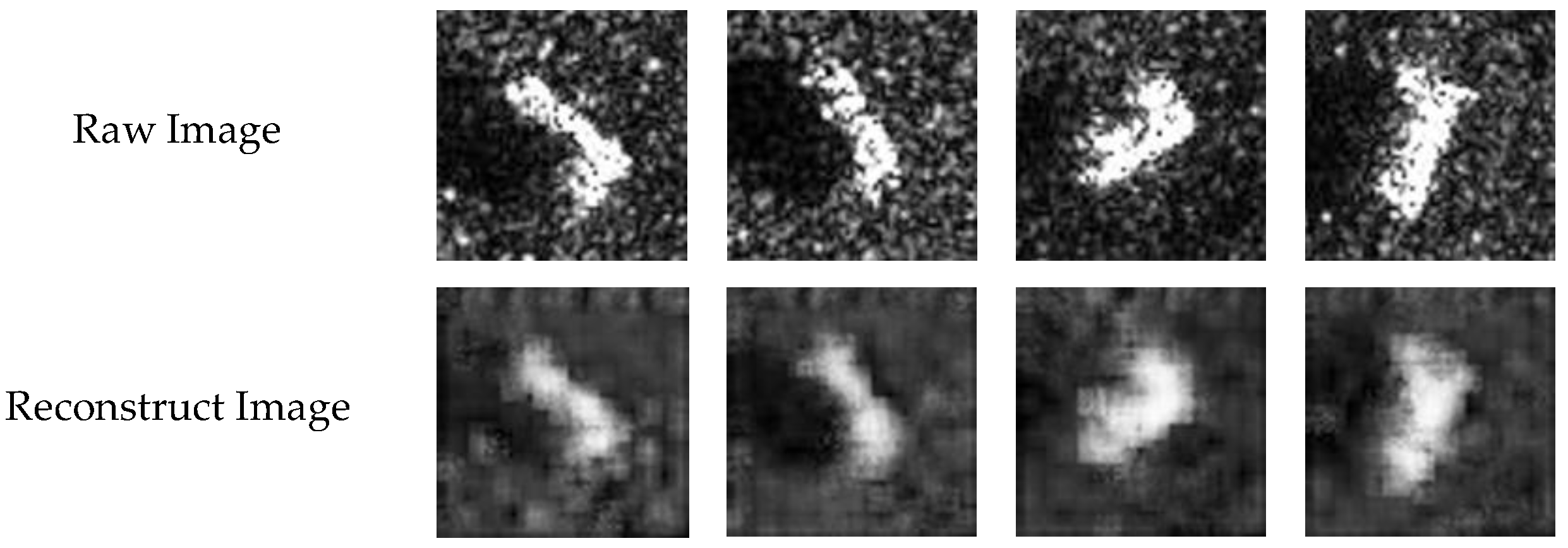
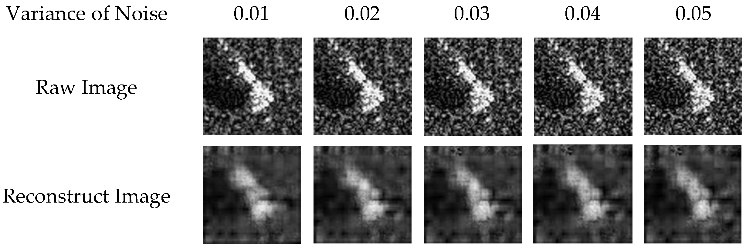
Finally, considering that in actual SAR ATR tasks, SAR images often contain noise, which has a great impact on the performance of SAR ATR because of the sensitivity of SAR images to noise, experiments are carried out to test the anti-noise performance of the network under SOC. As shown in
Figure 7, the output of input image reconstruction by convergent CAE can reflect the main characteristics of the target in the input image but blur some other details. This indicates that when the image contains noise, the feature extraction network can filter the noise and extract the main features of the target. This is proven by the test image with noise with variance from 0.01 to 0.05 and the results of its convergent CAE reconstruction shown in
Figure 8.
Table 16 shows the recognition rates of the methods to be compared when the variance of noise increases from 0.01 to 0.05. Obviously, after pre-training, our method has excellent anti-noise ability. When the input image is seriously polluted by noise, the recognition rate of BCRN and the network without CAE is low, but the proposed method with CAE still maintains a high recognition rate, which shows that CAE plays an important role in anti-noise.
In addition, to further verify the effectiveness of the pre-trained CAE, as shown in
Table 17, CAE is replaced by other structures for experimental comparison. DS-Net [
40] in the table is a feature extraction structure composed of dense connection and separable convolution. The experimental results show that compared with other structures, the proposed method with CAE does show better recognition performance under a variety of complex conditions, which proves the advantage of CAE in extracting major features.


