


Exploring the Individualized Effect of Climatic Drivers on MODIS Net Primary Productivity through an Explainable Machine Learning Framework


Abstract
:
1. Introduction
2. Methodology
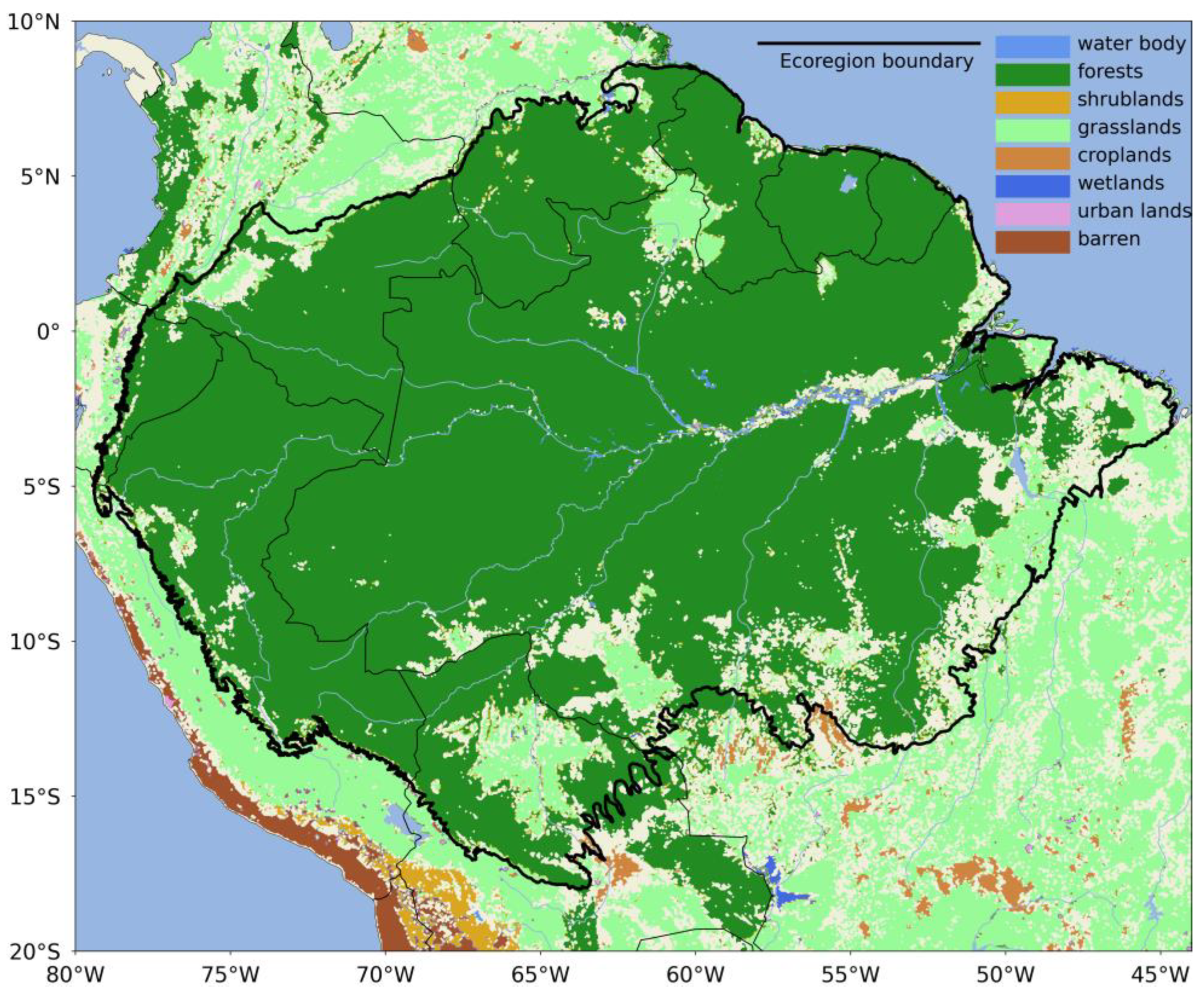
2.1. Study Area
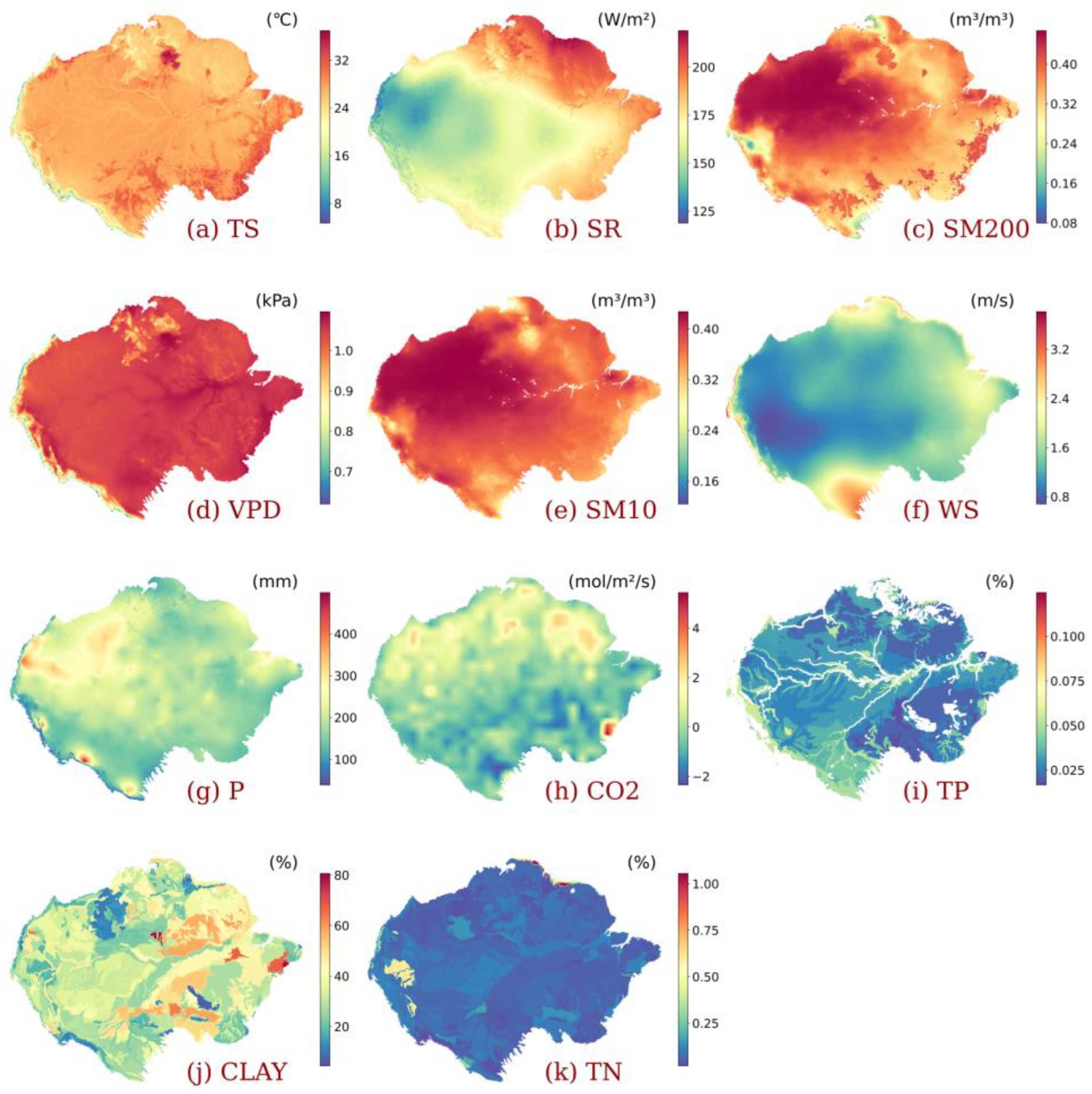
2.2. Data
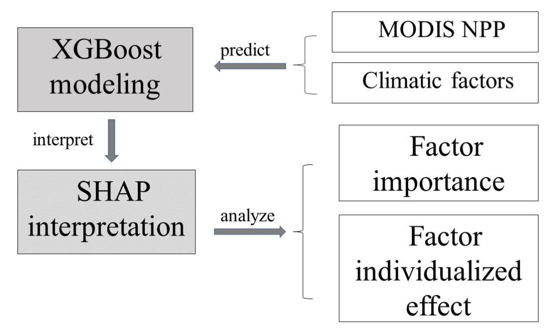
2.3. Machine Learning Model
2.4. Model Interpretation
3. Results
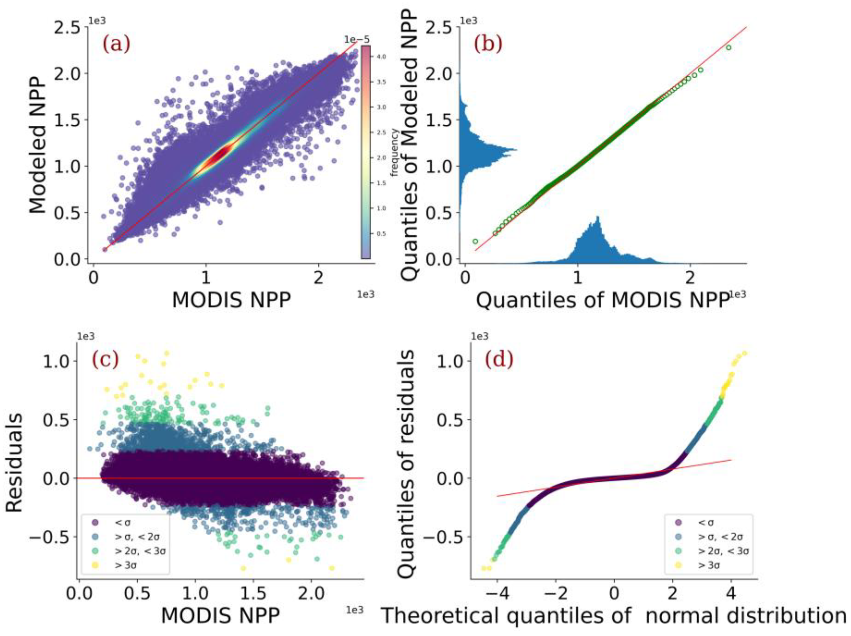
3.1. Model Evaluation
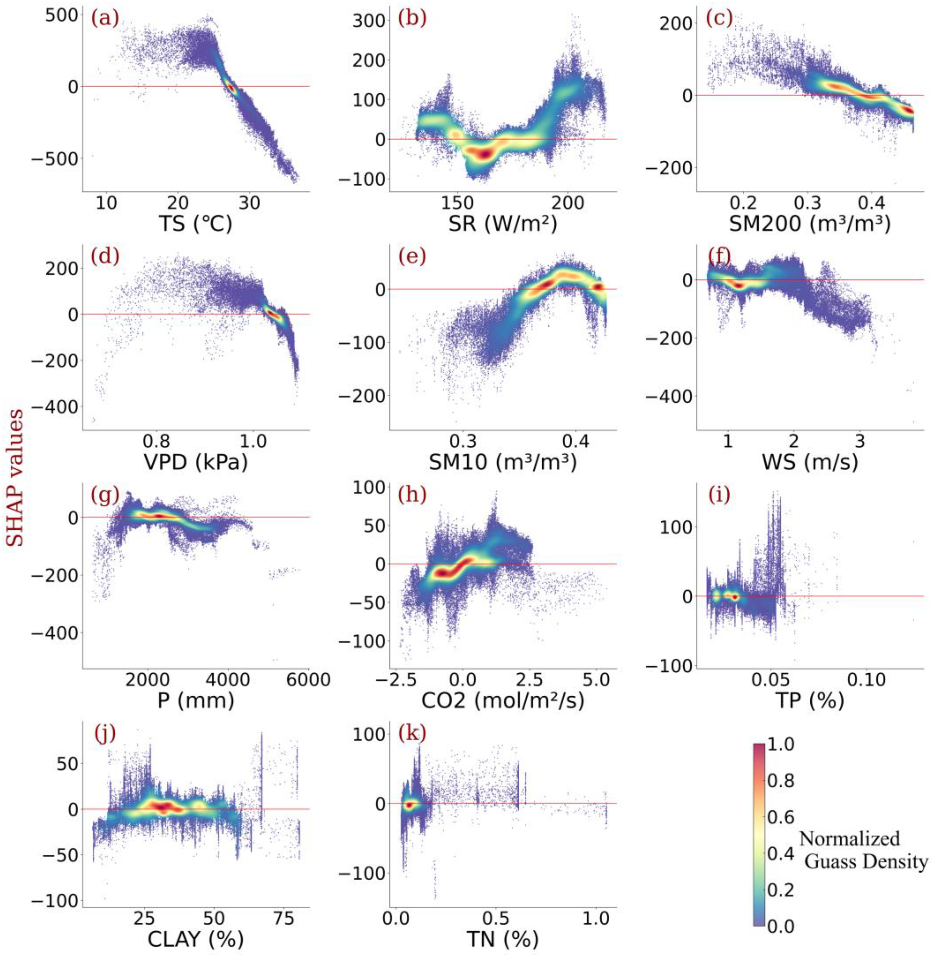
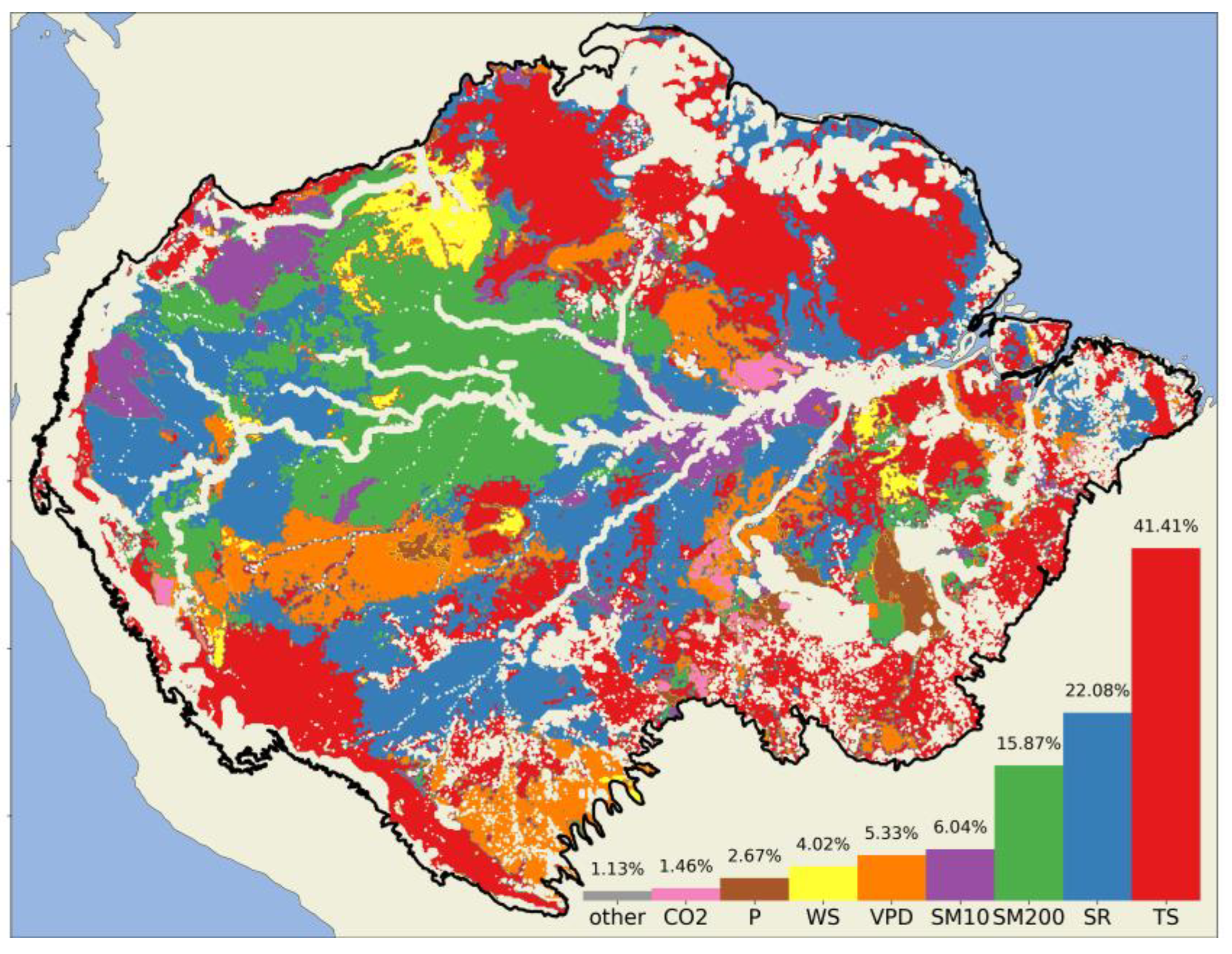
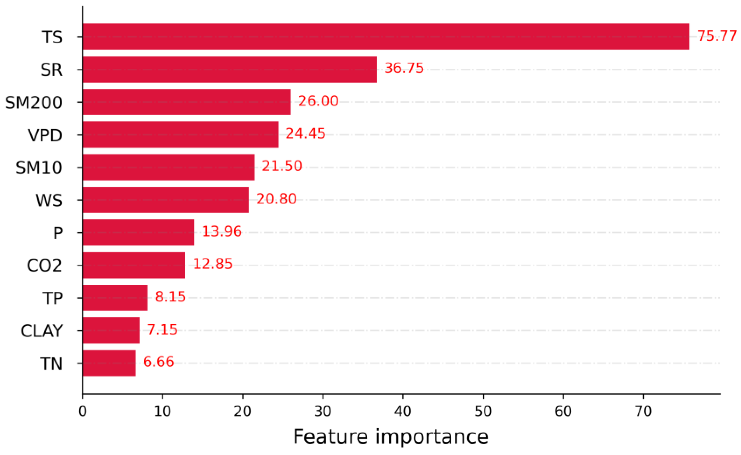
3.2. Relative Importance of Drivers of NPP
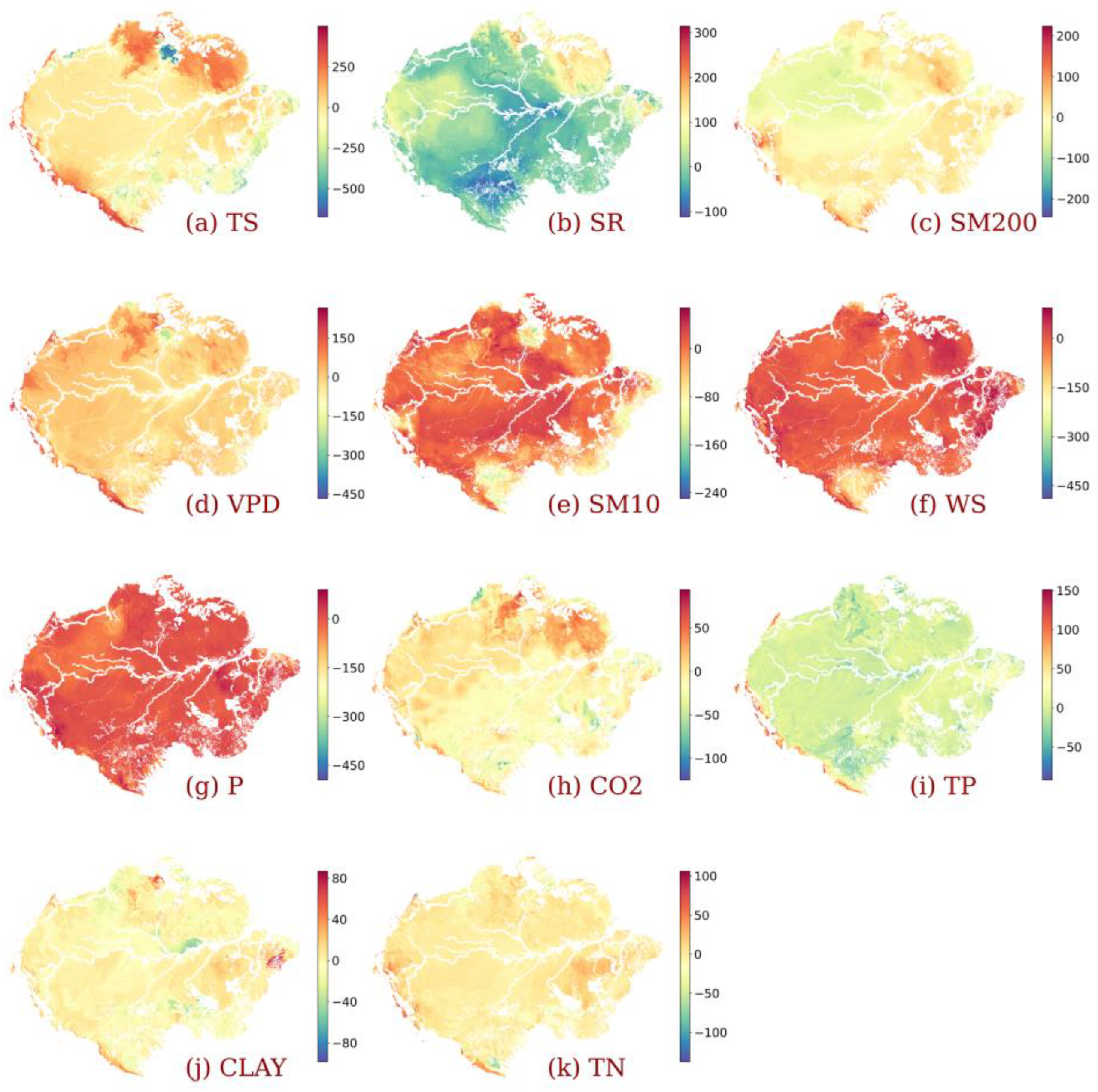
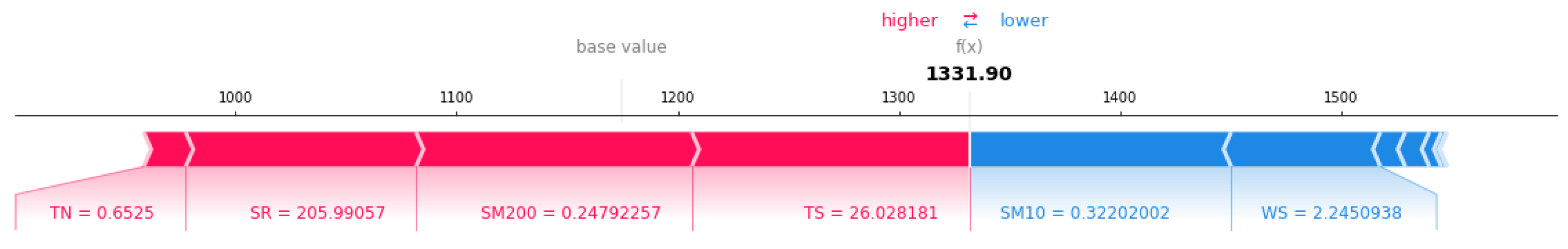
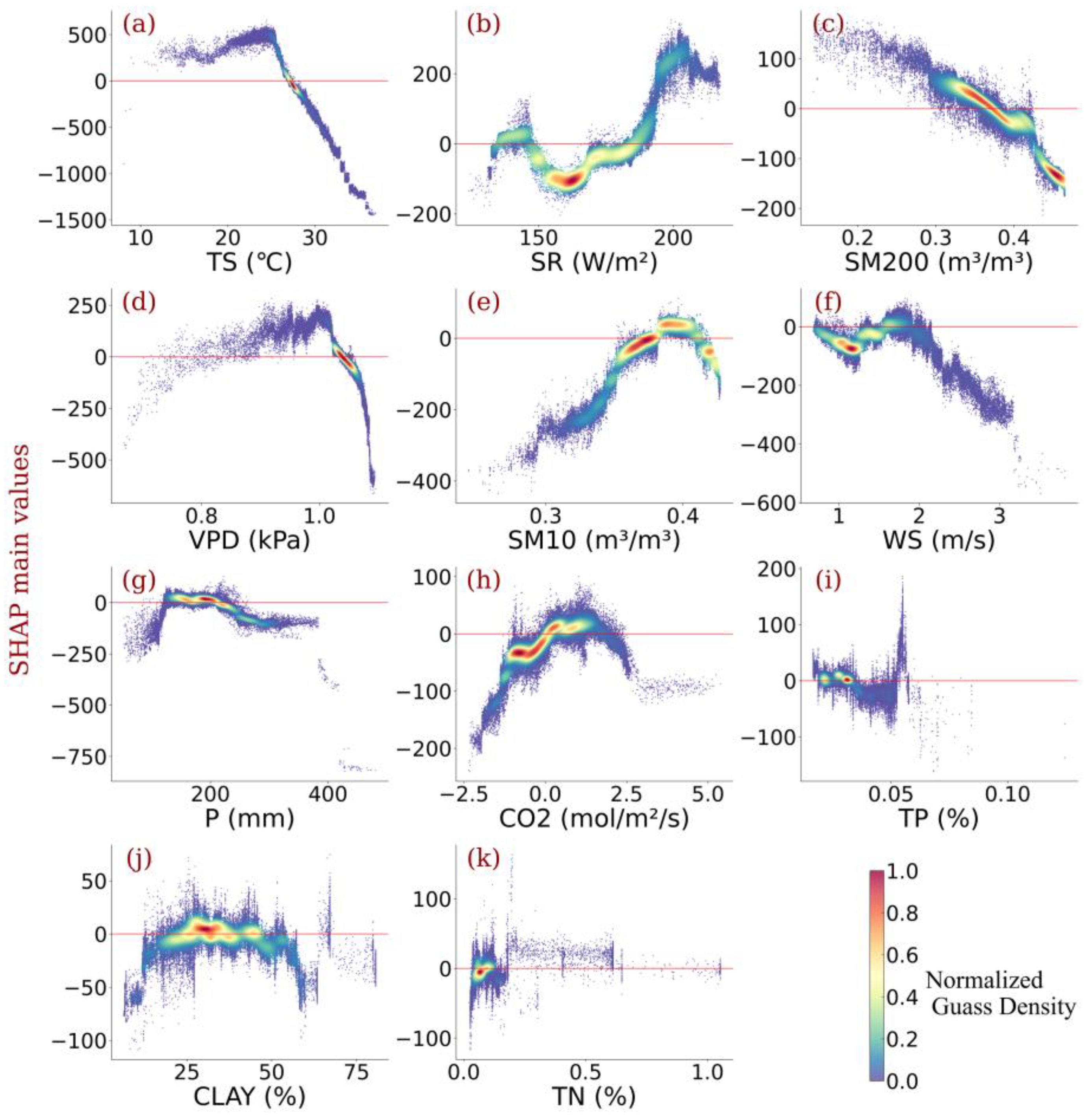
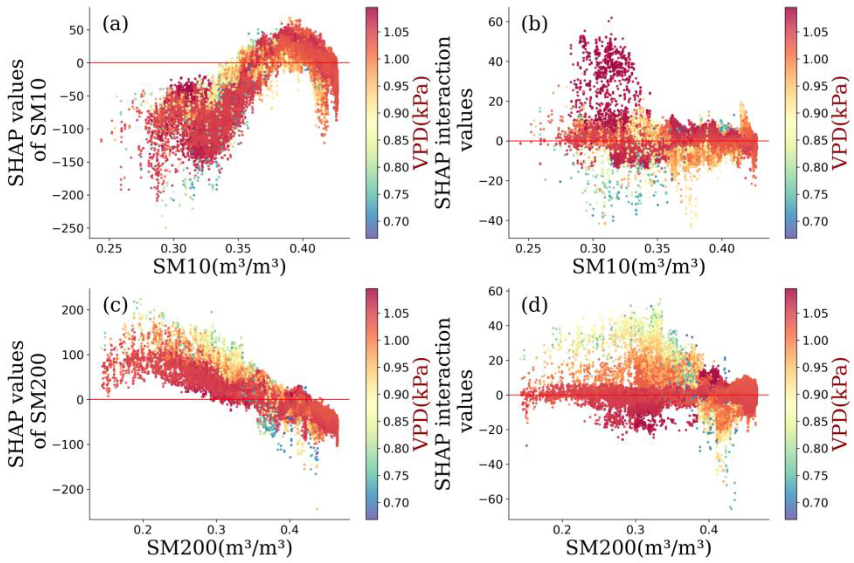
3.3. Impact of Individualized Climatic Drivers on Spatial Variability of NPP
4. Discussion
4.1. Dominant Drivers of Spatial Variability of Amazonia NPP
4.2. Amazonia Vegetation Responds to Moisture
4.3. Benefits and Uncertainty of Explainable Machine Learning
5. Conclusions
- Relative contributions of each driver were identified, showing that the temperature outperformed other climatic variables in contributing to Amazonia NPP variability. Radiation and vapor pressure deficit also made a considerable contribution. Wind speed, CO2 concentration, and precipitation were also responsible.
- Individualized feature attribution was detected. In most areas of Amazon forests, the temperature exceeded the optimal value for NPP growth. Generally, elevated radiation and increased CO2 concentration promote NPP gain monotonically, while high precipitation impairs NPP. In addition, for most vegetation, the wind speed did not reach the optimum value that benefits NPP, and sustained high wind speed would bring substantial NPP loss.
- Amazonia NPP responded to VPD non-monotonically. Considering the distinct response of NPP to soil water content under different layers, the relationship between NPP and VPD was highly connected to the water use policy and moisture overload conditions in Amazon forests. Further increases in VPD largely impaired NPP despite the moisture overload conditions in Amazon forests.
Author Contributions
Funding
Data Availability Statement
Acknowledgments
Conflicts of Interest
Appendix A

References
- Bonan, G.B.; Doney, S.C. Climate, ecosystems, and planetary futures: The challenge to predict life in Earth system models. Science 2018, 359, 533. [Google Scholar] [CrossRef]
- Lovenduski, N.S.; Bonan, G.B. Reducing uncertainty in projections of terrestrial carbon uptake. Environ. Res. Lett. 2017, 12. [Google Scholar] [CrossRef]
- Hansen Matthew, C.; Stehman Stephen, V.; Potapov Peter, V. Quantification of global gross forest cover loss. Proc. Natl. Acad. Sci. USA 2010, 107, 8650–8655. [Google Scholar] [CrossRef]
- Pan, Y.; Birdsey, R.A.; Fang, J.; Houghton, R.; Kauppi, P.E.; Kurz, W.A.; Phillips, O.L.; Shvidenko, A.; Lewis, S.L.; Canadell, J.G.; et al. A Large and Persistent Carbon Sink in the World’s Forests. Science 2011, 333, 988–993. [Google Scholar] [CrossRef]
- Field, C.B.; Behrenfeld, M.J.; Randerson, J.T.; Falkowski, P. Primary Production of the Biosphere: Integrating Terrestrial and Oceanic Components. Science 1998, 281, 237–240. [Google Scholar] [CrossRef]
- Chu, C.; Bartlett, M.; Wang, Y.; He, F.; Weiner, J.; Chave, J.; Sack, L. Does climate directly influence NPP globally? Glob. Chang. Biol. 2016, 22, 12–24. [Google Scholar] [CrossRef]
- De Jong, R.; Schaepman, M.E.; Furrer, R.; De Bruin, S.; Verburg, P.H. Spatial relationship between climatologies and changes in global vegetation activity. Glob. Chang. Biol. 2013, 19, 1953–1964. [Google Scholar] [CrossRef]
- Chu, C.; Lutz, J.A.; Král, K.; Vrška, T.; Yin, X.; Myers, J.A.; Abiem, I.; Alonso, A.; Bourg, N.; Burslem, D.F.; et al. Direct and indirect effects of climate on richness drive the latitudinal diversity gradient in forest trees. Ecol. Lett. 2019, 22, 245–255. [Google Scholar] [CrossRef]
- Craine, J.M.; Nippert, J.B.; Elmore, A.J.; Skibbe, A.M.; Hutchinson, S.L.; Brunsell, N.A. Timing of climate variability and grassland productivity. Proc. Natl. Acad. Sci. USA 2012, 109, 3401–3405. [Google Scholar] [CrossRef]
- Beer, C.; Reichstein, M.; Tomelleri, E.; Ciais, P.; Jung, M.; Carvalhais, N.; Rödenbeck, C.; Arain, M.A.; Baldocchi, D.; Bonan, G.B.; et al. Terrestrial gross carbon dioxide uptake: Global distribution and covariation with climate. Science 2010, 329, 834–838. [Google Scholar] [CrossRef] [Green Version]
- Bonan, G.B. Forests and climate change: Forcings, feedbacks, and the climate benefits of forests. Science 2008, 320, 1444–1449. [Google Scholar] [CrossRef]
- Nemani, R.R.; Keeling, C.D.; Hashimoto, H.; Jolly, W.M.; Piper, S.C.; Tucker, C.J.; Myneni, R.B.; Running, S.W. Climate-Driven Increases in Global Terrestrial Net Primary Production from 1982 to 1999. Science 2003, 300, 1560–1563. [Google Scholar] [CrossRef] [PubMed]
- Running, S.W.; Nemani, R.R.; Heinsch, F.A.; Zhao, M.S.; Reeves, M.; Hashimoto, H. A Continuous Satellite-Derived Measure of Global Terrestrial Primary Production. Bioscience 2004, 54, 547–560. [Google Scholar] [CrossRef]
- Churkina, G.; Running, S.W. Contrasting Climatic Controls on the Estimated Productivity of Global Terrestrial Biomes. Ecosystems 1998, 1, 206–215. [Google Scholar] [CrossRef]
- Zhou, H.; Shao, J.; Liu, H.; Du, Z.; Zhou, L.; Liu, R.; Bernhofer, C.; Grünwald, T.; Dušek, J.; Montagnani, L.; et al. Relative importance of climatic variables, soil properties and plant traits to spatial variability in net CO2 exchange across global forests and grasslands. Agric. For. Meteorol. 2021, 307. [Google Scholar] [CrossRef]
- Li, P.; Peng, C.; Wang, M.; Li, W.; Zhao, P.; Wang, K.; Yang, Y.; Zhu, Q. Quantification of the response of global terrestrial net primary production to multifactor global change. Ecol. Indic. 2017, 76, 245–255. [Google Scholar] [CrossRef]
- Yuan, W.; Zheng, Y.; Piao, S.; Ciais, P.; Lombardozzi, D.; Wang, Y.; Ryu, Y.; Chen, G.; Dong, W.; Hu, Z.; et al. Increased atmospheric vapor pressure deficit reduces global vegetation growth. Sci. Adv. 2019, 5, eaax1396. [Google Scholar] [CrossRef] [PubMed]
- Wang, S.; Zhang, Y.; Ju, W.; Chen, J.M.; Ciais, P.; Cescatti, A.; Sardans, J.; Janssens, I.A.; Wu, M.; Berry, J.A.; et al. Recent global decline of CO2 fertilization effects on vegetation photosynthesis. Science 2021, 371. [Google Scholar] [CrossRef]
- Song, Y.; Jiao, W.Z.; Wang, J.; Wang, L.X. Increased Global Vegetation Productivity Despite Rising Atmospheric Dryness Over the Last Two Decades. Earths Future 2022, 10. [Google Scholar] [CrossRef]
- Chen, R.N.; Liu, L.Y.; Liu, X.J. The Negative Impact of Excessive Moisture Contributes to the Seasonal Dynamics of Photosynthesis in Amazon Moist Forests. Earths Future 2022, 10. [Google Scholar] [CrossRef]
- Green, J.K.; Berry, J.; Ciais, P.; Zhang, Y.; Gentine, P. Amazon rainforest photosynthesis increases in response to atmospheric dryness. Sci. Adv. 2020, 6, eabb7232. [Google Scholar] [CrossRef] [PubMed]
- Chen, N.; Song, C.; Xu, X.; Wang, X.; Cong, N.; Jiang, P.; Zu, J.; Sun, L.; Song, Y.; Zuo, Y.; et al. Divergent impacts of atmospheric water demand on gross primary productivity in three typical ecosystems in China. Agric. For. Meteorol. 2021, 307, 108527. [Google Scholar] [CrossRef]
- Reichstein, M.; Camps-Valls, G.; Stevens, B.; Jung, M.; Denzler, J.; Carvalhais, N.; Prabhat. Deep learning and process understanding for data-driven Earth system science. Nature 2019, 566, 195–204. [Google Scholar] [CrossRef] [PubMed]
- Mittelstadt, B.; Russell, C.; Wachter, S. Explaining Explanations in AI. In Proceedings of the Conference on Fairness, Accountability, and Transparency, Atlanta, GA, USA, 29–31 January 2019; 2019; pp. 279–288. [Google Scholar]
- Besnard, S.; Koirala, S.; Santoro, M.; Weber, U.; Nelson, J.; Gütter, J.; Herault, B.; Kassi, J.; N’Guessan, A.; Neigh, C.; et al. Mapping global forest age from forest inventories, biomass and climate data. Earth Syst. Sci. Data 2021, 13, 4881–4896. [Google Scholar]
- Stirnberg, R.; Cermak, J.; Kotthaus, S.; Haeffelin, M.; Andersen, H.; Fuchs, J.; Kim, M.; Petit, J.-E.; Favez, O. Meteorology-driven variability of air pollution (PM1) revealed with explainable machine learning. Atmos. Chem. Phys. 2021, 21, 3919–3948. [Google Scholar] [CrossRef]
- Wang, H.; Yan, S.J.; Ciais, P.; Wigneron, J.P.; Liu, L.B.; Li, Y.; Fu, Z.; Ma, H.L.; Liang, Z.; Wei, F.L.; et al. Exploring complex water stress-gross primary production relationships: Impact of climatic drivers, main effects, and interactive effects. Glob. Chang. Biol. 2022, 28, 4110–4123. [Google Scholar] [CrossRef]
- Boisvenue, C.; Running, S.W. Impacts of climate change on natural forest productivity—Evidence since the middle of the 20th century. Glob. Chang. Biol. 2006, 12, 862–882. [Google Scholar] [CrossRef]
- Vitousek, P.M.; Ehrlich, P.R.; Ehrlich, A.H.; Matson, P.A. Net Primary Production: Original Calculations. Science 1987, 235, 730. [Google Scholar] [CrossRef]
- Olson, D.M.; Dinerstein, E.; Wikramanayake, E.D.; Burgess, N.D.; Powell, G.V.N.; Underwood, E.C.; D’Amico, J.A.; Itoua, I.; Strand, H.E.; Morrison, J.C.; et al. Terrestrial ecoregions of the worlds: A new map of life on Earth. Bioscience 2001, 51, 933–938. [Google Scholar] [CrossRef]
- Rödig, E.; Cuntz, M.; Heinke, J.; Rammig, A.; Huth, A. Spatial heterogeneity of biomass and forest structure of the Amazon rain forest: Linking remote sensing, forest modelling and field inventory. Glob. Ecol. Biogeogr. 2017, 26, 1292–1302. [Google Scholar] [CrossRef]
- Bauer, L.; Knapp, N.; Fischer, R. Mapping Amazon Forest Productivity by Fusing GEDI Lidar Waveforms with an Individual-Based Forest Model. Remote Sens. 2021, 13, 4540. [Google Scholar] [CrossRef]
- Running, S.; Mu, Q.; Zhao, M. MOD17A3H MODIS/Terra Net Primary Production Yearly L4 Global 500m SIN Grid V006; NASA EOSDIS Land Processes DAAC: Sioux Falls, SD, USA, 2015. [Google Scholar] [CrossRef]
- Zhao, M.; Heinsch, F.A.; Nemani, R.R.; Running, S.W. Improvements of the MODIS terrestrial gross and net primary production global data set. Remote Sens. Environ. 2005, 95, 164–176. [Google Scholar] [CrossRef]
- Fensholt, R.; Sandholt, I.; Rasmussen, M.S.; Stisen, S.; Diouf, A. Evaluation of satellite based primary production modelling in the semi-arid Sahel. Remote Sens. Environ. 2006, 105, 173–188. [Google Scholar] [CrossRef]
- Turner, D.P.; Ritts, W.D.; Cohen, W.B.; Gower, S.T.; Running, S.W.; Zhao, M.; Costa, M.H.; Kirschbaum, A.A.; Ham, J.M.; Saleska, S.R.; et al. Evaluation of MODIS NPP and GPP products across multiple biomes. Remote Sens. Environ. 2006, 102, 282–292. [Google Scholar] [CrossRef]
- Fu, Z.; Ciais, P.; Prentice, I.C.; Gentine, P.; Makowski, D.; Bastos, A.; Luo, X.; Green, J.K.; Stoy, P.C.; Yang, H.; et al. Atmospheric dryness reduces photosynthesis along a large range of soil water deficits. Nat. Commun. 2022, 13, 989. [Google Scholar] [CrossRef]
- Zhu, Z.; Piao, S.; Myneni, R.B.; Huang, M.; Zeng, Z.; Canadell, J.G.; Ciais, P.; Sitch, S.; Friedlingstein, P.; Arneth, A.; et al. Greening of the Earth and its drivers. Nat. Clim. Chang. 2016, 6, 791. [Google Scholar] [CrossRef]
- Wan, Z.; Hook, S.; Hulley, G. MODIS/Terra Land Surface Temperature/Emissivity Monthly L3 Global 0.05Deg CMG V061; NASA EOSDIS Land Processes DAAC: Sioux Falls, SD, USA, 2021. [Google Scholar] [CrossRef]
- Huang, M.; Piao, S.; Ciais, P.; Peñuelas, J.; Wang, X.; Keenan, T.F.; Peng, S.; Berry, J.A.; Wang, K.; Mao, J.; et al. Air temperature optima of vegetation productivity across global biomes. Nat. Ecol. Evol. 2019, 3, 772–779. [Google Scholar] [CrossRef]
- Abatzoglou, J.T.; Dobrowski, S.; Parks, S.A.; Hegewisch, K.C. TerraClimate, a high-resolution global dataset of monthly climate and climatic water balance from 1958–2015. Sci. Data 2018, 5, 170191. [Google Scholar] [CrossRef]
- McNally, A. FLDAS Noah Land Surface Model L4 Global Monthly 0.1 × 0.1 Degree (MERRA-2 and CHIRPS); Goddard Earth Sciences Data and Information Services Center (GES DISC): Greenbelt, MD, USA, 2018. [Google Scholar] [CrossRef]
- Howell, T.A.; Dusek, D.A. Comparison of Vapor-Pressure-Deficit Calculation Methods—Southern High Plains. J. Irrig. Drain. Eng. 2001, 127, 329–330. [Google Scholar] [CrossRef]
- Zhang, T.; Zhang, Y.; Xu, M.; Zhu, J.; Chen, N.; Jiang, Y.; Huang, K.; Zu, J.; Liu, Y.; Yu, G. Water availability is more important than temperature in driving the carbon fluxes of an alpine meadow on the Tibetan Plateau. Agric. For. Meteorol. 2018, 256, 22–31. [Google Scholar] [CrossRef]
- Jacobson, A.R.; Schuldt, K.N.; Miller, J.B.; Oda, T.; Tans, P.; Arlyn, A.; Mund, J.; Ott, L.; Collatz, G.J.; Aalto, T.; et al. CarbonTracker CT2019B; NOAA Earth System Research Laboratory, Global Monitoring Division: Bondville, IL, USA, 2020. [Google Scholar] [CrossRef]
- Shangguan, W.; Dai, Y.; Duan, Q.; Liu, B.; Yuan, H. A global soil data set for earth system modeling. J. Adv. Model. Earth Syst. 2014, 6, 249–263. [Google Scholar] [CrossRef]
- Friedl, M.; Sulla-Menashe, D. MCD12C1 MODIS/Terra+Aqua Land Cover Type Yearly L3 Global 0.05Deg CMG V006; NASA EOSDIS Land Processes DAAC: Sioux Falls, SD, USA, 2015. [Google Scholar] [CrossRef]
- Lundberg, S.M.; Erion, G.; Chen, H.; DeGrave, A.; Prutkin, J.M.; Nair, B.; Katz, R.; Himmelfarb, J.; Bansal, N.; Lee, S.-I. From local explanations to global understanding with explainable AI for trees. Nat. Mach. Intell. 2020, 2, 56–67. [Google Scholar] [CrossRef] [PubMed]
- Chen, T.Q.; Guestrin, C. XGBoost: A Scalable Tree Boosting System. In Proceedings of the 22nd Acm Sigkdd International Conference on Knowledge Discovery and Data Mining (Kdd’16), San Francisco, CA, USA, 13–17 August 2016; pp. 785–794. [Google Scholar] [CrossRef]
- Rossel, R.A.V.; Lee, J.; Behrens, T.; Luo, Z.; Baldock, J.; Richards, A. Continental-scale soil carbon composition and vulnerability modulated by regional environmental controls. Nat. Geosci. 2019, 12, 547. [Google Scholar] [CrossRef]
- Quinlan, J.R. Learning with Continuous Classes. In Proceedings of the 5th Australian Joint Conference on Artificial Intelligence, Hobart, Australia, 16–18 November 1992; Volume 10, pp. 475–476. [Google Scholar]
- Barnes, E.A.; Toms, B.; Hurrell, J.W.; Ebert-Uphoff, I.; Anderson, C.; Anderson, D. Indicator Patterns of Forced Change Learned by an Artificial Neural Network. J. Adv. Model. Earth Syst. 2020, 12. [Google Scholar] [CrossRef]
- Molina, M.J.; Gagne, D.J.; Prein, A.F. A Benchmark to Test Generalization Capabilities of Deep Learning Methods to Classify Severe Convective Storms in a Changing Climate. Earth Space Sci. 2021, 8. [Google Scholar] [CrossRef]
- Murdoch, W.J.; Singh, C.; Kumbier, K.; Abbasi-Asl, R.; Yu, B. Definitions, methods, and applications in interpretable machine learning. Proc. Natl. Acad. Sci. USA 2019, 116, 22071–22080. [Google Scholar] [CrossRef]
- Rasp, S.; Thuerey, N. Data-Driven Medium-Range Weather Prediction with a Resnet Pretrained on Climate Simulations: A New Model for WeatherBench. J. Adv. Model. Earth Syst. 2021, 13. [Google Scholar] [CrossRef]
- Lundberg, S.M.; Lee, S.I. A Unified Approach to Interpreting Model Predictions. Adv. Neural Inf. Process. Syst. 2017, 30. [Google Scholar] [CrossRef]
- Aas, K.; Jullum, M.; Løland, A. Explaining individual predictions when features are dependent: More accurate approximations to Shapley values. Artif. Intell. 2021, 298. [Google Scholar] [CrossRef]
- Shapley, L.S. Stochastic Games. Proc. Natl. Acad. Sci. USA 1953, 39, 1095–1100. [Google Scholar] [CrossRef]
- Strumbelj, E.; Kononenko, I. An Efficient Explanation of Individual Classifications using Game Theory. J. Mach. Learn. Res. 2010, 11, 1–18. [Google Scholar] [CrossRef]
- Štrumbelj, E.; Kononenko, I. Explaining prediction models and individual predictions with feature contributions. Knowl. Inf. Syst. 2014, 41, 647–665. [Google Scholar] [CrossRef]
- Lundberg, S.M.; Erion, G.G.; Lee, S.-I. Consistent Individualized Feature Attribution for Tree Ensembles. arXiv 2018, arXiv:1802.03888. [Google Scholar]
- LLi, H.; Zhang, F.; Li, Y.; Wang, J.; Zhang, L.; Zhao, L.; Cao, G.; Zhao, X.; Du, M. Seasonal and inter-annual variations in CO2 fluxes over 10 years in an alpine shrubland on the Qinghai-Tibetan Plateau, China. Agric. For. Meteorol. 2016, 228, 95–103. [Google Scholar] [CrossRef]
- Xu, M.J.; Wang, H.M.; Wen, X.F.; Zhang, T.; Di, Y.B.; Wang, Y.D.; Wang, J.L.; Cheng, C.P.; Zhang, W.J. The full annual carbon balance of a subtropical coniferous plantation is highly sensitive to autumn precipitation. Sci. Rep. 2017, 7. [Google Scholar] [CrossRef]
- Doughty, C.E.; Goulden, M.L. Are tropical forests near a high temperature threshold? J. Geophys. Res. Biogeogr. 2008, 113. [Google Scholar] [CrossRef] [Green Version]
- Phillips, O.L.; Aragao, L.E.O.C.; Lewis, S.L.; Fisher, J.B.; Lloyd, J.; Lopez-Gonzalez, G.; Malhi, Y.; Monteagudo, A.; Peacock, J.; Quesada, C.A.; et al. Drought Sensitivity of the Amazon Rainforest. Science 2009, 323, 1344–1347. [Google Scholar] [CrossRef]
- Medlyn, B.E.; Dreyer, E.; Ellsworth, D.; Forstreuter, M.; Harley, P.C.; Kirschbaum, M.U.F.; LE Roux, X.; Montpied, P.; Strassemeyer, J.; Walcroft, A.; et al. Temperature response of parameters of a biochemically based model of photosynthesis. II. A review of experimental data. Plant Cell Environ. 2002, 25, 1167–1179. [Google Scholar] [CrossRef]
- Lloyd, J.; Farquhar, G.D. Effects of rising temperatures and [CO2] on the physiology of tropical forest trees. Philos. Trans. R. Soc. B Biol. Sci. 2008, 363, 1811–1817. [Google Scholar] [CrossRef]
- Kattge, J.; Knorr, W. Temperature acclimation in a biochemical model of photosynthesis: A reanalysis of data from 36 species. Plant Cell Environ. 2007, 30, 1176–1190. [Google Scholar] [CrossRef]
- Graham, E.A.; Mulkey, S.S.; Kitajima, K.; Phillips, N.G.; Wright, S.J. Cloud cover limits net CO2 uptake and growth of a rainforest tree during tropical rainy seasons. Proc. Natl. Acad. Sci. USA 2003, 100, 572–576. [Google Scholar] [CrossRef] [PubMed]
- Eiserhardt, W.L.; Svenning, J.-C.; Kissling, W.D.; Balslev, H. Geographical ecology of the palms (Arecaceae): Determinants of diversity and distributions across spatial scales. Ann. Bot. 2011, 108, 1391–1416. [Google Scholar] [CrossRef] [PubMed]
- Bertani, G.; Wagner, F.H.; Anderson, L.O.; Aragão, L.E.O.C. Chlorophyll Fluorescence Data Reveals Climate-Related Photosynthesis Seasonality in Amazonian Forests. Remote Sens. 2017, 9, 1275. [Google Scholar] [CrossRef]
- Durand, M.; Murchie, E.H.; Lindfors, A.V.; Urban, O.; Aphalo, P.J.; Robson, T.M. Diffuse solar radiation and canopy photosynthesis in a changing environment. Agric. For. Meteorol. 2021, 311, 108684. [Google Scholar] [CrossRef]
- Roderick, M.L.; Farquhar, G.; Berry, S.L.; Noble, I.R. On the direct effect of clouds and atmospheric particles on the productivity and structure of vegetation. Oecologia 2001, 129, 21–30. [Google Scholar] [CrossRef]
- Burgess, A.J.; Retkute, R.; Preston, S.P.; Jensen, O.E.; Pound, M.P.; Pridmore, T.P.; Murchie, E.H. The 4-Dimensional Plant: Effects of Wind-Induced Canopy Movement on Light Fluctuations and Photosynthesis. Front. Plant Sci. 2016, 7, 1392. [Google Scholar] [CrossRef] [Green Version]
- Burgess, A.J.; Gibbs, J.A.; Murchie, E.H. A canopy conundrum: Can wind-induced movement help to increase crop productivity by relieving photosynthetic limitations? J. Exp. Bot. 2019, 70, 2371–2380. [Google Scholar] [CrossRef]
- Sternberg, L.D.S.; Moreira, M.Z.; Martinelli, L.A.; Victoria, R.L.; Barbosa, E.M.; Bonates, L.C.; Nepstad, D.C. Carbon dioxide recycling in two Amazonian tropical forests. Agric. For. Meteorol. 1997, 88, 259–268. [Google Scholar] [CrossRef]
- de Langre, E. Effects of Wind on Plants. Annu. Rev. Fluid Mech. 2008, 40, 141–168. [Google Scholar] [CrossRef]
- Sullivan, A.L. Wildland surface fire spread modelling, 19902007. 2: Empirical and quasi-empirical models. Int. J. Wildland Fire 2009, 18, 369–386. [Google Scholar] [CrossRef]
- Yordanova, R.Y.; Popova, L.P. Flooding-induced changes in photosynthesis and oxidative status in maize plants. Acta Physiol. Plant. 2007, 29, 535–541. [Google Scholar] [CrossRef]
- Grossiord, C.; Buckley, T.N.; Cernusak, L.A.; Novick, K.A.; Poulter, B.; Siegwolf, R.T.W.; Sperry, J.S.; McDowell, N.G. Plant responses to rising vapor pressure deficit. New Phytol. 2020, 226, 1550–1566. [Google Scholar] [CrossRef] [PubMed]
- López, J.; Way, D.A.; Sadok, W. Systemic effects of rising atmospheric vapor pressure deficit on plant physiology and productivity. Glob. Chang. Biol. 2021, 27, 1704–1720. [Google Scholar] [CrossRef] [PubMed]
- He, B.; Chen, C.; Lin, S.; Yuan, W.; Chen, H.W.; Chen, D.; Zhang, Y.; Guo, L.; Zhao, X.; Liu, X.; et al. Worldwide impacts of atmospheric vapor pressure deficit on the interannual variability of terrestrial carbon sinks. Natl. Sci. Rev. 2022, 9, nwab150. [Google Scholar] [CrossRef] [PubMed]
- Novick, K.A.; Ficklin, D.; Stoy, P.C.; Williams, C.A.; Bohrer, G.; Oishi, A.; Papuga, S.; Blanken, P.D.; Noormets, A.; Sulman, B.; et al. The increasing importance of atmospheric demand for ecosystem water and carbon fluxes. Nat. Clim. Chang. 2016, 6, 1023–1027. [Google Scholar] [CrossRef]
- Li, Q.; Wei, M.; Li, Y.; Feng, G.; Wang, Y.; Li, S.; Zhang, D. Effects of soil moisture on water transport, photosynthetic carbon gain and water use efficiency in tomato are influenced by evaporative demand. Agric. Water Manag. 2019, 226. [Google Scholar] [CrossRef]
- Yu, X.; Zhao, M.; Wang, X.; Jiao, X.; Song, X.; Li, J. Reducing vapor pressure deficit improves calcium absorption by optimizing plant structure, stomatal morphology, and aquaporins in tomatoes. Environ. Exp. Bot. 2022, 195, 104786. [Google Scholar] [CrossRef]
- Shamshiri, R.; Che Man, H.; Zakaria, A.J.; Beveren, P.V.; Wan Ismail, W.I.; Ahmad, D. Membership function model for defining optimality of vapor pressure deficit in closed-field cultivation of tomato. In Proceedings of the III International Conference on Agricultural and Food Engineering, Kuala Lumpur, Malaysia, 21 March 2017; pp. 281–290. [Google Scholar]
- Yala, A.; Lehman, C.; Schuster, T.; Portnoi, T.; Barzilay, R. A Deep Learning Mammography-based Model for Improved Breast Cancer Risk Prediction. Radiology 2019, 292, 60–66. [Google Scholar] [CrossRef]
- Silva, S.J.; Keller, C.A.; Hardin, J. Using an Explainable Machine Learning Approach to Characterize Earth System Model Errors: Application of SHAP Analysis to Modeling Lightning Flash Occurrence. J. Adv. Model. Earth Syst. 2022, 14. [Google Scholar] [CrossRef]
- García, M.V.; Aznarte, J.L. Shapley additive explanations for NO2 forecasting. Ecol. Inform. 2020, 56. [Google Scholar] [CrossRef]
- Cheng, S.; Cheng, L.; Qin, S.; Zhang, L.; Liu, P.; Liu, L.; Xu, Z.; Wang, Q. Improved Understanding of How Catchment Properties Control Hydrological Partitioning Through Machine Learning. Water Resour. Res. 2022, 58. [Google Scholar] [CrossRef]


| Dataset | Data | Unit | Spatial Resolution | Temporal Resolution | Reference | Data Acquisition |
|---|---|---|---|---|---|---|
| MODIS (Version 6.0) | Net primary productivity (MOD17A3H) | g C m−2 | 500 m in a Sinusoidal projection | yearly | [33] | https://e4ftl01.cr.usgs.gov/ (accessed on 19 March 2022) |
| Daytime land surface temperature (MOD11C3) | °C | 0.05° | monthly | [39] | ||
| Land cover type (MCD12C1) | − | 0.05° | yearly | [47] | ||
| TerraClimate | Downward surface shortwave radiation | W m−2 | 1/24° | monthly | [41] | https://www.climatologylab.org/terraclimate.html (accessed on 19 June 2022) |
| Precipitation | mm | |||||
| Wind speed | m s−1 | |||||
| FLDAS (Noah Land Surface Model L4) | Soil moisture content of 0–10 cm | m3 m−3 | 0.1° | monthly | [42] | https://ldas.gsfc.nasa.gov/FLDAS/ (accessed on 6 July 2022) |
| Soil moisture content of 100–200 cm | ||||||
| Air temperature | K | |||||
| Specific humidity | kg kg−1 | |||||
| CarbonTracker CT2019B | Land biosphere net CO2 fluxes | mol m−2 s−1 | 1° × 1° | monthly | [45] | https://gml.noaa.gov/ccgg/carbontracker/CT2019B/ (accessed on 5 July 2022) |
| GSDE | Total Nitrogen | % of weight | 30″ | − | [46] | http://globalchange.bnu.edu.cn/research/soilw (accessed on 6 July 2022) |
| Total phosphorus | ||||||
| Clay content |
Publisher’s Note: MDPI stays neutral with regard to jurisdictional claims in published maps and institutional affiliations. |
© 2022 by the authors. Licensee MDPI, Basel, Switzerland. This article is an open access article distributed under the terms and conditions of the Creative Commons Attribution (CC BY) license (https://creativecommons.org/licenses/by/4.0/).
Share and Cite
Li, L.; Zeng, Z.; Zhang, G.; Duan, K.; Liu, B.; Cai, X. Exploring the Individualized Effect of Climatic Drivers on MODIS Net Primary Productivity through an Explainable Machine Learning Framework. Remote Sens. 2022, 14, 4401. https://doi.org/10.3390/rs14174401
Li L, Zeng Z, Zhang G, Duan K, Liu B, Cai X. Exploring the Individualized Effect of Climatic Drivers on MODIS Net Primary Productivity through an Explainable Machine Learning Framework. Remote Sensing. 2022; 14(17):4401. https://doi.org/10.3390/rs14174401
Chicago/Turabian StyleLi, Luyi, Zhenzhong Zeng, Guo Zhang, Kai Duan, Bingjun Liu, and Xitian Cai. 2022. "Exploring the Individualized Effect of Climatic Drivers on MODIS Net Primary Productivity through an Explainable Machine Learning Framework" Remote Sensing 14, no. 17: 4401. https://doi.org/10.3390/rs14174401
APA StyleLi, L., Zeng, Z., Zhang, G., Duan, K., Liu, B., & Cai, X. (2022). Exploring the Individualized Effect of Climatic Drivers on MODIS Net Primary Productivity through an Explainable Machine Learning Framework. Remote Sensing, 14(17), 4401. https://doi.org/10.3390/rs14174401