How Well Can Matching High Spatial Resolution Landsat Data with Flux Tower Footprints Improve Estimates of Vegetation Gross Primary Production

Abstract

Eddy-covariance (EC) measurements are widely used to optimize the terrestrial vegetation gross primary productivity (GPP) model because they provide standardized and high-quality flux data within their footprint areas. However, the extent of flux data taken from a tower site within the EC footprint, represented by the satellite-based grid cell between Landsat and Moderate Resolution Imaging Spectroradiometer (MODIS), and the performance of the model derived from the Normalized Difference Vegetation Index (NDVI) within the EC footprint at different spatial resolutions (e.g., Landsat and MODIS) remain unclear. Here, we first calculated the Landsat-footprint NDVI and MODIS-footprint NDVI and assessed their spatial representativeness at 78 FLUXNET sites at 30 m and 500 m scale, respectively. We then optimized the parameters of the revised Eddy Covariance-Light Use Efficiency (EC-LUE) model using NDVI within the EC-tower footprints that were calculated from the Landsat and MODIS sensor. Finally, we evaluated the performance of the optimized model at 30 m and 500 m scale. Our results showed that matching Landsat data with the flux tower footprint was able to improve the performance of the revised EC-LUE model by 18% for savannas, 14% for croplands, 9% for wetlands. The outperformance of the Landsat-footprint NDVI in driving model relied on the spatial heterogeneity of the flux sites. Our study assessed the advantages of remote sensing data with high spatial resolution in simulating GPP, especially for areas with high heterogeneity of landscapes. This could facilitate a more accurate estimation of global ecosystem carbon sink and a better understanding of plant productivity and carbon climate feedbacks.

1. Introduction

Terrestrial vegetation gross primary productivity (GPP) is a measure of the amount of carbon absorbed by plants through photosynthesis. It plays an indispensable part in quantifying the global carbon cycle. Accurately quantifying GPP is essential for improving our understanding of ecosystem carbon dynamics [1], climate change [2], crop production [3], and human welfare [4]. Satellite-based light use efficiency (LUE) models have become an important method for quantifying regional and global GPP, since they can provide spatially and temporally continuous information derived from remote sensing data [5,6,7,8]. Numerous satellite-based models have been developed to estimate GPP at regional and global scales [7,9,10], and several global GPP products have been generated based on these models [11,12,13].

Current GPP products are mainly based on medium or coarse resolution satellite datasets and cannot reveal the spatial heterogeneity of GPP [14,15]. For example, Global Land Surface Satellite (GLASS) GPP [13] has a spatial resolution of 500 m × 500 m, which limits its use in applications that require GPP with finer spatial resolution, such as monitoring deforestation and restoration [16], quantifying GPP in urban areas [17], and estimating crop yield [18]. These GPP products rely on the biome-specific parameters applied from a biome parameter look-up table (BPLUT). The BPLUT parameters are provided at coarse spatial resolutions and thus do not represent the full characteristics within a given biome, especially in heterogeneous areas, due to the mismatch between the coarse spatial resolution and the eddy covariance footprints. Although BPLUT-based methods allow global estimation of GPP, the coarse inputs and BPLUT approach can introduce considerable uncertainties into GPP simulations [19]. One potential method to solve this problem involves incorporating footprints into model parameterization for better constraining parameters, making the parameters more representative [20]. Another involves using remote sensing data as inputs with high spatial resolution in the modeling [15].

Eddy covariance (EC) measurements are commonly used to validate, develop, and optimize terrestrial models because they can provide standardized and high-quality flux data within their footprint area. Although the footprints concept has been applied in some data assimilation studies [21,22], it has often been neglected in model parameterization due to the spatial mismatch between footprints and remote sensing data [20]. In addition, flux tower sites are generally located in areas with a heterogeneous surface, and it is difficult to assess whether flux-tower observations are equal to model assumptions because models are not generally optimized to the resolution of the tower footprint [20]. Surface spatial heterogeneity has a strong influence on flux measurement, and therefore an accurate representation of the EC flux footprint is important for understanding the carbon cycle models [21]. In the cases of complex heterogeneity on land surface and EC tower sites, it is useful to evaluate their footprints and integrate the footprints into the models, thereby ensuring that the model parameters are more representative and improving model estimates of GPP.

Most studies have parameterized and evaluated LUE models for GPP estimation using spatially-averaged MODIS data in windows of 6 × 6 grid cells centered round tower sites, fully covering the tower footprints [1,23]. MODIS data are provided in grid cells of about 10⁵ m²~10⁶ m², which is close to the spatial scale of most tower footprints. However, data in windows of 3 × 3 grid cells cannot capture all the details of a footprint, such as the shape and trajectory of the fluxes, because flux footprints cover a relatively small area (10³ m²~10⁶ m²). Landsat remote sensing data have 30 m spatial resolution and can provide sufficiently detailed spatial information to capture the footprints—thus, they are useful for model parametrization [24].

Landsat data, with high spatial resolution of 30 m and a spectral sensitivity consistent with plant function, can provide valuable information used to estimate vegetation GPP [25]. For example, Landsat-derived vegetation indices have been used to accurately simulate GPP for croplands and wetlands [25,26]. This is because the patterns and spatiotemporal variability of GPP are attributed to many processes, including land-use changes occurring at fine spatial scales such as agricultural intensification and deforestation [19]. Therefore, Landsat data are well suited to assessing the feedbacks between these finer-scale processes and GPP variability [24]. Previous studies have reported that high resolution GPP products were superior to medium resolution GPP products for assessing details at finer scales in land management activities such as crop agriculture, forestry, and grazing [19].

The 16-day revisit cycle and cloud contamination provide limitations on using Landsat data alone. However, in this work, we tested whether using fine scale data in combination with flux tower footprints and coarse resolution MODIS data could give a more accurate assessment of vegetation GPP. To our knowledge, no study has optimized the parameters of LUE models at both 500 m and 30 m spatial resolution and then compared the model performances using each optimized parameter at 500 m and 30 m spatial resolution, respectively. The main aims of our study were to: (1) calculate the Landsat-footprint NDVI using a flux footprint prediction model and the MODIS-footprint NDVI using a fixed footprint of 3 km × 3 km or 1 km × 1 km; (2) optimize the parameters and compare the performances of the optimized model using the Landsat-footprint NDVI and MODIS-footprint NDVI, respectively; and (3) examine the degree of improvement in the simulated GPP using the high resolution Landsat NDVI as compared to the coarser MODIS NDVI.

2. Data and Methods

2.1. The Revised EC-LUE Model and Parameterization

We used the revised Eddy Covariance Light Use Efficiency (EC-LUE) model to evaluate its potential for improving GPP estimates. The revised EC-LUE model integrated the impacts of atmospheric CO₂ concentration, the limitation of atmosphere water demand (i.e., vapor pressure deficit, VPD), and radiation components on GPP [8], and substantially improved its capability for reproducing interannual variability of GPP compared to the original EC-LUE [27]. The revised EC-LUE model simulated GPP as the following expression:

$$GPP=PAR\times FPAR\times {\epsilon }_{max}\times C_s\times min(T_s,W_s)$$

(1)

where PAR (MJ m⁻²) is the incident photosynthetically active radiation; FPAR is the fraction of photosynthetically active radiation absorbed by plants; ε_max (g C m⁻² MJ⁻¹) is the maximum light use efficiency; C_s represents the downward regulation scalar of atmospheric CO₂ concentration; and $T_s$ and $W_s$ are the temperature scalar and water scalar on LUE, respectively. The value of C_s and environmental stress factor (T_s and W_s) ranged from 0 to 1. More detailed information about C_s was summarized by [8]. C_s, T_s, W_s and FPAR were calculated as follows:

$$C_s=\frac{C_i-\theta }{C_i+2\theta }$$

(2)

$$T_s=\frac{\left(T_a-T_{min}\right)\times \left(T_a-T_{max}\right)}{\left(T_a-T_{min}\right)\times \left(T_a-T_{max}\right)-\left(T_a-T_{opt}\right)\times \left(T_a-T_{opt}\right)}$$

(3)

$$W_s=\frac{VP{D}_0}{VP{D}_0+VPD}$$

(4)

$$FPAR=1.24\times NDVI-0.168$$

(5)

where θ (ppm) is the CO₂ compensation point in the absence of dark respiration, and $C_i$ (ppm) is the CO₂ concentration in the intercellular air spaces of the leaf. T_min, T_opt and T_max represent the minimum, optimum, and maximum temperatures for terrestrial vegetation photosynthesis (°C), respectively. The default values of Tmin, Topt and Tmax are set to 0 °C, 40 °C and 20.33 °C, respectively [27], and VPD₀ is the empirical half-saturation coefficient for the VPD constraint [8].

We used the Markov chain Monte Carlo (MCMC) method to calibrate the parameters of the revised EC-LUE models through the ground-GPP observations using Landsat and MODIS NDVI, respectively. The prior value for each parameter was set as uniform, and the range for each parameter was set as described in [28]. We conducted the parameter optimization at a total of 78 FLUXNET sites across 10 vegetation types. More details on the model optimization process are presented in [28]. We first set the prior value for each parameter with an interval as described in [28], and then optimized three parameters (ε_max, θ and VPD₀) of the revised EC-LUE model for each vegetation type. Observations from odd-numbered years from all sites for each vegetation type were used to optimize the model performance, while observations from even-numbered years were used to evaluate the model performance. Two sets of parameters of the revised EC-LUE model were then generated, based on two NDVI datasets, at 30 m and 500 m spatial resolution, respectively. Finally, we compared the performance of the model with their own optimized parameters at 30 m and 500 m spatial resolution, respectively.

We used the coefficient of determination (R²), and root mean squared error (RMSE) to evaluate the model performance, and used the standard deviation (SD) and coefficient of variation (CV) to assess the heterogeneity of the FLUXNET footprint. R² and RMSE were calculated as follows.

$$R^2=1-\frac{{{\displaystyle \sum }}_{i=1}^n{\left(GP{P}_{sim}-GP{P}_{obs}\right)}^2}{{{\displaystyle \sum }}_{i=1}^n{\left(GP{P}_{obs}\right)}^2}$$

(6)

$$RMSE=\sqrt{\frac{1}{n}{\displaystyle \sum }_{i=1}^n{\left(GP{P}_{sim}-GP{P}_{obs}\right)}^2}$$

(7)

where $GP{P}_{sim} \mathrm{and} GP{P}_{obs}$ are the simulated GPP and observed GPP, respectively, and n is the total number of samples.

2.2. Satellite Data

In this study, we used NDVI from Landsat and MODIS datasets to drive the revised EC-LUE model. NDVI was calculated from the spectral reflectance at the red and near infrared wavelengths, using the following expression.

$$NDVI=\frac{R_{nir}-R_{red}}{R_{nir}-R_{red}}$$

(8)

where R_nir is the surface reflectance in the near infrared wave band, and R_red is the surface reflectance in the red wave band.

In this study, Landsat data (red and near infrared bands) with 30 m resolution were used to calculate NDVI from sensors of Landsat-5 TM, Landsat-7 ETM+, and Landsat-8 OLI, respectively, through the Google Earth Engine (GEE) platform. Then, the maximum composited NDVI with 16-day time step was obtained. First, the 16-day maximum composited NDVI data were extracted at the 3 km × 3 km window surrounding each site to fully cover the footprint source. Second, the Landsat NDVI data that corresponded to the pixels of the spatial variation of footprint at each site with 16-day intervals were averaged to generate Landsat-footprint-NDVI. Landsat pixels with clouds were not used in NDVI computations or in model parameterization or evaluation.

For each site, MODIS-derived surface reflectance products from the red and near infrared bands were obtained from Oak Ridge National Laboratory’s Distributed Active Archive Center (ORNL DAAC) with 8-day and 500 m resolution. These products were used to calculate NDVI, which was then averaged into 16-day time steps to match the time step of the Landsat NDVI. The MODIS surface reflectance products were extracted within the 1 km × 1 km (2 pixels × 2 pixels) window, centered on the flux tower, and used to calculate MODIS-footprint-NDVI at the croplands and savannas sites, which had small footprints with elliptic curves below a 500 m radius. For the forest sites, MODIS surface reflectance products were extracted within the 3 km × 3 km (6 pixels × 6 pixels) window surrounding to calculate MODIS-footprint-NDVI, fully covering the footprint. The footprints at forest sites had a relatively wide radius (larger than 1.5 km) due to the canopy and measurement heights. For all sites, site-based meteorological data (temperature, atmospheric vapor pressure deficit, atmospheric pressure, and CO₂ concentration) were averaged to 16-day intervals to match the time step of the MODIS NDVI and Landsat NDVI data. The meteorological data, MODIS NDVI, and Landsat NDVI were then used to drive the revised EC-LUE model at 16-day intervals.

We adopted the weighted Whittaker with dynamic λ (wWHd) method to reconstruct the Landsat NDVI and MODIS NDVI to eliminate the effect of the poor quality NDVI data. Whittaker smoothing is a well-known reconstruction approach and has been widely used for vegetation index time series reconstruction [29,30,31]. The original Whittaker method has only a single parameter (λ) for penalizing and smoothing the data [32]. The greater the value of λ, the stronger the smoothing, and so the larger value of λ is required when the vegetation index is heavily contaminated or fluctuated sharply. Ref. [33] introduced weights (W) into the Whittaker method and called it weighted Whittaker with dynamic λ. The value of weight depended on the quality of the corresponding point. The maximum weight, W = 1, represented a good point, and W decreased to a minimum of 0.2 for points with poor quality data. More detailed information about reconstruction is available in [33].

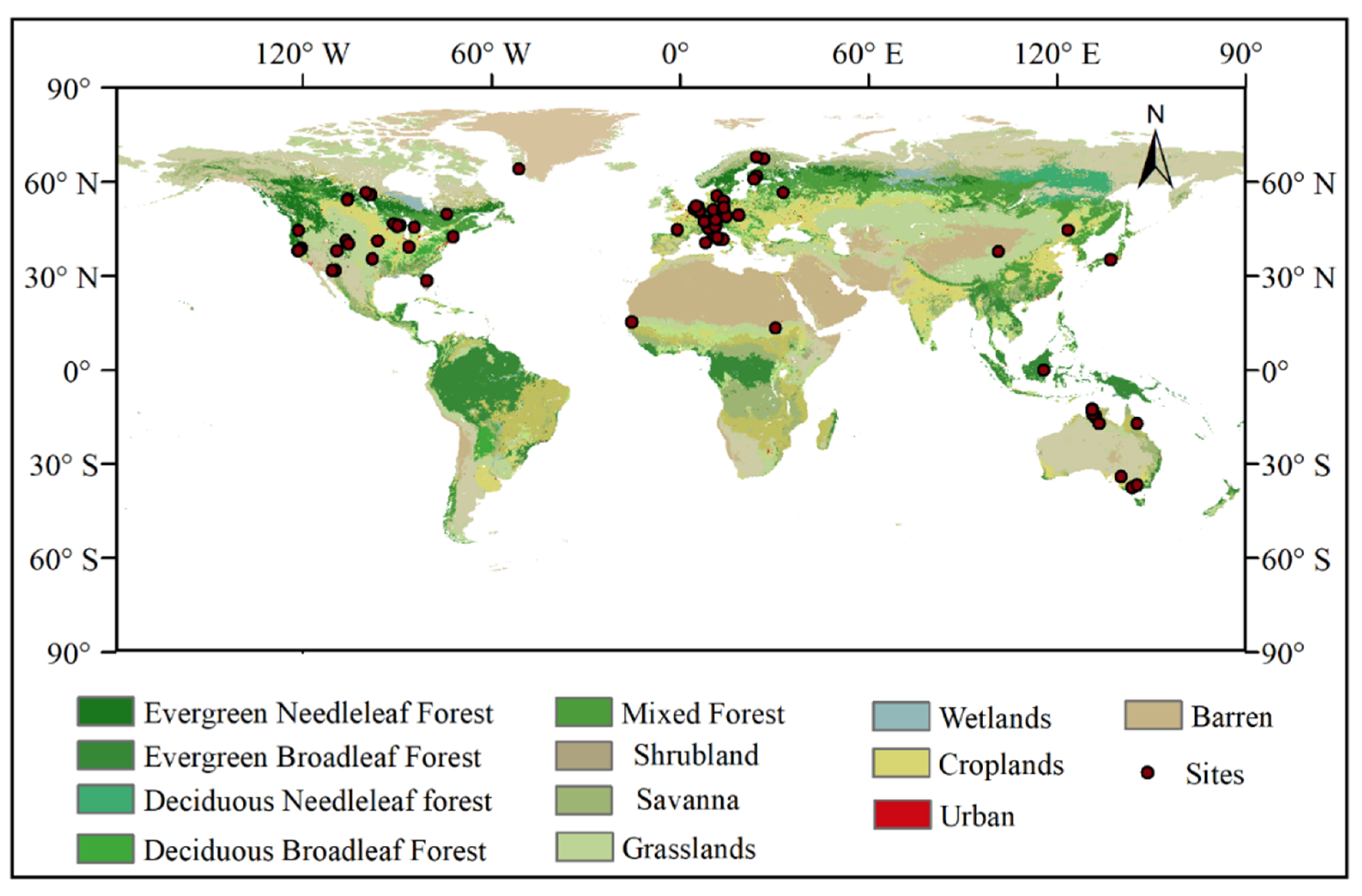
2.3. Eddy Covariance Measurements

The measurements of carbon, water, energy fluxes, and meteorological data were provided by The FLUXNET2015 dataset (https://fluxnet.org/data/fluxnet2015-dataset/,accessed on 29 Nov 2022) for more than 200 sites globally. These data were standardized by data processing, including quality control and gap-filling. The GPP data in this study (GPP_NT_VUT_REF) were partitioned from the net ecosystem exchange (NEE) dataset, following the nighttime partitioning approach. In the FLUXNET2015 dataset, sites were labeled with quality control flags ranging from 0 (poor quality) to 1 (good quality). We selected 78 Tier-1 sites with good quality for this study, encompassing ten terrestrial ecosystem vegetation types: deciduous broadleaf forest (DBF), evergreen broadleaf forest (EBF), evergreen needleleaf forest (ENF), mixed forest (MF), grasslands (GRA), savannas (SAV), shrubland (SHR), wetlands (WET), and cropland (C3/C4) (Figure 1). More detailed information about the sites is shown in Table S1 in the supplementary material. For each site, the FLUXNET2015 dataset was split into two parts, with data from the odd-numbered years used for the calibration model, and data from even-numbered years used for the validation model. For each variable, we aggregated the daily data into a 16-day time step to match the time step of the Landsat data.

2.4. Flux Footprint Modeling

The flux footprint prediction (FFP) model was used to compute the footprint of EC sites in this study. The FFP model is a dimensionalized parameterization of a backward Lagrangian stochastic dispersion model and was applied to a wide range of boundary layer stratifications and measurement heights. The input variables for the FFP model were: wind direction (WD), friction velocity (u_∗), wind speed (v), Obukhov length (L), instrument height (Z_m) and canopy height (h_c). The FFP model was able to provide results on size, position, and contour footprint climatology. More detailed information about footprint climatology calculation is available in [34]. The Obukhov length, canopy height, and instrument height were not directly provided in the FLUXNET2015 dataset. Obukhov length was therefore derived from a simple formula using the Monin–Obukhov similarity theory [35]. References for the canopy and instrument heights used here can be found in the references (Table S1).

The footprint calculations were conducted at half-hour time steps and aggregated to the 16-days resolution to generate two-dimensional contour lines of the footprint centered on the site. The footprints at the 80% contour of source weights were enough to truncate for analysis due to the extra 20% contour of footprints increasing with upwind distance from the receptor [20,36]. We estimated the flux footprint climatology with a grid size of 30 m spatial resolution at 16-day intervals to keep consistence with time step and spatial resolution from Landsat NDVI.

3. Results

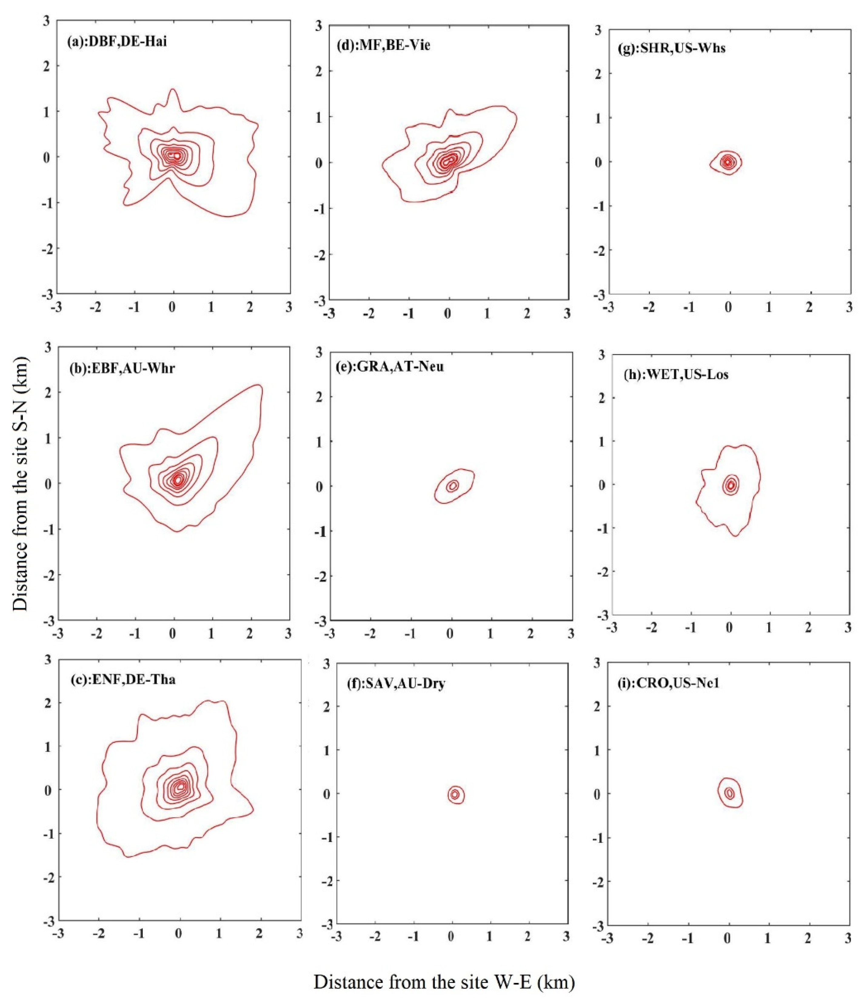
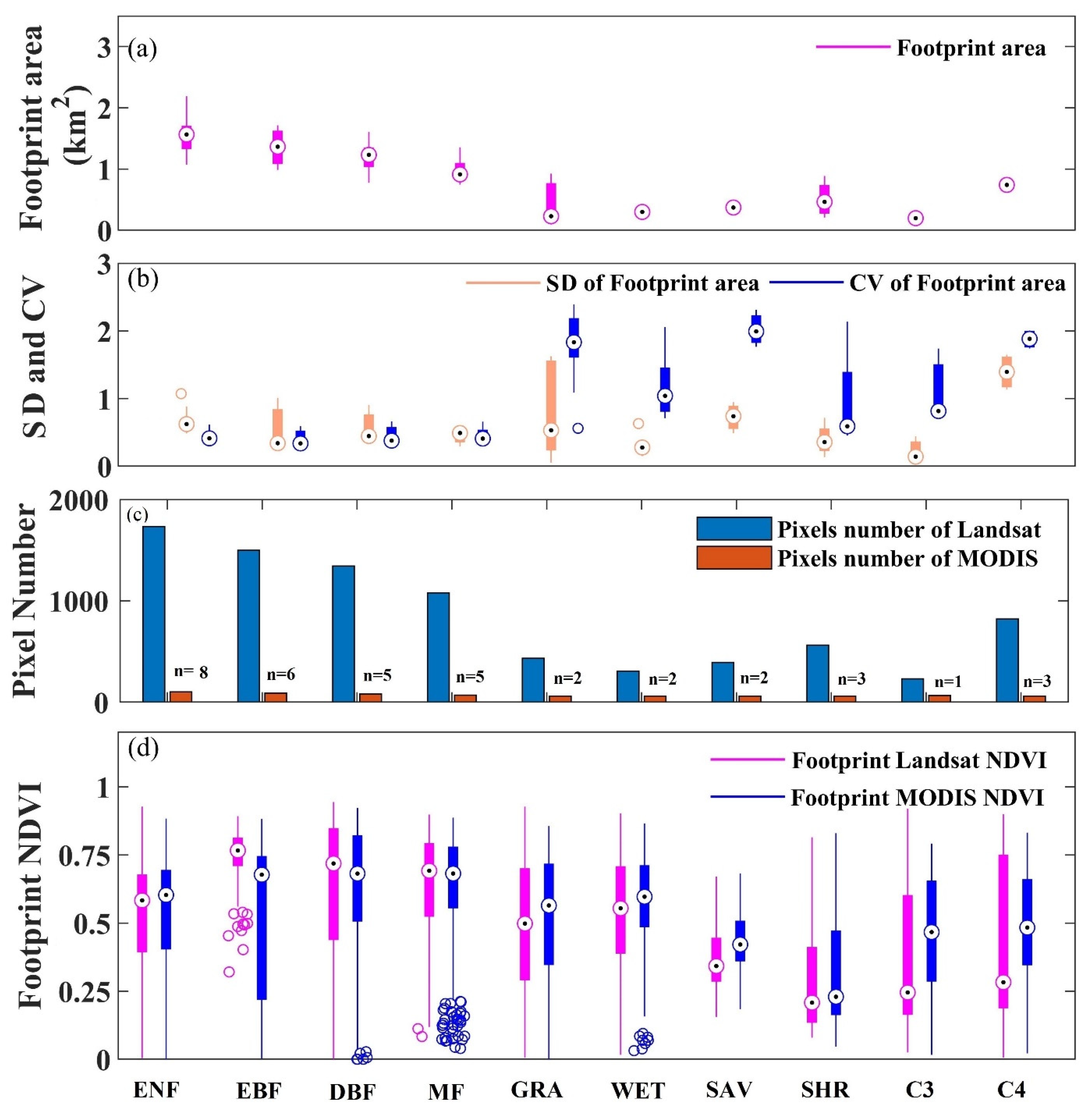
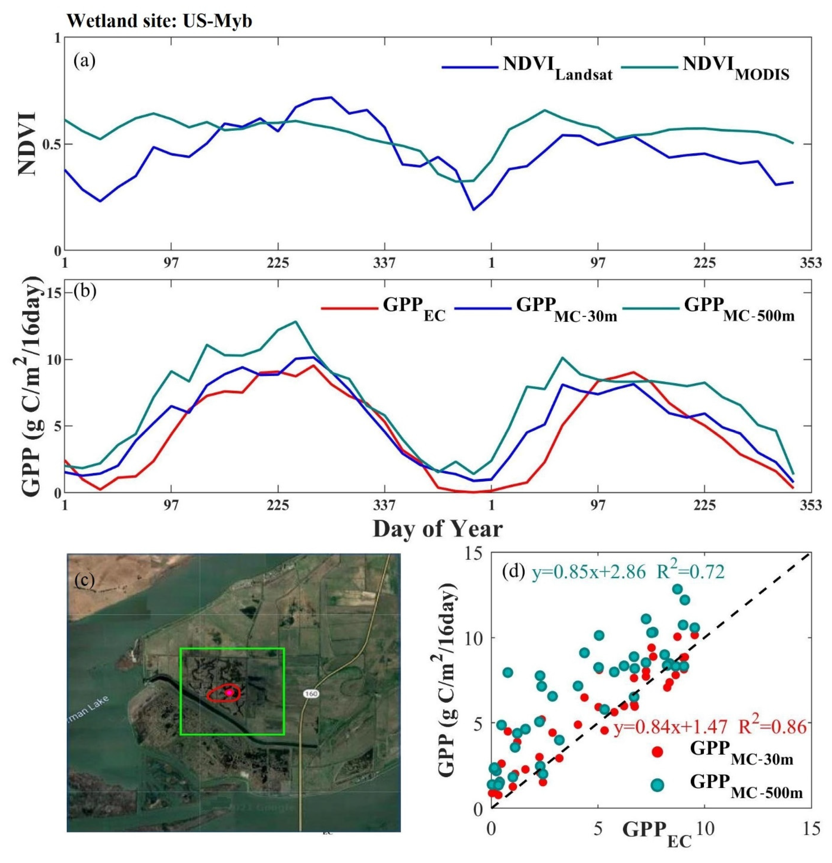
3.1. Heterogeneity of Flux Footprint

We calculated the footprint climatology for all 78 eddy covariance sites at 16-day time steps through the study period and considered the 80% contribution contour as each footprint’s climatology extents. The footprint climatology had a relative symmetric geometry and the size and position of the footprint climatology varied with wind directions, measurement height, and atmospheric stability. We selected ten sites, one representing each vegetation type, to show how footprint size varied across vegetation types (Figure 2). Overall, the footprint areas ranged from 0.09 km² to 2.18 km² at the 16-day scale among the 78 sites encompassing ten biomes. Evergreen broadleaf forests, evergreen needleleaf forests, deciduous broadleaf forests, and mixed forests had the largest footprint areas, ranging from 0.74 km² to 2.18 km², while footprint areas in grasslands, wetlands, savannas, shrublands and croplands were relatively small, covering around 0.13 km² to 0.82 km².

We examined the heterogeneity of the flux footprint and calculated the mean footprint area, SD, and CV of footprint area for each of the 78 flux sites at the 30 m spatial resolution over 16-day intervals. The mean footprint area of the 78 sites varied from 0.09 to 2.18 km² (Figure 3b). The SD and CV for footprint area are illustrated in Figure 3c and Figure 3d. Evergreen needleleaf forests, evergreen broadleaf forests, deciduous broadleaf forests, and mixed forests had a large mean footprint area with low SD and CV in footprint area. In contrast, grasslands, wetlands, savannas, and croplands had a relatively small mean footprint area with high SD and CV. For individual sites, grassland sites (e.g., IT-MBo, NL-Hor, US-ARc and US-ARb) and cropland sites (e.g., US-Ne1, US-Ne2 and US-Ne3) exhibited the largest SD among the 78 sites (Figure 3c and Figure 4b). This indicated that the heterogeneity of the FLUXNET footprint varied across the sites and vegetation types. This also suggested that the FLUXNET footprint was highly heterogeneous in grasslands, wetlands, savannas, and croplands.

To further examine how the footprint area and heterogeneity of flux footprint could be captured at 30 m and 500 m spatial resolution, we first calculated how many Landsat and MODIS pixels were needed to resolve each footprint area, and then computed the Landsat-footprint-NDVI and MODIS-footprint-NDVI. In general, the EC footprints were covered with only a few MODIS pixels, but needed thousands of Landsat pixels (Figure 4c). For example, the largest footprint areas were found for evergreen needle forests that covered 2.18 km². These were covered by a maximum of 8 MODIS 500 × 500 m pixels. They required 2422 of the much smaller (30 × 30 m) Landsat pixels to calculate NDVI. Cropland footprint areas with less than a 500 m radius were only covered by a single MODIS pixel, whereas there were 230 Landsat pixels available for calculating NDVI, enough to fully cover even this small footprint area. This demonstrated the huge difference in potential for spatial matches between the EC footprint and remote sensing pixels. The Landsat-footprint-NDVI was systematically higher than the MODIS-footprint-NDVI for forest ecosystems—but was less so for grasslands, wetlands, savannas, and croplands (Figure 4d). Moreover, the difference between the Landsat-footprint-NDVI and MODIS-footprint-NDVI was greatest for grasslands, wetlands, savannas, and croplands, and was lowest for forest ecosystems (Figure 4d).

3.2. Optimized Parameters

We used the MCMC method to estimate parameters for the revised EC-LUE model based on ground-GPP data. To examine the influence of the EC footprint on model accuracy at different spatial resolutions, we optimized the model parameters (ε_max, θ and VPD₀) separately, using Landsat-footprint NDVI and MODIS-footprint NDVI as driving factors. The model parameter calibrations used the same meteorological data, with a key difference; one used EC footprints derived from Landsat NDVI data at 30 m spatial resolution, and the other used EC footprints derived from MODIS NDVI data at 500 m spatial resolution. We generated two sets of optimized parameters for the revised EC-LUE model, both at 30 m spatial resolution (Landsat) and 500 m spatial resolution (MODIS), respectively. The 30-m optimized parameter values differed greatly from the 500-m optimized parameter values for grassland, wetland, savanna, shrubland, and cropland, but differed only slightly for forest ecosystems (

Table 1. The mean value and standard deviations of estimated parameters for revised EC-LUE model at 30 m spatial resolution (Landsat) and 500 m spatial resolution (MODIS).

Vegetation Type	Site Number	30 m Spatial Resolution			500 m Spatial Resolution
		εmax (g C/MJ)	θ (ppm)	VPD0 (k Pa)	εmax (g C/MJ)	θ (ppm)	VPD0 (k Pa)
EBF	3	3.67 ± 0.59	24.25 ± 7.72	0.33 ± 0.09	3.65 ± 0.59	25.27 ± 7.81	0.35 ± 0.09
DBF	12	2.97 ± 0.21	51.90 ± 6.72	1.59 ± 0.09	3.04 ± 0.23	51.05 ± 7.21	1.58 ± 0.09
ENF	21	2.97 ± 0.18	35.97 ± 3.26	1.08 ± 0.15	2.90 ± 0.19	31.93 ± 5.23	1.30 ± 0.17
MF	5	2.79 ± 0.21	43.31 ± 6.07	1.34 ± 0.12	2.83 ± 0.19	43.65 ± 5.45	1.34 ± 0.13
GRA	14	4.59 ± 0.06	64.72 ± 0.63	1.09 ± 0.01	4.44 ± 0.08	64.72 ± 0.75	1.09 ± 0.01
SAV	3	3.19 ± 0.30	25.39 ± 5.25	1.55 ± 0.15	2.60 ± 0.24	25.35 ± 5.29	1.56 ± 0.14
SHR	4	2.16 ± 0.33	57.59 ± 14.18	1.26 ± 0.23	2.02 ± 0.32	58.01 ± 14.23	1.24 ± 0.23
WET	9	3.10 ± 0.19	59.66 ± 5.15	1.40 ± 0.08	2.96 ± 0.18	59.71 ± 5.17	1.41 ± 0.07
C3 Crop	3	3.57 ± 0.29	60.55 ± 5.18	1.34 ± 0.18	3.27 ± 0.19	62.63 ± 4.75	1.37 ± 0.18
C4 Crop	4	4.81 ± 0.35	50.28 ± 5.74	1.52 ± 0.14	4.47 ± 0.30	51.12 ± 5.70	1.54 ± 0.15

). This reflected the difference between the Landsat-footprint NDVI and the MODIS-footprint NDVI.

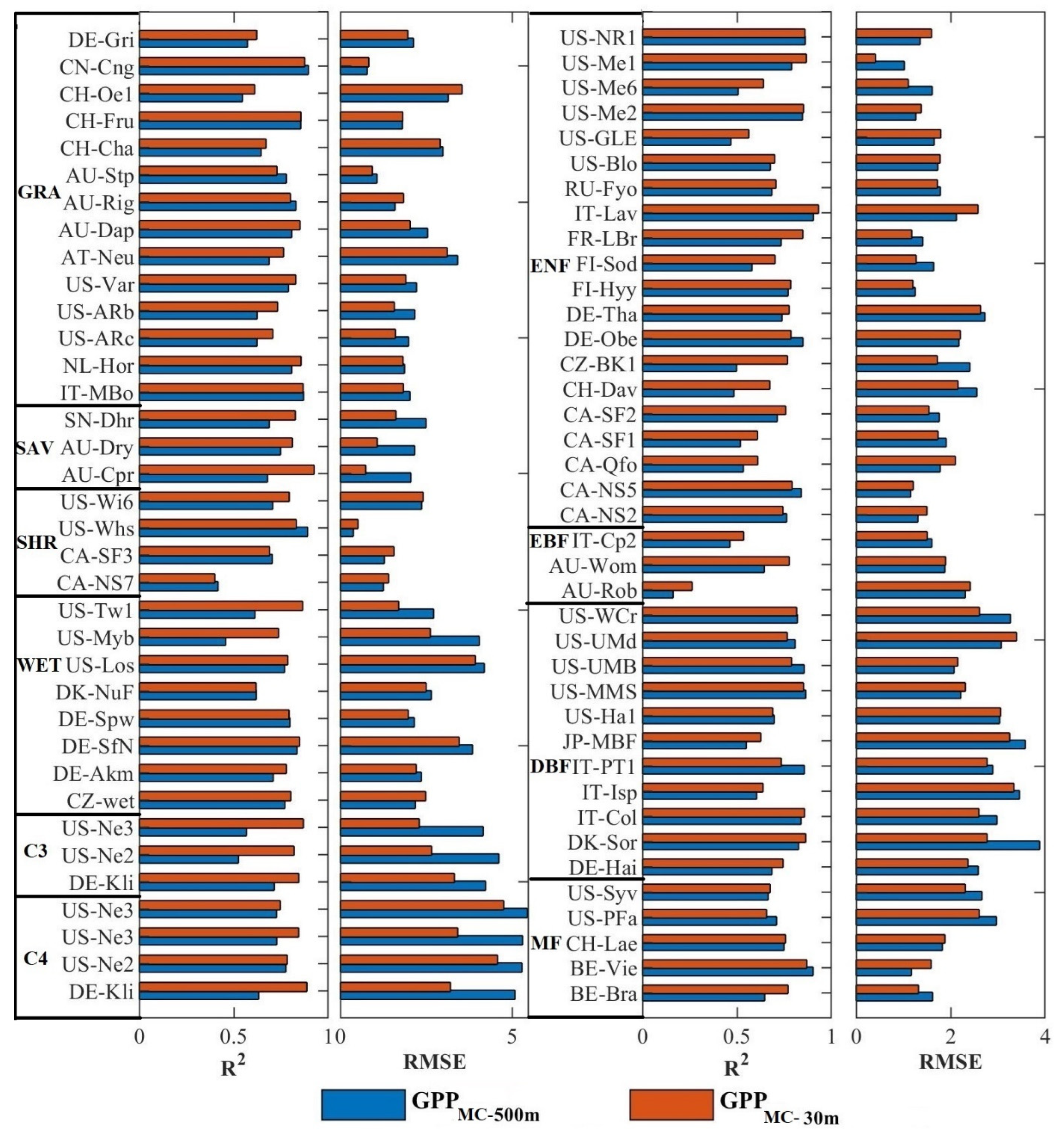
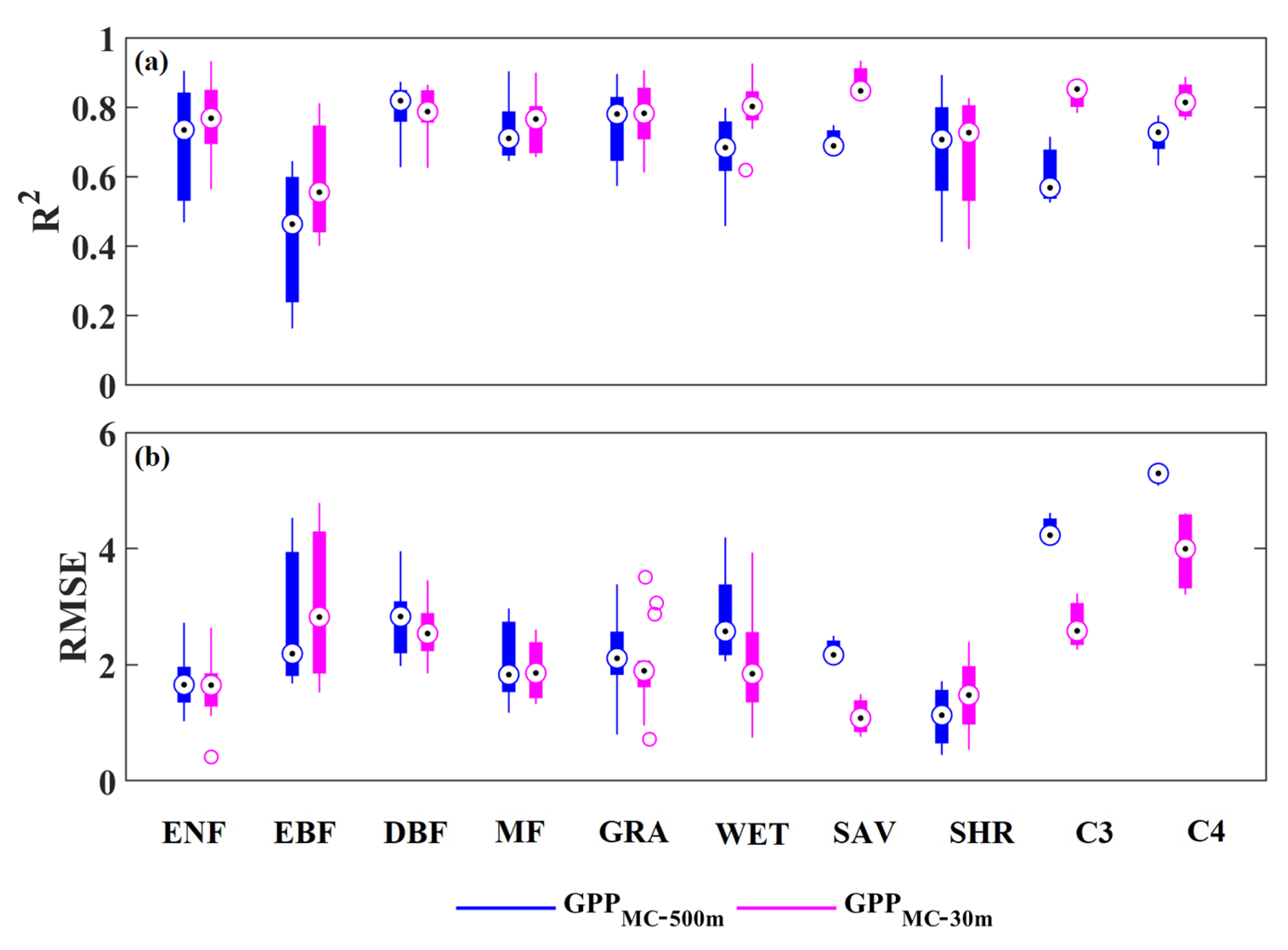
3.3. Model Accuracy Comparison

To examine the impact of spatial resolution of remote sensing pixels for EC footprints on modeling, we used our estimated parameters, optimized at 30 m and 500 m spatial resolution, respectively, pooled with corresponding Landsat-footprint-NDVI and MODIS-footprint-NDVI, to calculate GPP separately. The resulting GPP calculations were denoted GPP_MC-30m and GPP_MC-500m, respectively. The calculation of GPP_MC-30m and GPP_MC-500m used the same meteorological data (temperature, VPD, air atmospheric pressure, and CO₂ concentration) as driving data for fair comparison; the difference between GPP_MC-30m and GPP_MC-500m lay in the optimized parameters, Landsat-footprint-NDVI, and MODIS-footprint-NDVI.

We compared the accuracies of GPP_MC-30m and GPP_MC-500m at 16 days and calculated the R² and RMSE for each of 78 sites. On average, GPP_MC-30m and GPP_MC-500m explained 75% and 70% of the variance in site-based GPP across all 78 sites, respectively, indicating that the Landsat-footprint NDVI resulted in better GPP simulation performance than the MODIS-footprint NDVI (Figure 5). Compared with GPP_MC-500m, GPP_MC-30m exhibited higher R² values and lower RMSE values at most sites, particularly at the DE-Kli (R² = 0.88, RMSE = 3.21 g C/m²/16day), US-Ne2 (R² = 0.82, RMSE = 2.65 g C/m²/16day), and US-Ne3 (R² = 0.87, RMSE = 2.30 g C/m²/16day) cropland sites, at the US-Myb (R² = 0.73, RMSE = 2.62 g C/m²/16day) and US-Tw1 (R² = 0.86, RMSE = 1.70 g C/m²/16day) wetland sites, and at the AU-Cpr (R² = 0.92, RMSE = 0.74 g C/m²/16day) and SN-Dhr ( R² = 0.83, RMSE = 1.62 g C/m²/16day) savanna sites. Among the ten vegetation types, GPP_MC-30m explained significantly higher variance in tower GPP for C3, C4, WET, SAV, SHR, and EBF ecosystems than GPP_MC-500m, but with slightly higher variance in DBF, ENF, MF, and GRA ecosystems (Figure 6). For EBF ecosystems, compared with GPP_MC-500m, GPP_MC-30m still had slight improvement, with RMSE decreasing from 3.0 (g C/16 day) to 2.78 (g C/16 day) despite no improvement in terms of R² value (Figure 6).

We chose ten tower sites, representing ten vegetation types, to examine the seasonal cycles of simulated GPP and tower GPP. In general, compared with GPP_MC-500m, GPP_MC-30m was better able to capture the seasonal cycles of GPP at croplands site of US-Ne1 (Figure 7i), US-Ne3 (Figure 7j), and at the wetland site of US-Myb (Figure 7g). For example, we noted high surface spatial heterogeneity at cropland and wetland sites, such as the US-Ne1 and US-Myb sites (Figure 8c and Figure 9c). The NDVI derived from the Landsat and MODIS for the footprints at these two sites contained different phenological information, due to the different spatial scales at which the footprints were extracted (Figure 8a,c, Figure 9a,c). This meant that GPP_MC-30m was closer to the phenology of the site than GPP_MC-500m (Figure 8b and Figure 9b). Although the performance of both GPP_MC-30m and GPP_MC-500m exhibited overestimation in simulating GPP, the extent of the overestimates of the GPP_MC-30m was lower than that of GPP_MC-500m at the US-Ne1, US-Ne3, and US-Mby sites. GPP_MC-30m explained 87% and 86% of the variances of tower GPP at the US-Ne1 site and US-Myb site, respectively, while GPP_MC-500m explained only 58% and 72% of the variance at these sites, respectively (Figure 8d and Figure 9d). This indicated that the Landsat-footprint NDVI was more appropriate for simulating GPP for highly heterogeneous land surfaces than the MODIS-footprint NDVI. In 2005, there was a drought at AU-Dap, a grassland site in Australia, with high VPD and decreasing tower GPP. This was captured in GPP_MC-30m, which followed the tower data and decreased. However, there was no decrease in GPP_MC-500m (Figure 7f). This indicated that GPP_MC-30m could also capture variance in GPP introduced by drought at an individual site. For forest ecosystems (ENF, DBF, and MF), the performance of GPP_MC-30m in simulating GPP was comparable to GPP_MC-500m (Figure 7a–c).

To further assess the superiority of Landsat-footprint NDVI for simulating GPP for heterogeneous mountainous regions, we chose another five mountain sites, with steep surface gradients of over 10°, to evaluate the performance of GPP_MC-30m and GPP_MC-500m (

Table 2. Mountain site information and the value of R² and RMSE of the model performance at 30 m and 500 m resolution, respectively.

Sites Name	Long (°)	Lat (°)	Vegetation	Slope (°)	Elevation (m)	GPPMC-30 m		GPPMC-500 m
						R2	RMSE (g C/m2/16 Day)	R2	RMSE (g C/m2/16 Day)
AT-Neu	47.12	11.32	GRA	14.83	961–1307	0.76	3.11	0.69	3.42
CH-Lae	47.48	8.37	MF	21.44	489–846	0.76	1.87	0.75	1.82
JP-MBF	44.39	142.32	DBF	14.48	478–601	0.63	3.25	0.55	3.58
CZ-BK1	49.50	18.54	ENF	13.74	761–941	0.77	1.72	0.50	2.41
IT-Lav	45.96	11.28	ENF	12.10	1315–1466	0.93	2.58	0.90	2.12

). The comparison of model performances showed that GPP_MC-30m generally outperformed GPP_MC-500m, especially at JP-MBF and CZ-BK1 (Table 2), with a significant improvement for GPP estimation using Landsat-footprint NDVI, with R² increasing from 0.50 to 0.77, and RMSE decreasing from 2.41 to 1.72 g C/m²/16 day. This indicated that the smaller footprint of Landsat could greatly improve GPP estimation in areas with high heterogeneity.

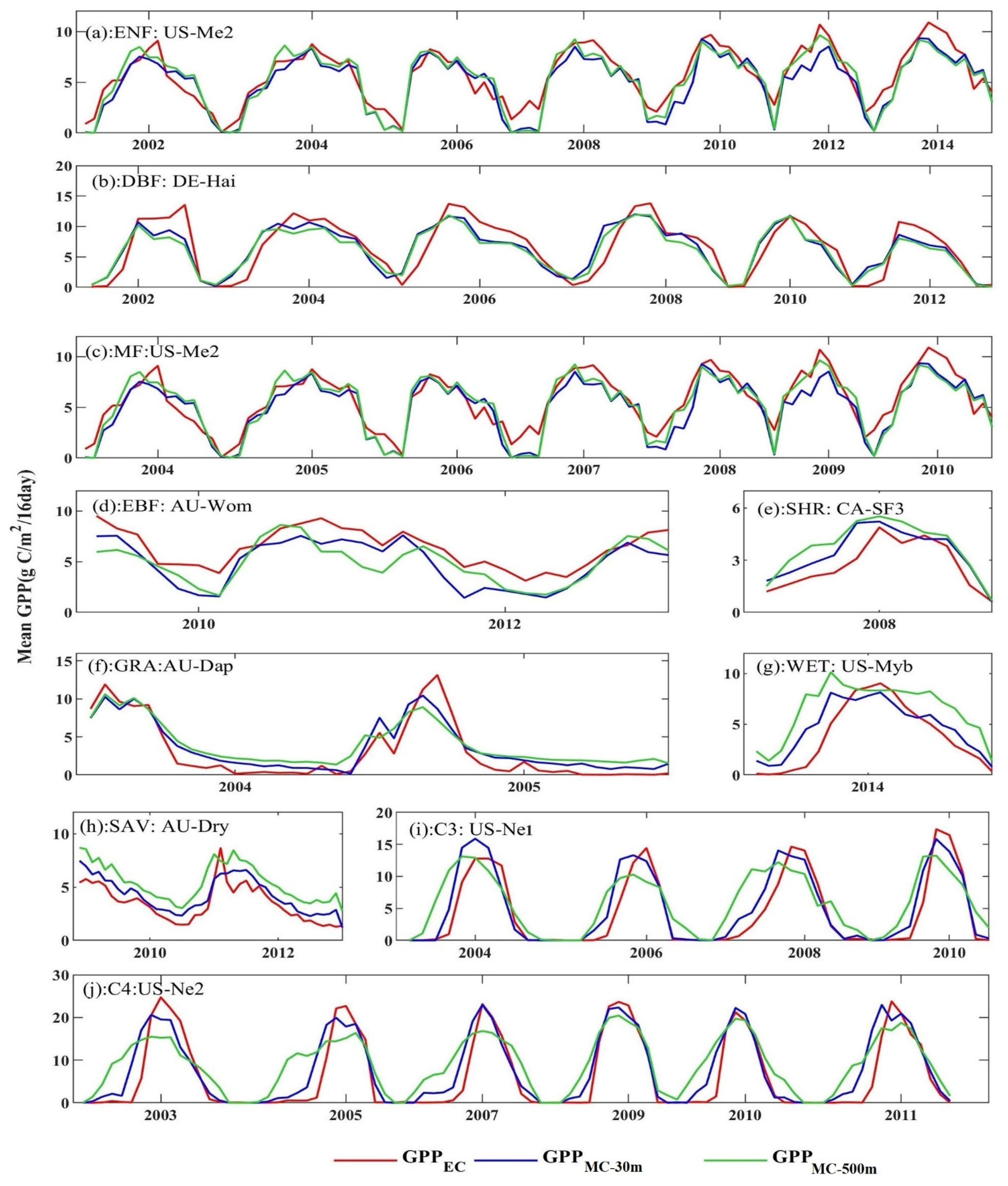
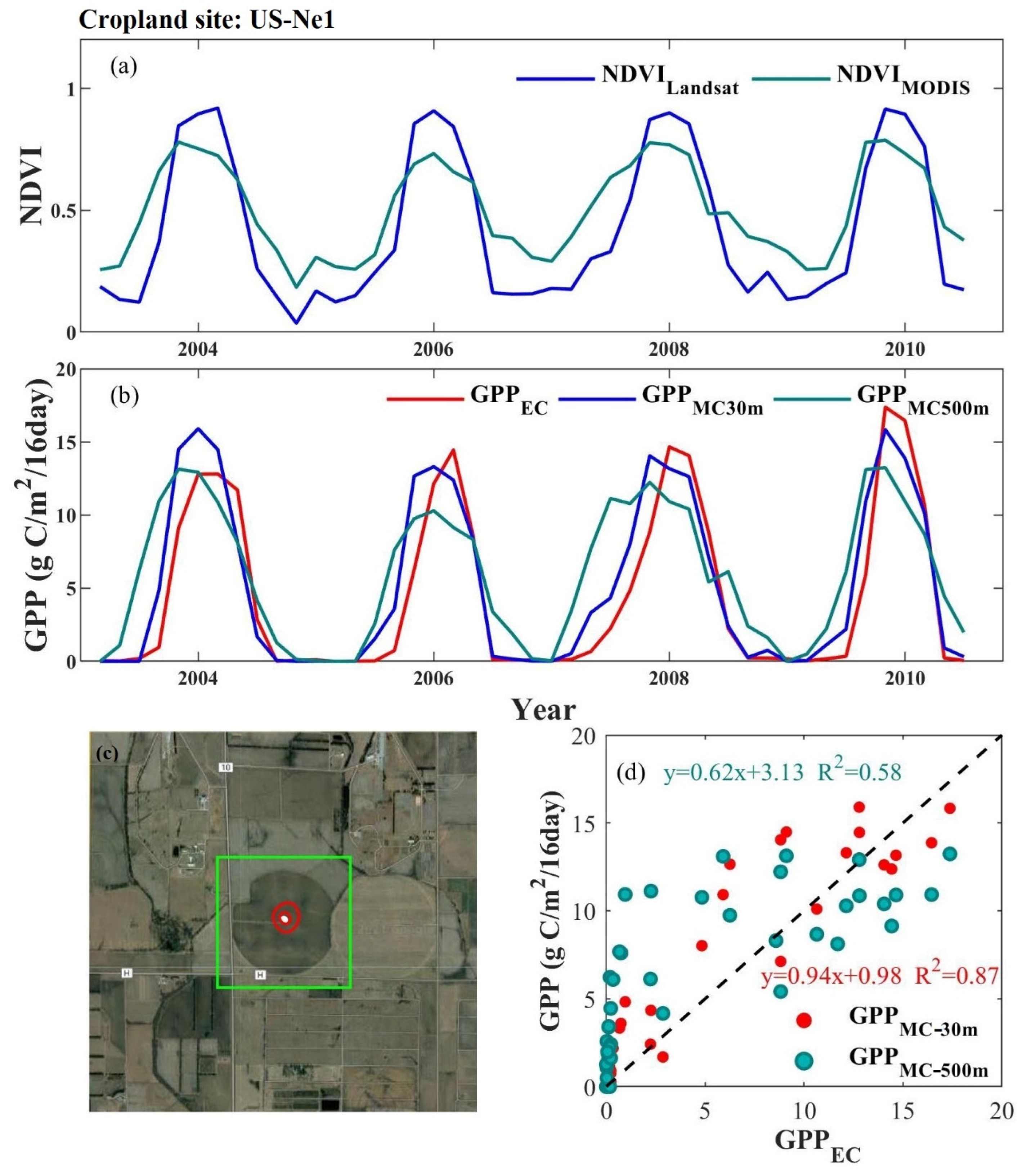
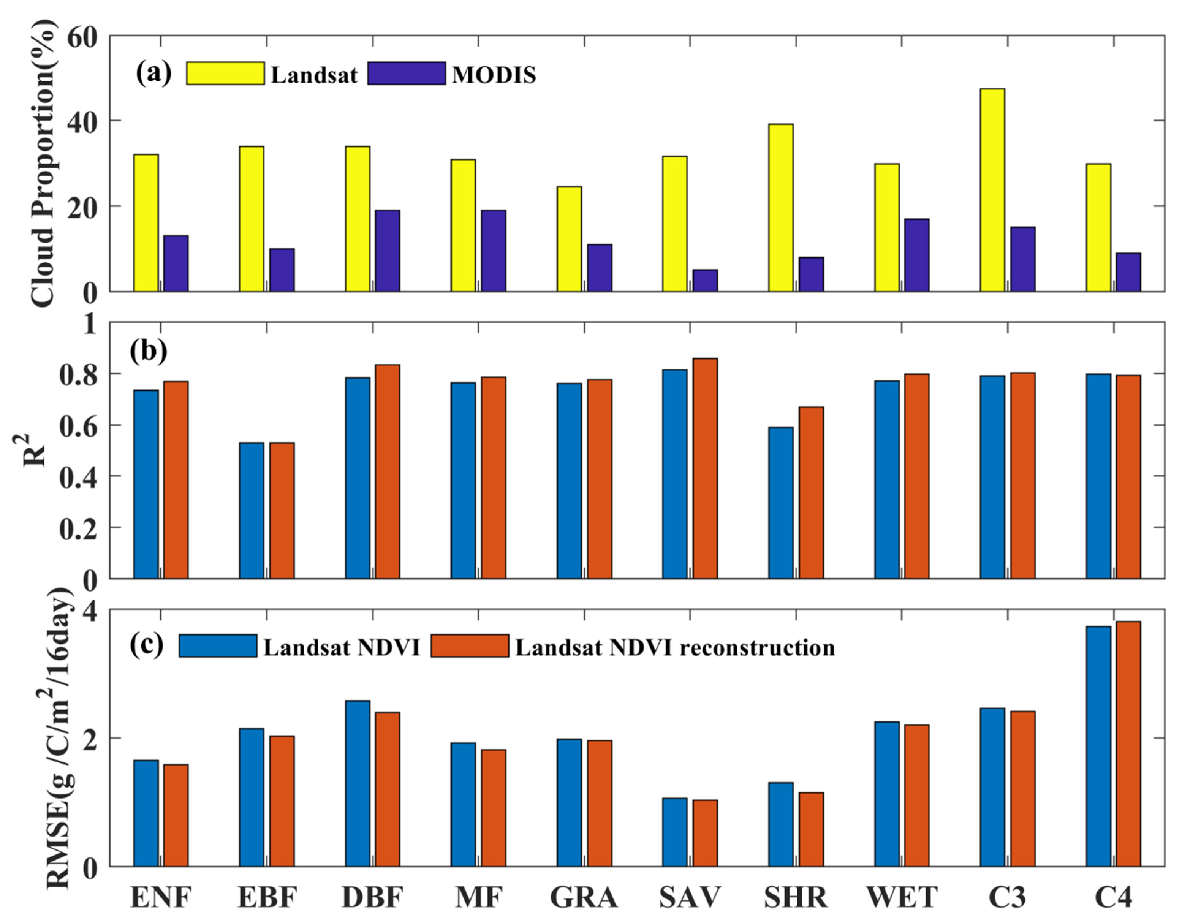
3.4. The Effect of Landsat Reconstruction on Model Accuracy

The Landsat-footprint NDVI was severely affected by cloud contamination, which accounted for 25~47% of the data that were acquired over the ten vegetation types (Figure 10a). In contrast, cloud contamination had a relatively small influence on the MODIS data, and only 5% to 19% were affected. The proportions of the Landsat-footprint NDVI data and the MODIS-footprint NDVI data that were affected by cloud at each site are illustrated in Figure 10. In this study, the missing Landsat-footprint NDVI data were not gapfilled or used for parameterization or evaluation of the model due to the serious data loss; the remaining Landsat-footprint NDVI was reconstructed. We compared the accuracy values of the model driven by the Landsat-footprint NDVI and reconstructed Landsat-footprint NDVI. For ENF, DBF, MF, GRA, SHR, and WET, the R² values were slightly higher and the RMSE values were slightly smaller when GPP was derived from the reconstructed Landsat-footprint NDVI than GPP driven by the Landsat-footprint NDVI (Figure 6). We found that the reconstruction of the Landsat-footprint NDVI resulted in a slight improvement in model performance at the ecosystem level, which indicated that the effect of the reconstruction on GPP estimation was small.

4. Discussion

In this study, we first optimized the parameters of the revised EC-LUE model using Landsat NDVI, spatially matched to the flux tower footprints at 30 m spatial resolution, and MODIS NDVI with a fixed footprint of 3 km × 3 km at 500 m spatial resolution. We then evaluated the performance of the model with our optimized parameters at different spatial scales. We found that matching the NDVI to the flux tower footprint significantly improved the GPP estimates at the 78 FLUXNET sites.

4.1. Impact of Spatial Scale Mismatch on Parameterization

Mismatches between the spatial scale of model parameters and input data can introduce significant uncertainties in GPP estimation [37]. In this study, we characterize how the footprint mismatching influenced the parameterization and performance of the revised EC-LUE model. We found that matching Landsat NDVI and flux footprints resulted in model parameters that were more representative at finer spatial resolutions, and considerably improved the estimated GPP, particularly for heterogeneous landscapes.

We considered that the footprint directly influenced estimated model parameters. This can be explained by the scale mismatch that existed between flux tower footprints and remote sensing data [14]. The tower-based observed GPP represented a flux integrated over the tower footprints, which had a typical area about 10³–10⁷ m². MODIS data has a resolution of 10⁶ m², and so a MODIS pixel is often several orders of magnitude larger than a tower footprint. The Landsat image with 30 m satellite-based grid cells was able to provide enough spatial information to capture the EC footprint and thus better reflect the boundary of the flux measurement [38]. This explained the difference that we found between the Landsat-footprint NDVI and MODIS-footprint NDVI (Figure 4d), which led to a difference in the estimated model parameters at 30 m and 500 m spatial resolution values (Table 1) and in the resulting GPP (Figure 5 and Figure 6).

To quantify the effects of the spatial resolution of the remote sensing data on the results of GPP estimation, we evaluated whether the footprint matching could still be effective for MODIS at 500 m spatial resolution rather than 30 m. We found that MODIS-footprint NDVI resulted in poor estimates of GPP for grasslands, wetlands, savannas, shrublands, and croplands due to the low proportion of footprint area within a MODIS pixel of a high heterogeneous surface. Landsat-footprint-NDVI consistently had a robust and reliable performance in estimation of GPP at ten vegetation types. This highlighted the advantage of high spatial resolution remote sensing data when considering the footprint for GPP simulation; these data could not be replaced by coarse spatial resolution remote sensing data.

The differences between the optimized parameters and the performance of the resulting models varied only slightly at forest ecosystem sites, but were large for other ecosystem types, which was related to vegetation heterogeneity and footprint size. For homogeneous vegetation, such as a forest ecosystem with a relatively large footprint, the fixed areas of 3 km × 3 km surrounding the towers for MODIS-footprint-NDVI could adequately represent the footprint of flux measurement. However, this was not true for other ecosystems with more heterogeneous vegetation, such as savanna and cropland, where the flux measurement footprints were smaller. Therefore, the impact of spatial mismatch between satellite imagery and EC footprints was more acute in heterogeneous landscapes or complex terrains [39,40], which led to the large variance of parameters and GPP estimation, especially in grasslands, wetlands, savannas, shrublands, and croplands (Figure 6).

4.2. To What Degree Do Landsat Images Improve GPP Estimation

The improvement in GPP estimation that was achieved by using fine-resolution Landsat data, compared to relatively coarse-resolution MODIS data, varied between sites, vegetation types, and for different surface heterogeneities. At the site level, model accuracy improved by 1~29% over the 78 sites when Landsat-footprint NDVI data were used to drive the model rather than MODIS-footprint NDVI data (Figure 5). For vegetation types, using Landsat-footprint NDVI data improved GPP estimates by 18% for savannas, 14% for croplands, and 9% for wetlands; Landsat-footprint NDVI was comparable to or slightly stronger than MODIS-footprint NDVI in estimation GPP at grasslands, shrublands, and forest ecosystems (Figure 6). Additionally, the accuracy of GPP estimates improved dramatically at sites with high surface heterogeneity when Landsat-footprint NDVI data were used. For example, R² increased by 0.29 at the US-Ne1 cropland site with (Figure 8), by 0.14 at the US-Myb wetland site (Figure 9), and by 27% at the CZ-BK1 mountain (Table 2). This showed that Landsat-footprint-NDVI can be used to describe the spatial surface heterogeneity of mixed planting in cropland, grass and water in wetlands, and complex terrain, providing more detailed phenological information to better describe GPP distribution.

Surface heterogeneity fell into two general categories in this study. The first was the mountainous regions. Characteristics of these regions included vegetation heterogeneity and surface topography with steep slopes and elevation variance, which were important factors for the GPP estimation. Vegetation heterogeneity directly determines photosynthetic capacity and topography influences the redistribution of precipitation and incoming solar radiation [41]. Moreover, vegetation is often highly fragmented in these regions due to the vegetation structures with climatic and topographic gradients [42]. Therefore, the high spatial heterogeneity of mountain vegetation could influence the quality of MODIS NDVI at coarse resolution. Additionally, data from the higher spatial resolution Landsat sensor could provide more detailed information for mountainous regions, despite topographic illumination condition correction being of no consideration [43]. Moreover, the authors of [44] suggested that considering the footprint of flux towers in mountainous regions could also improve GPP estimates. Our results revealed that remote sensing data with high spatial resolution, combined with introducing the footprint into model parametrization, improved GPP estimates in mountainous areas with strong heterogeneity (Table 2). This was because high resolution remote sensing data provided sufficient spatial information to capture surface heterogeneity [38].

The second category of surface heterogeneity in this study was landscape fragmentation in croplands and wetlands, which have high surface heterogeneity and relatively small footprints. Using MODIS NDVI as the forcing data for model GPP simulation may not have accurately captured the phenology of the plant with a strong spring green-up signal at the US-Ne1 [45] and US-Myb sites. Similar to the problems associated with using a coarse data source for mountainous regions, MODIS NDVI with coarse resolution contained other plant information due to fragmentation planting within the footprint area. Furthermore, the mismatch of spatial resolution of MODIS NDVI and EC footprint resulted in mixed pixel information, which led to the MODIS NDVI being unable to capture the phenology information of plants within the footprint area (Figure 8 and Figure 9). However, Landsat images, with their high spatial resolution, had an absolute advantage in capturing the pixels representing the flux footprint [24]. The large difference between the spatial resolutions of Landsat and MODIS led to differences in their ability to capture the footprints at heterogeneous sites, which led to GPP_MC-30m outperforming GPP_MC-500m for ecosystems with a fragmented plant structure (Figure 8 and Figure 9).

4.3. Limitations and Perspectives

Landsat NDVI has a higher spatial resolution than MODIS NDVI and is less affected by spatial compositing and mixed pixels, making it better suited to capturing surface details and for characterizing flux tower footprints [46]. However, the 16-day revisit cycle and problems with frequent cloud contamination and snow limit the amount of Landsat data, and therefore Landsat available data are often insufficient for research on vegetation seasonal variability [47,48]. Although gap-filling and reconstruction are widely used methods for improving the quality of Landsat data, the effects of gap-filling and reconstruction on the Landsat data were small for GPP estimates [15,49].

It is often more appropriate to use MODIS NDVI than Landsat NDVI data, despite the coarser resolution of the former, owing to its high revisit frequency and low cloud proportion of cloud-affected pixels [50]. In the future, blending high spatial resolution data (i.e., Landsat) with high temporal resolution (i.e., MODIS) could provide an alternative data source with high temporal resolution and high spatial resolution that would be better able to capture spatiotemporal patterns in ecosystem dynamics [51]. If combined with higher temporal-resolution data in this way, the 30-m resolution Landsat NDVI could be used to simulate GPP at regional or global scales. The advantage of using remote sensing data with high resolution when simulating GPP for heterogeneous landscapes is the superiority of the resulting general GPP monitoring at medium or coarse resolution—which could then capture more detailed GPP dynamics and responses to heterogeneous landscape changes such as cropland agriculture, land use change, and human activities.

5. Conclusions

We utilized the FFP model to evaluate the footprints of the 78 FLUXNET sites across ten vegetation types on the globe and calculated the Landsat-footprint NDVI and the MODIS-footprint NDVI. We optimized the parameters (ε_max, θ and VPD₀) of the revised EC-LUE model and compared the model performance using Landsat-footprint NDVI, incorporating spatial and temporal dynamics of the flux footprint at 30 m spatial resolution and MODIS-footprint NDVI with a fixed footprint at 500 m spatial resolution. Our results showed that Landsat-footprint NDVI, compared with MODIS NDVI, could improve GPP estimation by 18% for savannas, 14% for croplands, 9% for wetlands, and 6% for evergreen needleleaf forest, with slight improvement or comparable performance as compared to other ecosystems. This indicated that using NDVI with high spatial resolution resulted in more detailed GPP estimates, particularly for areas with heterogeneous surfaces. Our study highlighted the significance of using data with a high spatial resolution to match the flux tower footprint more accurately and improve estimation of GPP.

References

1. Xiao, J.; Chevallier, F.; Gomez, C.; Guanter, L.; Hicke, J.A.; Huete, A.R.; Ichii, K.; Ni, W.; Pang, Y.; Rahman, A.F.; et al. Remote sensing of the terrestrial carbon cycle: A review of advances over 50 years. Remote Sens. Environ. 2019, 233, 111383. [Google Scholar] [CrossRef]
2. Yuan, W.; Piao, S.; Qin, D.; Dong, W.; Xia, J.; Lin, H.; Chen, M. Influence of Vegetation Growth on the Enhanced Seasonality of Atmospheric CO2. Global Biogeochem. Cycles 2018, 32, 32–41. [Google Scholar] [CrossRef]
3. Dong, J.; Fu, Y.; Wang, J.; Tian, H.; Fu, S.; Niu, Z.; Han, W.; Zheng, Y.; Huang, J.; Yuan, W. Early-season mapping of winter wheat in China based on Landsat and Sentinel images. Earth Syst. Sci. Data 2020, 12, 3081–3095. [Google Scholar] [CrossRef]
4. Huang, X.; Xiao, J.; Ma, M. Evaluating the Performance of Satellite-Derived Vegetation Indices for Estimating Gross Primary Productivity Using FLUXNET Observations across the Globe. Remote Sens. 2019, 11, 1823. [Google Scholar] [CrossRef] [Green Version]
5. Xiao, X.M.; Zhang, Q.Y.; Braswell, B.; Urbanski, S.; Boles, S.; Wofsy, S.; Berrien, M.; Ojima, D. Modeling gross primary production of temperate deciduous broadleaf forest using satellite images and climate data. Remote Sens. Environ. 2004, 91, 256–270. [Google Scholar] [CrossRef]
6. Running, S.W.; Nemani, R.R.; Heinsch, F.A.; Zhao, M.; Reeves, M.; Hashimoto, H. A continuous satellite-derived measure of global terrestrial primary production. Bioscience 2004, 54, 547–560. [Google Scholar] [CrossRef]
7. Yuan, W.P.; Liu, S.; Zhou, G.S.; Zhou, G.Y.; Tieszen, L.L.; Baldocchi, D.; Bernhofer, C.; Gholz, H.; Goldstein, A.H.; Goulden, M.L.; et al. Deriving a light use efficiency model from eddy covariance flux data for predicting daily gross primary production across biomes. Agric. For. Meteorol. 2007, 143, 189–207. [Google Scholar] [CrossRef] [Green Version]
8. Yuan, W.; Zheng, Y.; Piao, S.; Ciais, P.; Lombardozzi, D.; Wang, Y.; Ryu, Y.; Chen, G.; Dong, W.; Hu, Z.; et al. Increased atmospheric vapor pressure deficit reduces global vegetation growth. Sci. Adv. 2019, 5, 1–13. [Google Scholar] [CrossRef] [Green Version]
9. Farquhar, A.G.D.; Von Caemmerer, S.; Berry, J.A. A biochemical model of photosynthetic CO2 assimilation in leaves of C3 species. Planta 1980, 149, 78–90. [Google Scholar] [CrossRef] [Green Version]
10. Friend, A.D.; Arneth, A.; Kiang, N.Y.; Lomas, M.; Ogée, J.; Rödenbeck, C.; Running, S.W.; Santaren, J.D.; Sitch, S.; Viovy, N.; et al. FLUXNET and modelling the global carbon cycle. Glob. Chang. Biol. 2007, 13, 610–633. [Google Scholar] [CrossRef]
11. Running, S.W.; Thornton, P.E.; Nemani, R.; Glassy, J.M. Global Terrestrial Gross and Net Primary Productivity from the Earth Observing System. In Methods in Ecosystem Science; Springer: New York, NY, USA, 2000; pp. 44–57. [Google Scholar]
12. Zhang, Y.; Xiao, X.; Wu, X.; Zhou, S.; Zhang, G.; Qin, Y.; Dong, J. A global moderate resolution dataset of gross primary production of vegetation for 2000-2016. Sci. Data 2017, 4, 170165. [Google Scholar] [CrossRef] [Green Version]
13. Zheng, Y.; Shen, R.; Wang, Y.; Li, X.; Liu, S.; Liang, S.; Chen, J.M.; Ju, W.; Zhang, L.; Yuan, W. Improved estimate of global gross primary production for reproducing its long-Term variation, 1982-2017. Earth Syst. Sci. Data 2020, 12, 2725–2746. [Google Scholar] [CrossRef]
14. Huang, X.; Zheng, Y.; Zhang, H.; Lin, S.; Liang, S.; Li, X.; Ma, M.; Yuan, W. High spatial resolution vegetation gross primary production product: Algorithm and validation. Sci. Remote Sens. 2022, 5, 100049. [Google Scholar] [CrossRef]
15. Lin, S.; Huang, X.; Zheng, Y.; Zhang, X.; Yuan, W. An Open Data Approach for Estimating Vegetation Gross Primary Production at Fine Spatial Resolution. Remote Sens. 2022, 14. [Google Scholar] [CrossRef]
16. Hansen, M.C.; Potapov, P.V.; Moore, R.; Hancher, M.; Turubanova, S.A.; Tyukavina, A.; Thau, D.; Stehman, S.V.; Goetz, S.J.; Loveland, T.R.; et al. High-Resolution Global Maps of 21st-Century Forest Cover Change. Science 2013 342, 850–853. [CrossRef] [Green Version]
17. Parazoo, N.C.; Coleman, R.W.; Yadav, V.; Stavros, E.N.; Hulley, G.; Hutyra, L. Diverse biosphere influence on carbon and heat in mixed urban Mediterranean landscape revealed by high resolution thermal and optical remote sensing. Sci. Total Environ. 2022, 806, 151335. [Google Scholar] [CrossRef]
18. Dong, J.; Lu, H.; Wang, Y.; Ye, T.; Yuan, W. Estimating winter wheat yield based on a light use efficiency model and wheat variety data. ISPRS J. Photogramm. Remote Sens. 2020, 160, 18–32. [Google Scholar] [CrossRef]
19. Robinson, N.P.; Allred, B.W.; Smith, W.K.; Jones, M.O.; Moreno, A.; Erickson, T.A.; Naugle, D.E.; Running, S.W. Terrestrial primary production for the conterminous United States derived from Landsat 30 m and MODIS 250 m. Remote Sens. Ecol. Conserv. 2018, 4, 264–280. [Google Scholar] [CrossRef]
20. Chu, H.; Luo, X.; Ouyang, Z.; Chan, W.S.; Dengel, S.; Biraud, S.C.; Torn, M.S.; Metzger, S.; Kumar, J.; Arain, M.A.; et al. Representativeness of Eddy-Covariance flux footprints for areas surrounding AmeriFlux sites. Agric. For. Meteorol. 2021, 301–302, 108350. [Google Scholar] [CrossRef]
21. Chen, B.; Coops, N.C.; Fu, D.; Margolis, H.A.; Amiro, B.D.; Black, T.A.; Arain, M.A.; Barr, A.G.; Bourque, C.P.-A.; Flanagan, L.B.; et al. Characterizing spatial representativeness of flux tower eddy-covariance measurements across the Canadian Carbon Program Network using remote sensing and footprint analysis. Remote Sens. Environ. 2012, 124, 742–755. [Google Scholar] [CrossRef]
22. Verma, M.; Friedl, M.A.; Law, B.E.; Bonal, D.; Kiely, G.; Black, T.A.; Wohlfahrt, G.; Moors, E.J.; Montagnani, L.; Marcolla, B.; et al. Improving the performance of remote sensing models for capturing intra- and inter-annual variations in daily GPP: An analysis using global FLUXNET tower data. Agric. For. Meteorol. 2015, 214–215, 416–429. [Google Scholar] [CrossRef] [Green Version]
23. Stockli, R.; Rutishauser, T.; Dragoni, D.; O’Keefe, J.; Thornton, P.E.; Jolly, M.; Lu, L.; Denning, A.S. Remote sensing data assimilation for a prognostic phenology model. J. Geophys. Res. 2008, 113, G04021. [Google Scholar] [CrossRef]
24. Wagle, P.; Gowda, P.H.; Neel, J.P.S.; Northup, B.K.; Zhou, Y. Integrating eddy fl uxes and remote sensing products in a rotational grazing native tallgrass prairie pasture. Sci. Total Environ. 2020, 712, 136407. [Google Scholar] [CrossRef] [PubMed]
25. Gitelson, A.A.; Peng, Y.; Masek, J.G.; Rundquist, D.C.; Verma, S.; Suyker, A.; Baker, J.M.; Hatfield, J.L.; Meyers, T. Remote estimation of crop gross primary production with Landsat data. Remote Sens. Environ. 2012, 121, 404–414. [Google Scholar] [CrossRef] [Green Version]
26. Knox, S.H.; Dronova, I.; Sturtevant, C.; Oikawa, P.Y.; Matthes, J.H.; Verfaillie, J.; Baldocchi, D. Using digital camera and Landsat imagery with eddy covariance data to model gross primary production in restored wetlands. Agric. For. Meteorol. 2017, 237–238, 233–245. [Google Scholar] [CrossRef] [Green Version]
27. Yuan, W.P.; Liu, S.G.; Yu, G.R.; Bonnefond, J.M.; Chen, J.Q.; Davis, K.; Desai, A.R.; Goldstein, A.H.; Gianelle, D.; Rossi, F.; et al. Global estimates of evapotranspiration and gross primary production based on MODIS and global meteorology data. Remote Sens. Environ. 2010, 114, 1416–1431. [Google Scholar] [CrossRef] [Green Version]
28. Huang, X.; Xiao, J.; Wang, X.; Ma, M. Improving the global MODIS GPP model by optimizing parameters with FLUXNET data. Agric. For. Meteorol. 2021, 300, 108314. [Google Scholar] [CrossRef]
29. Zhang, Y.; Kong, D.; Gan, R.; Chiew, F.H.S.; McVicar, T.R.; Zhang, Q.; Yang, Y. Coupled estimation of 500 m and 8-day resolution global evapotranspiration and gross primary production in 2002–2017. Remote Sens. Environ. 2019, 222, 165–182. [Google Scholar] [CrossRef]
30. Eilers, P.H.C. A Perfect Smoother. Anal. Chem. 2003, 75, 3631–3636. [Google Scholar] [CrossRef]
31. Atzberger, C.; Eilers, P.H.C. A time series for monitoring vegetation activity and phenology at 10-daily time steps covering large parts of South America. Int. J. Digit. Earth 2011, 4, 365–386. [Google Scholar] [CrossRef]
32. Frasso, G.; Eilers, P.H.C. L- and V-curves for optimal smoothing. Stat. Modelling 2015, 15, 91–111. [Google Scholar] [CrossRef]
33. Kong, D.; Zhang, Y.; Gu, X.; Wang, D. A robust method for reconstructing global MODIS EVI time series on the Google Earth Engine. ISPRS J. Photogramm. Remote Sens. 2019, 155, 13–24. [Google Scholar] [CrossRef]
34. Kljun, N.; Calanca, P.; Rotach, M.W.; Schmid, H.P. A simple two-dimensional parameterisation for Flux Footprint Prediction (FFP). Geosci. Model Dev. 2015, 8, 3695–3713. [Google Scholar] [CrossRef] [Green Version]
35. Grimmond, C.S.B.; Cleugh, H.A. A simple method to determine Obukhov lengths for suburban areas. J. Appl. Meteorol. 1994, 33, 435–440. [Google Scholar] [CrossRef]
36. Kim, J.; Hwang, T.; Schaaf, C.L.; Kljun, N.; Munger, J.W. Seasonal variation of source contributions to eddy-covariance CO2 measurements in a mixed hardwood-conifer forest. Agric. For. Meteorol. 2018, 253–254, 71–83. [Google Scholar] [CrossRef]
37. Pei, Y.; Dong, J.; Zhang, Y.; Yuan, W.; Doughty, R.; Yang, J. Evolution of light use efficiency models: Improvement, uncertainties, and implications. Agric. For. Meteorol. 2022, 317, 108905. [Google Scholar] [CrossRef]
38. Zhou, Y.; Xiao, X.; Wagle, P.; Bajgain, R.; Mahan, H.; Basara, J.B.; Dong, J.; Qin, Y.; Zhang, G.; Luo, Y.; et al. Examining the short-term impacts of diverse management practices on plant phenology and carbon fluxes of Old World bluestems pasture. Agric. For. Meteorol. 2017, 237–238, 60–70. [Google Scholar] [CrossRef] [Green Version]
39. Gelybó, G.; Barcza, Z.; Kern, A.; Kljun, N. Effect of spatial heterogeneity on the validation of remote sensing based GPP estimations. Agric. For. Meteorol. 2013, 174–175, 43–53. [Google Scholar] [CrossRef]
40. Giannico, V.; Chen, J.; Shao, C.; Ouyang, Z.; John, R.; Lafortezza, R. Contributions of landscape heterogeneity within the footprint of eddy-covariance towers to flux measurements. Agric. For. Meteorol. 2018, 260, 144–153. [Google Scholar] [CrossRef]
41. Xie, X.; Li, A.; Jin, H.; Yin, G.; Bian, J. Spatial downscaling of gross primary productivity using topographic and vegetation heterogeneity information: A case study in the Gongga Mountain region of China. Remote Sens. 2018, 10, 647. [Google Scholar] [CrossRef]
42. Jin, H.; Li, A.; Bian, J.; Nan, X.; Zhao, W.; Zhang, Z.; Yin, G. Intercomparison and validation of MODIS and GLASS leaf area index (LAI) products over mountain areas: A case study in southwestern China. Int. J. Appl. Earth Obs. Geoinf. 2017, 55, 52–67. [Google Scholar] [CrossRef]
43. Young, N.E.; Anderson, R.S.; Chignell, S.M.; Vorster, A.G.; Lawrence, R.; Evangelista, P.H. A survival guide to Landsat preprocessing. Ecology 2017, 98, 920–932. [Google Scholar] [CrossRef] [PubMed] [Green Version]
44. Xie, X.; Chen, J.M.; Gong, P.; Li, A. Spatial Scaling of Gross Primary Productivity Over Sixteen Mountainous Watersheds Using Vegetation Heterogeneity and Surface Topography. J. Geophys. Res. Biogeosciences 2021, 126, 1–21. [Google Scholar] [CrossRef]
45. Yuan, W.; Cai, W.; Nguy-Robertson, A.L.; Fang, H.; Suyker, A.E.; Chen, Y.; Dong, W.; Liu, S.; Zhang, H. Uncertainty in simulating gross primary production of cropland ecosystem from satellite-based models. Agric. For. Meteorol. 2015, 207, 48–57. [Google Scholar] [CrossRef] [Green Version]
46. Beck, H.E.; McVicar, T.R.; van Dijk, A.I.J.M.; Schellekens, J.; de Jeu, R.A.M.; Bruijnzeel, L.A. Global evaluation of four AVHRR–NDVI data sets: Intercomparison and assessment against Landsat imagery. Remote Sens. Environ. 2011, 115, 2547–2563. [Google Scholar] [CrossRef]
47. Ju, J.C.; Roy, D.P. The availability of cloud-free Landsat ETM plus data over the conterminous United States and globally. Remote Sens. Environ. 2008, 112, 1196–1211. [Google Scholar] [CrossRef]
48. Zhu, Z.; Wang, S.; Woodcock, C.E. Improvement and expansion of the Fmask algorithm: Cloud, cloud shadow, and snow detection for Landsats 4-7, 8, and Sentinel 2 images. Remote Sens. Environ. 2015, 159, 269–277. [Google Scholar] [CrossRef]
49. Kong, J.; Ryu, Y.; Liu, J.; Dechant, B.; Rey-Sanchez, C.; Shortt, R.; Szutu, D.; Verfaillie, J.; Houborg, R.; Baldocchi, D.D. Matching high resolution satellite data and flux tower footprints improves their agreement in photosynthesis estimates. Agric. For. Meteorol. 2022, 316, 108878. [Google Scholar] [CrossRef]
50. Gao, F.; Hilker, T.; Zhu, X.; Anderson, M.; Masek, J.; Wang, P.; Yang, Y. Fusing Landsat and MODIS Data for Vegetation Monitoring. IEEE Geosci. Remote Sens. Mag. 2015, 3, 47–60. [Google Scholar] [CrossRef]
51. Emelyanova, I.V.; McVicar, T.R.; Van Niel, T.G.; Li, L.T.; van Dijk, A.I.J.M. Assessing the accuracy of blending Landsat-MODIS surface reflectances in two landscapes with contrasting spatial and temporal dynamics: A framework for algorithm selection. Remote Sens. Environ. 2013, 133, 193–209. [Google Scholar] [CrossRef]
Figure 1. The spatial distribution map of the 78 FLUXNET2015 tower sites used in this study.
Remotesensing 14 06062 g001
Figure 2. The contours of cumulative footprint climatology for a 16-day time step at 10 sites, representing each vegetation type. The sites (DE-Hai to US-Ne1) are given in Figure 3a. The biome types are as follows: (a) deciduous broadleaf forest (DBF); (b) evergreen broadleaf forest (EBF);(c) evergreen needleleaf forest (ENF); (d) mixed forest (MF); (e) grasslands (GRA); (f) savannas (SAV); (g) shrublands (SHR); (h) wetlands (WET); (i) croplands (CRO).
Remotesensing 14 06062 g002
Figure 3. (a) Site names for each of the 78 sites. The site names listed in (a) correspond with the grids of (bd), such that site CA-NS1 is in the top corner and site US- Ne1 is in the final grid column just above the white line. The abbreviation of each site can be found in Table S1. (b) the mean footprint area of each site, (c) standard deviation (SD) of footprint area of each site; (d) the coefficient of variation (CV) of footprint area at each site. The site name of (a) corresponds with the grid of (bd).
Remotesensing 14 06062 g003
Figure 4. (a) Boxplot of the footprint area across 10 vegetation types; (b) the boxplot of standard deviation (SD) and coefficient of variation (CV) of footprint for each vegetation types; (c) the number of pixels required to cover the footprint area using Landsat satellite NDVI with a 30 m spatial resolution and using MODIS NDVI with 500 m spatial resolution, respectively; (d) the footprint NDVI, Landsat, and MODIS satellite for each vegetation type. The biome types are as follows: deciduous broadleaf forest (DBF); evergreen broadleaf forest (EBF); evergreen needleleaf forest (ENF); mixed forest (MF); grasslands (GRA); savannas (SAV); Shrublands (SHR); wetlands (WET); C3 cropland (C3); C4 cropland (C4).
Remotesensing 14 06062 g004
Figure 5. The R2 and RMSE values for relationships between GPPMC-30m and GPPMC-500m and site GPP (GPPEC) over 16-day time steps at 78 flux sites.
Remotesensing 14 06062 g005
Figure 6. Boxplots of the values of the R2 (a) and RMSE (b) for GPPMC-30m, GPPMC-500m, and site GPP (GPPEC) at the 78 sites with 10 vegetation types. The calculation of GPPMC-30m and GPPMC-500m used the same meteorological data (temperature, VPD, air atmospheric pressure, and CO2 concentration) as driving data for fair comparison; the only differences between GPPMC-30m and GPPMC-500m are the optimized parameters and NDVI, with footprint sources at different spatial resolutions.
Remotesensing 14 06062 g006
Figure 7. The seasonal cycles of estimated GPP using the optimized parameters (GPPMC-30m and GPPMC-500m) at different spatial scales against tower GPP (GPPEC) at 10 sites over 16-day time steps.
Remotesensing 14 06062 g007
Figure 8. The seasonal cycles of NDVI and simulating GPP, and a scatter plot of cropland at US-Ne1 site. (a): The seasonal cycles of NDVI. The NDVI Landsat and NDVI_MODIS correspond to the footprint from Landsat and MODIS, respectively. (b): The diagram of the simulated GPP (GPPMC-30m and GPPMC-500m) and tower GPP (GPPEC). (c): The red line represents Landsat footprint of the US-Ne1 site extracted by the 30 m spatial resolution pixel (Landsat). The green rectangle is the footprint of the US-Ne1 site extracted by the 500 m spatial resolution pixel (MODIS). (d): The scatter plot of GPPMC-30m, GPPMC-500m, and tower GPP (GPPEC).
Remotesensing 14 06062 g008
Figure 9. (a): The seasonal cycles of NDVI from different sensors. The NDVI_Landsat and NDVI_MODIS correspond to the footprint from Landsat and MODIS, respectively. (b): The plot of the simulated GPP (GPPMC-30m and GPPMC-500m) and tower GPP (GPPEC). (c): The red line represents Landsat footprint of the US-Myb site extracted by the 30 m spatial resolution pixel (Landsat). The green rectangle is the footprint of the US-Myb site extracted by the 500 m spatial resolution pixel (MODIS). (d): The relationship of GPPMC-30m, GPPMC-500m, and tower GPP (GPPEC).
Remotesensing 14 06062 g009
Figure 10. (a): The cloud proportion of Landsat NDVI and MODIS NDVI at the 78 sites; (b,c): the value of R2 and RMSE of GPP estimation driven by Landsat NDVI and reconstructed NDVI among the ten vegetation types.
Remotesensing 14 06062 g010