Article

Local Matrix Feature-Based Kernel Joint Sparse Representation for Hyperspectral Image Classification

1
School of Mathematics and Statistics, Hubei University of Science and Technology, Xianning 437099, China
2
Hubei Key Laboratory of Applied Mathematics, Faculty of Mathematics and Statistics, Hubei University, Wuhan 430062, China
3
Department of Geography and Spatial Information Techniques, Ningbo University, Ningbo 315211, China
*
Author to whom correspondence should be addressed.
Remote Sens. 2022, 14(17), 4363; https://doi.org/10.3390/rs14174363
Submission received: 13 August 2022 / Revised: 30 August 2022 / Accepted: 31 August 2022 / Published: 2 September 2022
(This article belongs to the Special Issue Pattern Recognition in Remote Sensing)

Abstract

:
Hyperspectral image (HSI) classification is one of the hot research topics in the field of remote sensing. The performance of HSI classification greatly depends on the effectiveness of feature learning or feature design. Traditional vector-based spectral–spatial features have shown good performance in HSI classification. However, when the number of labeled samples is limited, the performance of these vector-based features is degraded. To fully mine the discriminative features in small-sample case, a novel local matrix feature (LMF) was designed to reflect both the correlation between spectral pixels and the spectral bands in a local spatial neighborhood. In particular, the LMF is a linear combination of a local covariance matrix feature and a local correntropy matrix feature, where the former describes the correlation between spectral pixels and the latter measures the similarity between spectral bands. Based on the constructed LMFs, a simple Log-Euclidean distance-based linear kernel is introduced to measure the similarity between them, and an LMF-based kernel joint sparse representation (LMFKJSR) model is proposed for HSI classification. Due to the superior performance of region covariance and correntropy descriptors, the proposed LMFKJSR shows better results than existing vector-feature-based and matrix-feature-based support vector machine (SVM) and JSR methods on three well-known HSI data sets in the case of limited labeled samples.

1. Introduction

Hyperspectral images (HSIs) contain hundreds of continuous spectral bands, which can provide a large amount of information for different types of applications, such as military target detection, mineral identification, fine agriculture, natural resource surveys, and so on [1]. In these applications, classification is usually needed. HSI classification is to assign a land cover label to each pixel in an HSI based on the model built on available training samples, which has been one of the hot research topics in the field of remote sensing [2,3].
The performance of HSI classification greatly depends on the effectiveness of feature learning or feature design [4,5,6,7,8,9]. Because HSI contains spectral and spatial information, different types of spectral features, spatial features, and spectral–spatial joint features have been designed. The spectral characteristics that provide reflections of materials at specific spectral bands can be directly used for classification [10,11]. Early HSI classification methods usually use the spectral features or dimension-reduced spectral features [10,11]. Due to the spatial local homogeneous property, different spatial features have been designed to describe spatial textural or structural information [5]. The typical spatial features include morphological profiles [4], Gabor features [12], and local binary pattern (LBP) features [13]. Integrating the rich spectral and spatial information of HSI, many spatial–spectral joint feature extraction and classification methods have been proposed [2,14], such as composite kernels-based methods [15,16,17,18], joint representation-based methods [19,20,21,22], and deep learning methods [23,24]. Typical deep learning methods are convolutional neural network (CNN)-based methods [25], such as 3-D CNN [25], attention-based adaptive spectral-spatial kernel improved residual network (A2S2K-ResNet) [24], and CNN with a noise-inclined module and denoise framework (NoiseCNN) [26].
These vector-based spectral–spatial features have shown good performance in HSI classification. However, when the number of available labeled samples is limited, these vector-based features are usually no longer effective. There is an urgent need to develop advanced feature-extraction methods that can fully exploit the correlation and similarity in spectral and spatial domains. To describe the spectral correlation in a spatial local neighborhood, local covariance matrix features have been designed [7,27]. Local covariance descriptor computes the covariance matrix of samples in a local region and uses the matrix as feature to reflect the correlation of samples in the region [28,29]. It is clear that the covariance feature is a matrix feature whose size is only related to the dimensionality of the data. Therefore, it can be performed on regions with different sizes or shapes [29]. Fang et al. proposed a local covariance matrix representation (LCMR) method for spatial–spectral feature extraction of HSIs [7], where a covariance matrix of neighboring pixels in a refined local spatial neighborhood is computed as features for the SVM classification with the use of Log-Euclidean kernels. In [7], the original HSI data are first preprocessed by the maximum noise fraction (MNF) method to reduce the dimensionality. Rather then using MNF, Yang et al. first performed extended multi-attribute profile (EMAP) transformations to reduce the dimensionality of the original HSI and then extracted the covariance matrix features on the EMAP dimension’s reduced data for the kernel-based joint sparse representation (KJSR) classification [27]. Considering the nonlinearity between HSI pixels, Zhang et al. proposed a local correntropy matrix representation method (LCEM) for HSI classification [30]. Correntropy is a robust similarity metric and can be used to handle nonlinear and non-Gaussian data [31]. Peng et al. used the correntropy metric to replace the least-squares metric in the JSR model, and the resulting model is robust to both band noise and inhomogeneous pixels [20]. In [30], the correntropy matrix feature can represent the correlation between spectral bands in a spatial local region and has shown excellent classification performance.
In recent decades, the JSR-based classification method has attracted much attention due to its simplicity and effectiveness [19,20,21,32]. Exploiting the similarity of neighboring pixels, JSR uses a common training dictionary to sparsely and linearly represent all neighboring pixels simultaneously and computes the class reconstruction residual for classification [19]. To cope with nonlinear problems, KJSR methods perform JSR in a kernel-based feature space [33]. Traditional KJSR performs on vector-based features. To exploit region features, Yang et al. used the region covariance matrix feature to replace vector feature and proposed a Log-Euclidean kernel-based KJSR (LogEKJSR) method [27]. Although different linear and nonlinear Log-Euclidean kernels are considered, the nonlinear representation ability of covariance matrix feature itself is still insufficient [30].
In previous works [7,30], although both the covariance and correntropy matrices have been introduced to reflect the relations of features in a local region, they are different features. The covariance matrix mainly measures the correlation between neighboring pixels, while the correntropy matrix measures the nonlinear similarity (low-level and high-level similarities) between spectral variables. To make full use of local features from the pixel and variable aspects, we combine the local covariance and correntropy matrix features and design a novel local matrix feature (LMF) for a region in this paper. In the construction of LMF, a new logarithmic transformed feature of covariance or correntropy matrix is first defined to transfer the matrix distance computation in the Riemannian manifold to general distance in the Euclidean space. Then, the LMF is designed as a linear combination of local covariance matrix feature and local correntropy matrix feature, where the former describes the correlation between spectral pixels and the latter measures the similarity between spectral bands. Based on the constructed LMFs, a simple Log-Euclidean distance-based linear kernel is introduced to measure the similarity between them, and an LMF-based kernel joint sparse representation (LMFKJSR) model is proposed for HSI classification. Due to the superior performance of region covariance and correntropy descriptors, the proposed LMFKJSR shows better results than existing vector-feature-based and matrix-feature-based support vector machine (SVM) and JSR methods on three well-known HSI data sets in the case of limited labeled samples.

2. The Proposed Method

Figure 1 shows the framework of the proposed local matrix feature-based kernel joint sparse representation (LMFKJSR) method. The maximum noise fraction (MNF) method is first used to reduce the the dimensionality of the original HSI data. Then, spatial local neighborhoods are constructed and local matrix features (LMFs) are extracted. By computing kernels for LMFs and performing the KJSR, HSI pixels can be classified.

2.1. Maximum Noise Fraction

Considering that the original HSI has high dimensionality and meanwhile may contain different types of noise, the maximum noise fraction (MNF) method is used to reduce the dimensionality of and denoise HSIs [7,30,34]. It finds a linear transformation matrix A to reduce the dimensionality of original data such that the signal-to-noise ratio of the lower-dimensional data is maximized.
Given an observed data X R N × D with N observations and D variables, assume tht X can be represented as the summation of an idea datum X 0 and a noise E : X = X 0 + E , and the idea datum X 0 and noise E are unrelated; then, the covariance of X is:
C o v ( X ) Σ X = Σ X 0 + Σ E .
The linear transformation matrix A R D × d is obtained by solving the following problem:
arg max A A T Σ X 0 A A T Σ E A = A T Σ X A A T Σ E A 1 .
Equation (2) can be transferred to a generalized eigenvector and eigenvalue problem, and its solution consists of the eigenvectors corresponding to the first d largest eigenvalues of ( Σ E ) 1 Σ X . The dimension-reduced data are
Z = X A .
In the experiments, the noise covariance Σ E is first estimated based on the minimum/maximum autocorrelation factor method [7,34], and the dimension d is set to 25.

2.2. Local Neighborhood Construction

Previous works have demonstrated that inhomogeneous or interfering pixels in a spatial neighborhood will affect the performance of spatial–spectral-based classifiers [7,9,21,27,30,32,35,36]. To reduce the effect of spatial inhomogeneous pixels, researchers have proposed different methods to construct spatial adaptive neighborhoods, such as superpixel or image-segmentation-based methods [9,36], neighboring-pixel-weighting methods [21,32,35], and neighboring-pixel -selection methods [7,27,30].
As the focus of this manuscript is the local matrix feature representations, we use a simple way to eliminate the effect of spatial inhomogeneous pixels by directly deleting several inhomogeneous neighboring pixels [27]. Given a pixel z , a w 1 × w 1 spatial window centered at z is first determined. Then, the distance between each spatial neighboring pixel and the center pixel z is computed. By sorting the distance in ascending order, the first m 1 pixels with the smallest distances are retained to construct a new local neighborhood (i.e., deleting w 1 2 m 1 inhomogeneous pixels).

2.3. Local Matrix Representation

2.3.1. Local Covariance Matrix Representation

A local covariance descriptor is originally proposed to extract second-order features in local image patches [37,38]. The covariance descriptor reflects the correlation of local features and shows good discriminative performance for image classification [7,30,37].
For a local region R that contains m pixels, i.e., z 1 , z 2 , , z m with z i R d , we can represent it as a matrix: Z R = [ z 1 , , z m ] T R m × d . The covariance matrix of size d × d between these pixels is computed as:
Σ Z R = 1 m 1 i = 1 m ( z i z ¯ ) ( z i z ¯ ) T ,
where z ¯ = 1 m i = 1 m z i .

2.3.2. Local Correntropy Matrix Representation

Given two random variables u and v, the correntropy between them is defined as [31]:
V σ ( u , v ) = E κ σ ( u , v ) ,
where E is the expectation operator, and κ σ ( · ) is the kernel function and usually uses the Gaussian kernel κ σ ( u , v ) = exp ( ( u v ) 2 / σ 2 ) .
In the case of Gaussian kernel function, by the Taylor series expansion of Equation (5), we can obtain
V σ ( u , v ) = n = 0 ( 1 ) n n ! σ 2 n E ( u v ) 2 n .
The correntropy with the Gaussian kernel contains all the even order moment information of u v and hence can reflect the high-level similarities between variables.
In practice, the joint probability density function of u and v is often unknown, so the expectation operation in Equation (5) cannot be computed. Given limited empirical data { ( u i , v i ) } i = 1 m , the correntropy can be estimated by the following empirical correntropy:
V ^ m , σ ( u , v ) = 1 m i = 1 m κ σ ( u i , v i )
Correntropy can be used to measure nonlinear similarity between variables. In the local region R or matrix Z R , we denote z i , p as the p-th component of pixel z i and b p = [ z 1 , p , , z m , p ] T R m × 1 as a spectral variable or vector. If we regard spectral vectors b p and b q as two variables, then the correntropy between them can be defined as [30]:
V ( b p , b q ) = κ σ ( b p b q ) / m = 1 m exp b p b q 2 2 σ 2
The local correntropy matrix representation of features in the local region R is:
C Z R = V ( b p , b q ) p , q = 1 d

2.3.3. Local Matrix Feature

To make the covariance matrix Σ Z R or correntropy matrix C Z R strictly positive definite, regularization is applied to the original matrix as [7,27]: C = C + 10 3 t r a c e ( C ) I , where I is the identity matrix. To measure the distance between symmetric positive definite (SPD) matrices, the logarithmic operation is performed on the matrices and the Log-Euclidean distance between two SPD matrices C 1 and C 2 is [37,38]:
d log ( C 1 , C 2 ) = log ( C 1 ) log ( C 2 ) F .
If we consider log ( C 1 ) as the feature corresponding to matrix C 1 , then Equation (10) measures the Euclidean distance between logarithmic transformed features in a Riemannian manifold [38].
Although both the covariance and correntropy matrices can reflect the relations of features in a local region, they are different features. The covariance matrix Σ Z R mainly measures the correlation between neighboring pixels, while the correntropy matrix C Z R measures the nonlinear similarity (low-level and high-level similarities) between spectral variables. To make full use of local features from the pixel and variable aspects, we combine the local covariance and correntropy matrix features and design a new local matrix feature for a region R as
L R = μ log Σ Z R + ( 1 μ ) log C Z R ,
where μ is a weighting parameter.

2.4. Local Matrix Feature Based Kernel Joint Sparse Representation

2.4.1. Joint Sparse Representation (JSR)

For a testing pixel h , all pixels in a spatial w 2 × w 2 neighborhood centered at h form a matrix H = [ h 1 , , h T ] ( T = w 2 2 ) . In the joint sparse representation (JSR) model [19], all neighboring pixels are assumed to be similar and can be simultaneously represented by a comment dictionary as:
H = [ h 1 , , h T ] = [ X β 1 , , X β T ] = X B ,
where X = [ x 1 , , x M ] is a dictionary matrix consisting of all training pixels, and B = [ β 1 , , β T ] is a coefficient matrix. Assume the coefficient matrix B is row-sparse; the simultaneous orthogonal matching pursuit (SOMP) algorithm can be used to solve it as [19]:
B ^ = arg min B H X B F 2 , s . t . B r o w , 0 K ,
where B r o w , 0 refers to the number of non-zero rows of B , and K is a parameter to reflect the sparsity level.

2.4.2. Kernel Joint Sparse Representation (KJSR)

It is clear that Equation (12) only performs linear representations for neighboring pixels. To measure nonlinear relations between neighboring pixels and the training dictionary, the kernel method is used [33]. A feature map ϕ is used to project all pixels onto feature space, and the kernel-based JSR (KJSR) model is:
H ϕ = [ ϕ ( h 1 ) , , ϕ ( h T ) ] = [ X ϕ β 1 , , X ϕ β T ] = X ϕ B ,
where X ϕ = [ ϕ ( x 1 ) , , ϕ ( x M ) ] . Similar to the JSR, the matrix B can be solved by the following optimization problem [33]:
B ^ = arg min B H ϕ X ϕ B F 2 , s . t . B r o w , 0 K .

2.4.3. Local Matrix Feature Based Kernel Joint Sparse Representation (LMFKJSR)

In the JSR-based model, the local neighborhood should be first constructed for the joint representation. Here, we use the same strategy as shown in Section 2.2 to construct a spatial local neighborhood [27]. That is, in a w 2 × w 2 window centered at a testing pixel h , m 2 most similar pixels (i.e., h 1 , , h m 2 ) are picked to form local neighborhood pixel set. Then, we can generate the local matrix feature for these neighboring pixels as L h k ( k = 1 , , m 2 ) . For training pixels x 1 , , x M , the corresponding local matrix features are L x i ( i = 1 , , M ) .
By performing the KJSR on the local matrix features, one can generate:
H Φ = [ Φ ( L h 1 ) , , Φ ( L h m 2 ) ] = [ X Φ β 1 , , X Φ β m 2 ] = X Φ B ,
where Φ ( L h k ) = X Φ β k ( k = 1 , , m 2 ) , X Φ = [ Φ ( L x 1 ) , , Φ ( L x M ) ] is the feature representation of training set, and B = [ β 1 , , β m 2 ] is the sparse representation coefficient.
The row-sparse matrix B can be obtained by solving the following problem:
B ^ = arg min B H Φ X Φ B F 2 , s . t . B r o w , 0 K .
For solving the problem Equation (17), a key step is the computation the correlation between Φ ( L x i ) and Φ ( L h j ) ,
Φ ( L x i ) , Φ ( L h j ) = κ ( L x i , L h j ) = tr ( L x i · L h j ) ,
where tr is the matrix trace operator, and the linear kernel is used.
Denote K X , H R M × m 2 as the kernel matrix between the training samples and the neighboring pixels whose ( i , j ) -th entry is κ ( L x i , L h j ) , and K X , X R M × M as the kernel matrix for training samples with ( i , j ) -th entry κ ( L x i , L x j ) . The sparse coefficient matrix B ^ can be solved by the kernel-based SOMP algorithm [33]. Then, the reconstruction residual of the c-th class can be computed:
r c ( h ) = H Φ ( X Φ ) : , Ω c B ^ Ω c , : F = k = 1 m 2 Φ ( L h k ) ( X Φ ) : , Ω c B ^ Ω c , k F 2 = k = 1 m 2 κ ( L h k , L h k ) 2 B ^ Ω c , k T ( K X , Z ) Ω c , k + B ^ Ω c , k T ( K X , X ) Ω c , Ω c B ^ Ω c , k ,
where Ω c is the index set of selected atoms.
Based on the reconstruction residuals, the testing pixel h can be classified into the class with the minimal residual as:
Class ( h ) = arg min c = 1 , , C r c ( h ) .
The pseudo-code of LMFKJSR is shown in Algorithm 1.
Algorithm 1 LMFKJSR.
Input: Dictionary X = [ x 1 , x 2 , , x M ] , parameter K
Output: The label of all testing pixels.
1.
Reduce the dimensionality by the MNF
2.
Compute the matrix features
3.
Compute the training kernel K X , X
4.
Perform KJSR for each testing pixel h :
4.1.
Construct local neighborhood H = [ h 1 , , h m 2 ]
4.2.
Construct local matrix features L h k ( k = 1 , , m 2 )
4.3.
Compute kernels K H , H and K X , H
4.4.
Solve the coefficient matrix:
B ^ = arg min B H Φ X Φ B F 2 , s . t . B r o w , 0 K
4.5.
Compute the class reconstruction residual:
r c ( h ) = H Φ ( X Φ ) : , Ω c B ^ Ω c , : F
4.6.
Classify the testing pixel h :
Class ( h ) = arg min c = 1 , , C r c ( h )

3. Experiments

3.1. Data Sets

(1)
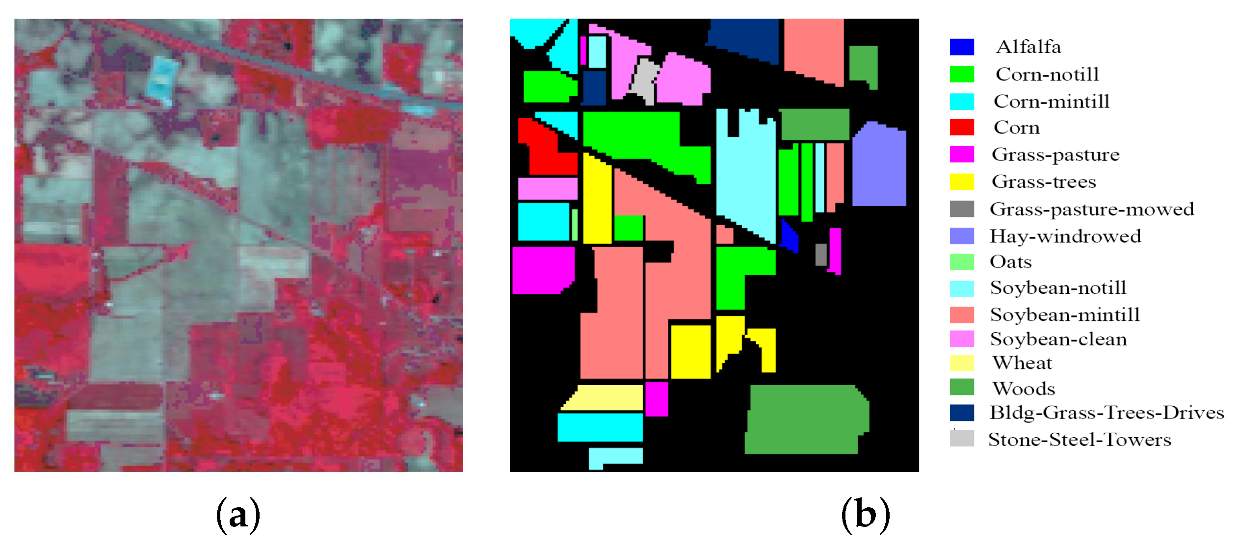
Indian Pines (IP) (ftp://ftp.ecn.purdue.edu/biehl/MultiSpec/92AV3C.tif.zip, accessed on 8 October 2015): These data have a size of 145 × 145 pixels and 220 spectral bands. After 20 bad bands are removed, the remaining 200 bands are used. The IP data contain 16 land cover classes. The false color composite image and ground-truth map are shown in Figure 2.
(2)
University of Pavia (UP) (https://www.ehu.eus/ccwintco/index.php?title=Hyperspectral_Remote_Sensing_Scenes, accessed on 8 June 2013): The UP data has the size of 610 × 340 pixels and 115 spectral bands. After 12 bad bands are discared, 103 bands are retained. The data contain nine ground-truth classes. The false color composition image and the ground-truth map are shown in Figure 3.
(3)
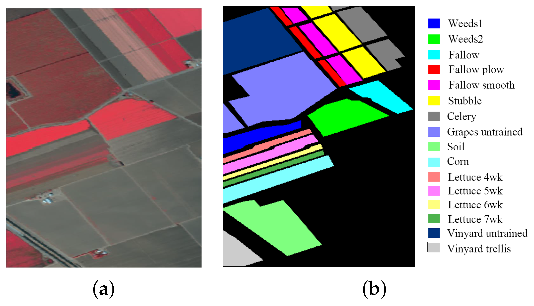
Salinas (SA) (https://www.ehu.eus/ccwintco/index.php?title=Hyperspectral_Remote_Sensing_Scenes, accessed on 8 June 2013): The SA data have a size of 512 × 217 pixels and 204 spectral bands. The data contain 16 ground-truth classes. The false color composite image and the ground-truth map are shown in Figure 4.

3.2. Experimental Setting

The proposed LMFKJSR is compared with the following classification methods: SVM with composite kernel (SVM-CK) [15], local covariance matrix representation (LCMR) [7], local correntropy matrix representation (LCEM) [30], attention-based adaptive spectral-spatial kernel improved residual network (A2S2K-ResNet, A2S2K for short) [24], NoiseCNN [26], JSR [19], kernel-based JSR (KJSR) [33], self-paced KJSR (SPKJSR) [39], covariance feature-based KJSR (LogEKJSR, here called as CovKJSR) [27], correntropy feature-based KJSR (CEKJSR). It should be noted that LCMR and LCEM are SVM classifiers performed on the local covariance matrix features and local correntropy matrix features, respectively. CovKJSR and CEKJSR are KJSR classifiers performed on local covariance and correntropy matrix features, respectively. CovKJSR and CEKJSR are special cases of the proposed LMFKJSR (CEKJSR is also our proposed method). A2S2K and NoiseCNN are recently proposed deep learning HSI classification methods. The class-specific accuracy (CA), average accuracy (AA), overall accuracy (OA), and κ coefficient on the testing set were used for comparison.
Next, in [27], in the local neighborhood construction for local feature representation and joint sparse representation, the window sizes w 1 and w 2 are set to 9, and the number of similar pixels are set as m 1 = 70 and m 2 = 30 , respectively. The sparsity level in KJSR is set as K = 40 .

3.3. Classification Results

3.3.1. Results from IP

For IP data, 1% labeled samples per class were randomly selected for training (in total, 115 training samples) and the other samples were used for testing. All methods were randomly run ten times, and the averaged classification are reported in Table 1.
From the results, we can see that:
(1)
Among the three SVM-based classifiers, the matrix-feature-based classifiers (LCMR and LCEM) show much better results than the vector-feature-based SVM-CK. This demonstrates that the local covariance or correntropy matrix feature representation is more effective than the vector feature representation. In addition, due to the strong nonlinearity similarity representation ability, LCEM shows much better results than LCMR.
(2)
The recently proposed deep HSI classification methods (A2S2K and NoiseCNN) show poor results due to the limited number of training samples. In particular, for Classes 7 and 9 with only three training samples, the OA of each method is lower than 50%. To achieve satisfactory results, deep learning methods usually need a large number of training samples.
(3)
By mining nonlinear relations between pixels, KJSR improves JSR. By further selecting similar pixels in the spatial neighborhood based on self-paced learning, SPKJSR improves KJSR. By exploiting matrix representations, CovKJSR and CEKJSR improve the traditional vector-feature-based KJSRs. CEKJSR shows better results than CovKJSR.
(4)
Comparing CovKJSR with LCMR (or CEKJSR with LCEM), it can be seen that the KJSR methods show better results than SVM-based methods on these data. For IP data, there are many large homogeneous regions and region-based characteristics that can be used to improve the classification performance. Different from LCMR and LCEM, which only use the region-based matrix features, CovKJSR and CEKJSR use region-based characteristics in both the feature and classification parts. Therefore, KJSR methods show relatively better results.
(5)
By combining the local covariance and correntropy matrix features, the proposed LMFKJSR improves both methods and provides the best results. It demonstrates that the local covariance and correntropy features are complementary.
(6)
On the subclasses of “Corn” (Classes 2, 3, 4) and “Soybean” (Classes 10, 11, 12), the proposed LMFKJSR provides overall better results than the other methods (i.e., the best results on Classes 2, 10, and 11, the second best results on Classes 3 and 4). The results demonstrate that the local matrix feature representations exploiting both spectral correlation with covariance features and band similarity with correntropy features are more effective in distinguishing the subtle differences between similar materials.
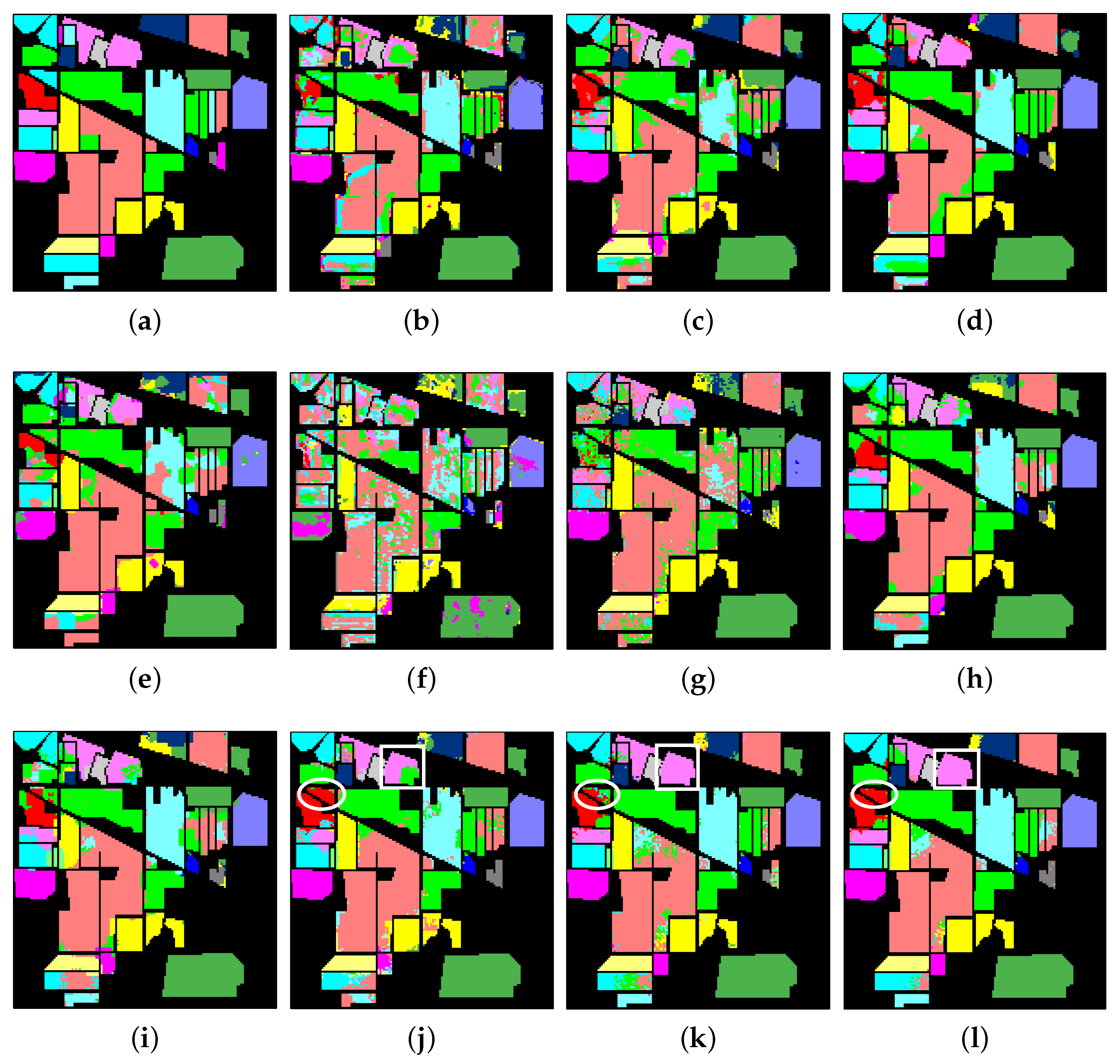
The classification maps of different methods are shown in Figure 5. By seeing the highlighted elliptic and rectangle regions in the CovKJSR, CEKJSR, and LMFKJSR maps, we can find that LMFKJSR takes advantages of CovKJSR and CEKJSR. CovKJSR shows better results on the elliptic region, while CEKJSR is much better in the rectangular region. LMFKJSR shows consistently better results in both regions. In general, the classification map of LMFKJSR is more consistent with the groundtruth map.

3.3.2. Results from UP

Because the UP data have a large number of samples, only 0.1% labeled samples per class were randomly selected for training (in total, 50 training samples), and the other samples were used for testing. The averaged classification results over ten runs are recorded in Table 2. When there were only 50 training samples, the traditional JSR-based methods showed worse results than SVM-based methods because the dictionary representation ability is insufficient in the case of limited training samples (i.e., the number of dictionary atoms is limited). The deep learning methods produce very poor results because of the lack of training samples. By combining the local covariance and correntropy matrix features, the proposed LMFKJSR method provides the best results. Compared with the KJSR-based methods, LMFKJSR improves the OA by 10% and the κ coefficient by about 13%. Although LMFKJSR provides the best results on only two classes, it has the highest AA. This shows that LMFKJSR can generate more consistent and stable results on different classes.
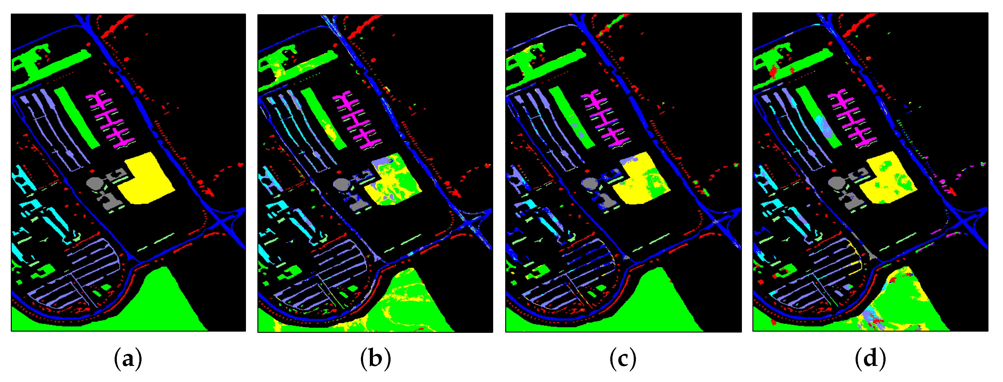
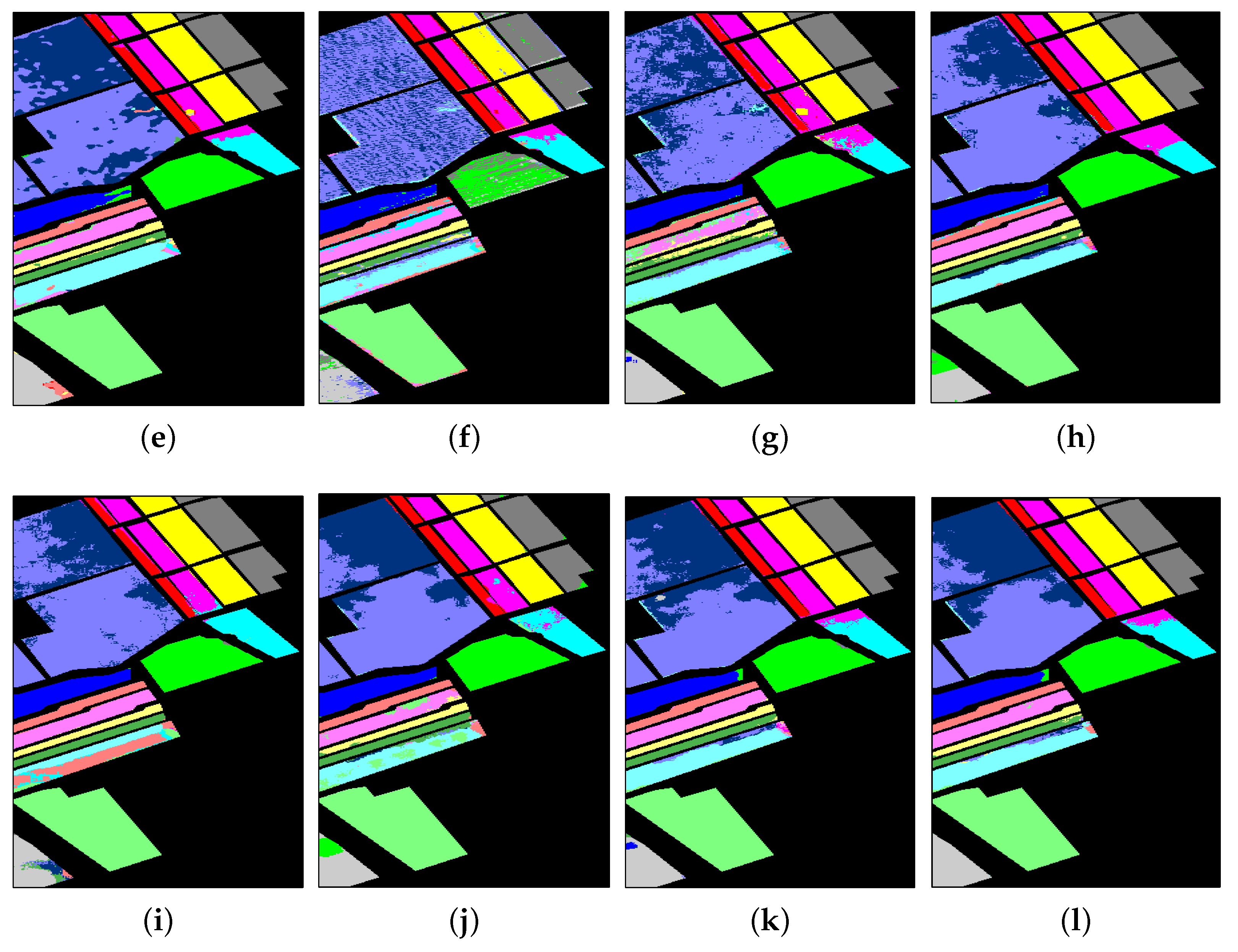
Figure 6 shows the classification maps of different methods, where the proposed LMFKJSR produces a relatively better map than other methods with little “salt and pepper” noise.

3.3.3. Results from SA

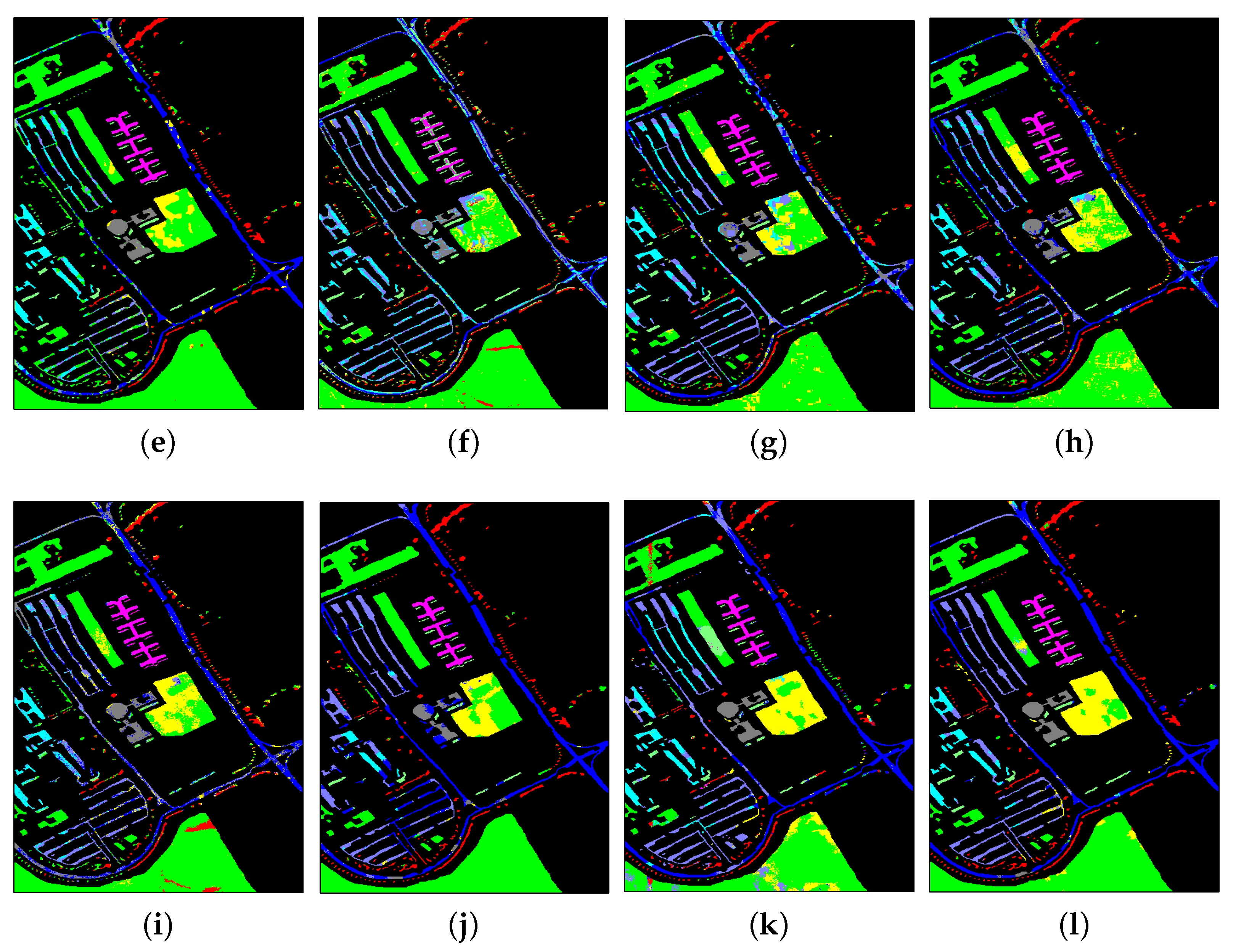
For SA data, only 0.1% labeled samples per class were randomly selected for training (totally, 66 training samples), and the other samples were used for testing. The averaged classification results over ten runs are recorded in Table 3. Except for the NoiseCNN, all methods provide OAs higher than 80%. The LMFKJSR and A2S2K provide the best and second best results. The classification of Classes 8 and 15 (i.e., “Grapes untrained” and “Vinyard untrained”) is relatively difficult for the SA data. The traditional JSR methods show poor results on Class 15, while the matrix-feature-based KJSR methods improve the traditional JSR methods by almost 20% in OA. From the classification maps in Figure 7, it can be seen that Classes 8 and 15 are located on the upper left of the image and are spatially adjacent; our proposed LMFKJSR provides better results in these two classes.

4. Discussions

4.1. The Effect of the Number of Training Samples

Here, the effect of the number of training samples on different methods is analyzed. For IP, the ratios of labeled samples per class are set as 1%, 2%, 3%, 4%, and 5%. As UP and SA have more labeled samples than IP, and the ratios of labeled samples per class are relatively smaller, i.e., 0.1%, 0.2%, 0.3%, 0.4%, and 0.5%. The OAs of different methods such as the changes in the ratio of training samples per class are shown in Figure 8. It can be seen that the proposed LMFKJSR shows consistently better results than other methods in different numbers of training samples.

4.2. The Effect of the MNF Dimension

Figure 9 shows the OA of LMFKJSR versus the MNF dimension d. It can be clearly seen that the OA dramatically increases as the of the number of dimension d increases and becomes stable when the dimension d is larger than 25. In the experiments, the dimension d is set as 25.

4.3. The Effect of the Weighting Coefficient

The proposed LMFKJSR exploits the local matrix feature, which is a combination of local covariance matrix feature and local correntropy matrix feature. The combination coefficient μ in Equation (11) measures the importance of local covariance and correntropy features. Figure 10 shows the effect of parameter μ on the LMFKJSR, where μ changes from 0 to 1 with an increment 0.1. The best μ values for three data sets are 0.9, 0.7, and 0.7, respectively. It should be noted that LMFKJSR is reduced to CEKJSR and CovKJSR in the case of μ = 0 and μ = 1 , respectively. The OA of LMFKJSR at the optimal parameter is obviously better than either CEKJSR or CovKJSR.

5. Conclusions

In this paper, a local matrix-feature-based kernel joint sparse representation (LMFKJSR) model has been proposed for hyperspectral image classification. In the proposed LMFKJSR, a novel local matrix feature (LMF) is designed to reflect both the correlation between spectral pixels and the spectral bands. In detail, the local matrix feature is a linear combination of the local covariance matrix feature and the local correntropy matrix feature, where the former can describe the correlation between spectral pixels and the latter measures the similarity between spectral bands in a local spatial neighborhood. Based on the constructed LMFs, a simple linear kernel is introduced to measure the similarity between them, and a KJSR model is performed for classification. Compared with existing vector-feature-based and matrix-feature-based SVM and JSR methods, the proposed LMFKJSR shows better results on three well-known HSI data sets.

Author Contributions

Conceptualization, X.C., N.C., J.P. and W.S.; Methodology, X.C., N.C. and J.P.; Software, X.C. and J.P.; Validation, X.C. and J.P.; Formal analysis, X.C., N.C., J.P. and W.S.; Investigation, X.C. and J.P.; Resources, J.P. and W.S.; Writing—original draft preparation, X.C., N.C. and J.P.; Writing—review and editing, X.C., N.C., J.P. and W.S.; Supervision, J.P. and W.S. All authors have read and agreed to the published version of the manuscript.

Funding

This research was funded by the National Natural Science Foundation of China under Grant Nos. 42171351, 42122009, 41971296, and by the Natural Science Foundation of Hubei Province under Grant 2021CFA087.

Data Availability Statement

Indian Pines data set is available at ftp://ftp.ecn.purdue.edu/biehl/MultiSpec/92AV3C.tif.zip, accessed on 5 October 2015. University of Pavia and Salinas data sets are available at http://www.ehu.eus/ccwintco/index.phptitle=Hyperspectral_Remote_Sensing_Scenes, accessed on 8 June 2013.

Conflicts of Interest

The authors declare no conflict of interest.

References

  1. Bioucas-Dias, J.M.; Plaza, A.; Camps-Valls, G.; Scheunders, P.; Nasrabadi, N.; Chanussot, J. Hyperspectral remote sensing data analysis and future challenges. IEEE Geosci. Remote Sens. Mag. 2013, 1, 6–36. [Google Scholar] [CrossRef]
  2. He, L.; Li, J.; Liu, C.; Li, S. Recent advances on spectral-spatial hyperspectral image classification: An overview and new guidelines. IEEE Trans. Geosci. Remote Sens. 2018, 56, 1579–1597. [Google Scholar]
  3. Peng, J.; Sun, W.; Li, H.; Li, W.; Meng, X.; Ge, C.; Du, Q. Low-rank and sparse representation for hyperspectral image processing: A review. IEEE Geosci. Remote Sens. Mag. 2022, 10, 10–43. [Google Scholar]
  4. Benediktsson, J.A.; Pesaresi, M.; Arnason, K. Classification and feature extraction for remote sensing images from urban areas based on morphological transformations. IEEE Trans. Geosci. Remote Sens. 2003, 41, 1940–1949. [Google Scholar] [CrossRef]
  5. Huang, X.; Zhang, L. An SVM ensemble approach combining spectral, structural, and semantic features for the classification of high-resolution remotely sensed imagery. IEEE Trans. Geosci. Remote Sens. 2013, 51, 257–272. [Google Scholar] [CrossRef]
  6. Zhou, Y.; Peng, J.; Chen, C.L.P. Dimension reduction using spatial and spectral regularized local discriminant embedding for hyperspectral image classification. IEEE Trans. Geosci. Remote Sens. 2015, 53, 1082–1095. [Google Scholar]
  7. Fang, L.; He, N.; Li, S.; Plaza, A.; Plaza, J. A new spatial-spectral feature extraction method for hyperspectral images using local covariance matrix representation. IEEE Trans. Geosci. Remote Sens. 2018, 56, 3534–3546. [Google Scholar] [CrossRef]
  8. Rasti, B.; Hong, D.; Hang, R.; Ghamisi, P.; Kang, X.; Chanussot, J.; Benediktsson, J.A. Feature extraction for hyperspectral imagery: The evolution from shallow to deep: Overview and toolbox. IEEE Geosci. Remote Sens. Mag. 2020, 8, 60–88. [Google Scholar] [CrossRef]
  9. Jia, S.; Zhan, Z.; Zhang, M.; Xu, M.; Huang, Q.; Zhou, J.; Jia, X. Multiple feature-based superpixel-level decision fusion for hyperspectral and LiDAR data classification. IEEE Trans. Geosci. Remote Sens. 2021, 59, 1437–1452. [Google Scholar]
  10. Melgani, F.; Bruzzone, L. Classification of hyperspectral remote sensing images with support vector machines. IEEE Trans. Geosci. Remote Sens. 2004, 42, 1778–1790. [Google Scholar] [CrossRef]
  11. Camps-Valls, G.; Bruzzone, L. Kernel-based methods for hyperspectral image classification. IEEE Trans. Geosci. Remote Sens. 2005, 43, 1351–1362. [Google Scholar] [CrossRef]
  12. Shen, L.; Jia, S. Three-dimensional Gabor wavelets for pixel-based hyperspectral imagery classification. IEEE Trans. Geosci. Remote Sens. 2011, 49, 5039–5046. [Google Scholar] [CrossRef]
  13. Li, W.; Chen, C.; Su, H.; Du, Q. Local binary patterns and extreme learning machine for hyperspectral imagery classification. IEEE Trans. Geosci. Remote Sens. 2015, 53, 3681–3693. [Google Scholar] [CrossRef]
  14. Borzov, S.; Potaturkin, O. Increasing the classification efficiency of hyperspectral images due to multi-scale spatial processing. Comput. Opt. 2020, 44, 937–943. [Google Scholar]
  15. Camps-Valls, G.; Gomez-Chova, L.; Munoz-Mare, J.; Vila-Frances, J.; Calpe-Maravilla, J. Composite kernels for hyperspectral image classification. IEEE Geosci. Remote Sens. Lett. 2006, 3, 93–97. [Google Scholar] [CrossRef]
  16. Peng, J.; Zhou, Y.; Chen, C.L.P. Region-kernel-based support vector machines for hyperspectral image classification. IEEE Trans. Geosci. Remote Sens. 2015, 53, 4810–4824. [Google Scholar]
  17. Zhou, Y.; Peng, J.; Chen, C.L.P. Extreme learning machine with composite kernels for hyperspectral image classification. IEEE J. Sel. Top. Appl. Earth Obs. Remote Sens. 2015, 8, 2351–2360. [Google Scholar]
  18. Gu, Y.; Chanussot, J.; Jia, X.; Benediktsson, J.A. Multiple kernel learning for hyperspectral image classification: A review. IEEE Trans. Geosci. Remote Sens. 2017, 55, 6547–6565. [Google Scholar] [CrossRef]
  19. Chen, Y.; Nasrabadi, N.; Tran, T. Hyperspectral image classification using dictionary-based sparse representation. IEEE Trans. Geosci. Remote Sens. 2011, 49, 3973–3985. [Google Scholar]
  20. Peng, J.; Du, Q. Robust joint sparse representation based on maximum correntropy criterion for hyperspectral image classification. IEEE Trans. Geosci. Remote Sens. 2017, 55, 7152–7164. [Google Scholar]
  21. Peng, J.; Sun, W.; Du, Q. Self-paced joint sparse representation for the classification of hyperspectral images. IEEE Trans. Geosci. Remote Sens. 2019, 57, 1183–1194. [Google Scholar] [CrossRef]
  22. Li, W.; Du, Q. Joint within-class collaborative representation for hyperspectral image classification. IEEE J. Sel. Top. Appl. Earth Obs. Remote Sens. 2014, 7, 2200–2208. [Google Scholar] [CrossRef]
  23. Zhang, L.; Zhang, L.; Du, B. Deep learning for remote sensing data: A technical tutorial on the state of the art. IEEE Geosci. Remote Sens. Mag. 2016, 4, 22–40. [Google Scholar] [CrossRef]
  24. Roy, S.; Manna, S.; Song, T.; Bruzzone, L. Attention-based adaptive spectral–spatial kernel ResNet for hyperspectral image classification. IEEE Trans. Geosci. Remote Sens. 2021, 59, 7831–7843. [Google Scholar] [CrossRef]
  25. Chen, Y.; Jiang, H.; Li, C.; Jia, X.; Ghamisi, P. Deep feature extraction and classification of hyperspectral images based on convolutional neural networks. IEEE Trans. Geosci. Remote Sens. 2016, 54, 6232–6251. [Google Scholar] [CrossRef]
  26. Gong, Z.; Zhong, P.; Qi, J.; Hu, P. A CNN with noise inclined module and denoise framework for hyperspectral image classification. arXiv 2022, arXiv:2205.12459. [Google Scholar]
  27. Yang, W.; Peng, J.; Sun, W.; Du, Q. Log-Euclidean kernel-based joint sparse representation for hyperspectral image classification. IEEE J. Sel. Top. Appl. Earth Obs. Remote Sens. 2019, 12, 5023–5034. [Google Scholar] [CrossRef]
  28. Tabia, H.; Laga, H. Covariance-based descriptors for efficient 3D shape matching, retrieval, and classification. IEEE Trans. Multimed. 2015, 17, 1591–1603. [Google Scholar] [CrossRef]
  29. Tuzel, O.; Porikli, F.; Meer, P. Region covariance: A fast descriptor for detection and classification. In Proceedings of the European Conference on Computer Vision (ECCV), Graz, Austria, 7–13 May 2006; pp. 589–600. [Google Scholar]
  30. Zhang, X.; Wei, Y.; Cao, W.; Yao, H.; Peng, J.; Zhou, Y. Local correntropy matrix representation for hyperspectral image classification. IEEE Trans. Geosci. Remote Sens. 2022, 60, 5525813. [Google Scholar] [CrossRef]
  31. Liu, W.; Pokharel, P.P.; Príncipe, J.C. Correntropy: Properties and applications in non-Gaussian signal processing. IEEE Trans. Signal Process. 2007, 55, 5286–5298. [Google Scholar] [CrossRef]
  32. Peng, J.; Li, L.; Tang, Y. Maximum likelihood estimation based joint sparse representation for the classification of hyperspectral remote sensing images. IEEE Trans. Neural Netw. Learn. Syst. 2019, 30, 1790–1802. [Google Scholar] [CrossRef] [PubMed]
  33. Chen, Y.; Nasrabadi, N.; Tran, T. Hyperspectral image classification via kernel sparse representation. IEEE Trans. Geosci. Remote Sens. 2013, 51, 217–231. [Google Scholar] [CrossRef]
  34. Green, A.; Berman, M.; Switzer, P.; Craig, M.D. A transformation for ordering multispectral data in terms of image quality with implications for noise removal. IEEE Trans. Geosci. Remote Sens. 1998, 26, 65–74. [Google Scholar] [CrossRef]
  35. Zhang, H.; Li, J.; Huang, Y.; Zhang, L. A nonlocal weighted joint sparse representation classification method for hyperspectral imagery. IEEE J. Sel. Top. Appl. Earth Obs. Remote Sens. 2014, 7, 2057–2066. [Google Scholar] [CrossRef]
  36. Fang, L.; Li, S.; Duan, W.; Ren, J.; Benediktsson, J.A. Classification of hyperspectral images by exploiting spectral–spatial information of superpixel via multiple kernels. IEEE Trans. Geosci. Remote Sens. 2015, 53, 6663–6674. [Google Scholar] [CrossRef]
  37. Li, P.; Wang, Q.; Zeng, H.; Zhang, L. Local Log-Euclidean multivariate Gaussian descriptor and its application to image classification. IEEE Trans. Pattern Anal. Machiche Intell. 2017, 39, 803–817. [Google Scholar] [CrossRef] [PubMed]
  38. Li, P.; Wang, Q.; Zuo, W.; Zhang, L. Log-Euclidean kernels for sparse representation and dictionary learningn. In Proceedings of the International Conference on Computer Vision (ICCV), Sydney, Australia, 1–8 December 2013; pp. 1601–1608. [Google Scholar]
  39. Hu, S.; Peng, J.; Fu, Y.; Li, L. Kernel joint sparse representation based on self-paced learning for hyperspectral image classification. Remote Sens. 2019, 11, 1114. [Google Scholar] [CrossRef] [Green Version]
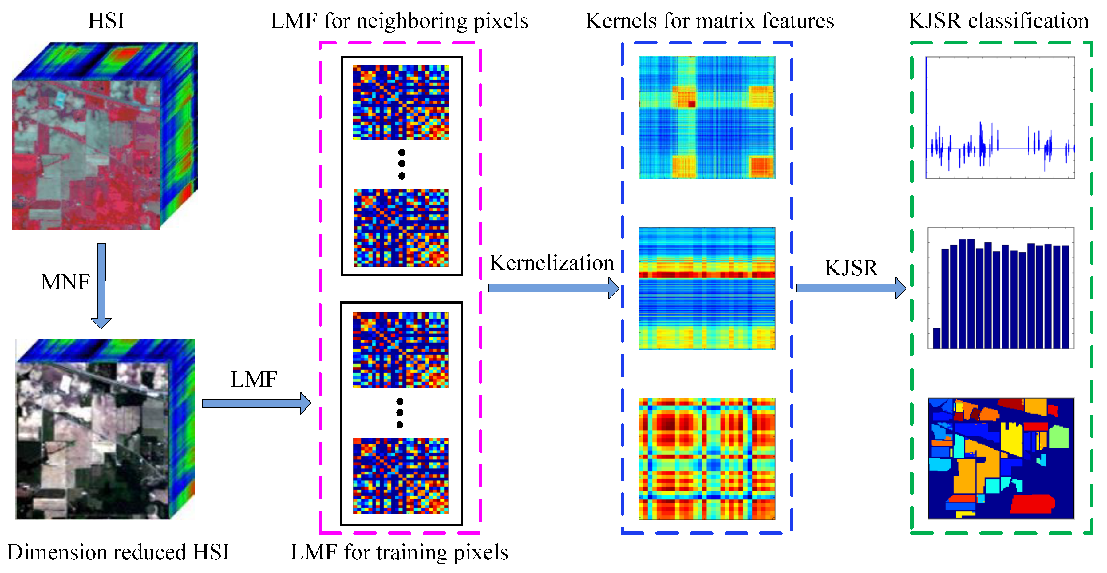
Figure 1. The framework of the proposed LMFKJSR algorithm, which mainly consists of three steps, i.e., maximum noise fraction-based dimensionality reduction, local matrix feature extraction, and matrix kernel-based JSR classification.
Remotesensing 14 04363 g001
Figure 2. IP data set: (a) RGB composite image; (b) Ground-truth map.
Remotesensing 14 04363 g002
Figure 3. UP data set: (a) RGB composite image; (b) Ground-truth map.
Remotesensing 14 04363 g003
Figure 4. SA data set: (a) RGB composite image; (b) Ground-truth map.
Remotesensing 14 04363 g004
Figure 5. Classification maps on IP: (a) Groundtruth, (b) SVMCK, (c) LCMR, (d) LCEM, (e) A2S2K, (f) NoiseCNN, (g) JSR, (h) KJSR, (i) SPKJSR, (j) CovKJSR, (k) CEKJSR, (l) LMFKJSR.
Remotesensing 14 04363 g005
Figure 6. Classification maps on UP: Classification maps on IP: (a) Groundtruth, (b) SVMCK, (c) LCMR, (d) LCEM, (e) A2S2K, (f) NoiseCNN, (g) JSR, (h) KJSR, (i) SPKJSR, (j) CovKJSR, (k) CEKJSR, (l) LMFKJSR.
Remotesensing 14 04363 g006aRemotesensing 14 04363 g006b
Figure 7. Classification maps on SA. Classification maps on IP: (a) Groundtruth, (b) SVMCK, (c) LCMR, (d) LCEM, (e) A2S2K, (f) NoiseCNN, (g) JSR, (h) KJSR, (i) SPKJSR, (j) CovKJSR, (k) CEKJSR, (l) LMFKJSR.
Remotesensing 14 04363 g007aRemotesensing 14 04363 g007b
Figure 8. The OA versus the ratio of training samples per class: (a) IP; (b) UP; (c) SA.
Remotesensing 14 04363 g008
Figure 9. The OA versus the MNF dimension d: (a) IP; (b) UP; (c) SA.
Remotesensing 14 04363 g009
Figure 10. The OA versus the weighting coefficient μ : (a) IP; (b) UP; (c) SA.
Remotesensing 14 04363 g010
Table 1. Classification results on the IP data set with 1% labeled training samples (115 training samples). The bold values indicate the highest accuracy among all methods.
ClassTrainTestSVMCKLCMRLCEMA2S2KNoiseCNNJSRKJSRSPKJSRCovKJSRCEKJSRLMFKJSR
135164.1299.2293.9486.6746.1577.8488.0496.6797.0692.1695.69
214142075.4575.6889.6668.1248.8658.4070.5778.1183.6890.8094.05
3882661.1157.0371.4488.3237.0740.1158.6866.2369.6276.2783.00
4323156.0273.8578.9289.2672.0936.3658.7077.1982.9080.6584.11
5549270.8771.6983.4686.9658.3368.7275.2277.7680.7783.4484.59
6774085.5478.1295.2892.0857.5896.9595.1887.5885.2095.4297.43
732393.04100.0100.049.028.5458.7085.65100.0100.0100.0100.0
8548488.5994.3697.1297.4282.9989.6797.9198.3198.5198.1299.79
931789.41100.0100.034.6922.2231.1851.1890.00100.0100.0100.0
101095862.4657.3976.8180.5231.4640.4576.8280.0471.3686.1088.80
1125244379.7883.9888.6971.0549.2678.7086.3988.2689.8289.8391.47
12660845.7651.8971.9390.8326.6942.4856.8166.6070.5483.1182.68
13320983.2184.8898.4287.0742.3698.9599.9584.4084.5599.3899.86
1413128192.4594.0494.3686.8979.2798.5199.0298.0998.7595.1596.66
15437654.3970.4579.3470.7046.5146.5237.2654.7676.9983.2283.80
1639296.5293.8095.7675.8647.6294.1387.0784.4694.5799.3599.24
Overall accuracy74.7576.5386.4378.9051.5869.1879.3482.6684.8289.1691.36
Average accuracy74.9280.4088.4478.4747.3366.1076.5383.0387.1590.8192.57
Coefficient κ 0.7120.7300.8450.7570.4390.6440.7620.8010.8260.8760.902
Table 2. Classification results on the UP data set with 0.1% labeled training samples (50 training samples). The bold values indicate the highest accuracy among all methods.
ClassTrainTestSVMCKLCMRLCEMA2S2KNoiseCNNJSRKJSRSPKJSRCovKJSRCEKJSRLMFKJSR
17662474.5483.4784.6776.7864.2431.0168.1373.9180.9177.7283.38
2191863088.8199.1489.7173.8683.8290.0390.4889.8999.6484.2697.92
33209663.1966.8268.7656.7429.1067.5665.8467.2951.5773.7879.90
43306174.9386.2363.7697.6182.9875.2674.0164.4085.4761.0080.00
53134299.6189.5297.7698.8297.2799.6999.8499.3399.3099.5299.57
65502450.6369.7783.3574.8561.6131.6944.9650.5955.5577.5982.95
73132779.1677.1296.6773.2413.2080.7866.4474.1574.62100.099.01
84367862.7862.4964.8557.2448.6864.8347.6149.9346.8166.5373.13
9394486.2998.5593.8155.5531.1978.8877.7812.0369.4171.0490.91
Overall accuracy77.6086.5983.7174.0565.8169.4674.8575.2982.1779.4389.53
Average accuracy75.5581.4682.5973.8556.8968.8673.7164.6173.7079.0587.42
Coefficient κ 0.7020.8190.7860.6330.5410.5900.6610.6670.7550.7330.860
Table 3. Classification results for the Salinas data set with 0.1% labeled training samples (66 training samples). The bold values indicate the highest accuracy among all methods.
ClassTrainTestSVMCKLCMRLCEMA2S2KNoiseCNNJSRKJSRSPKJSRCovKJSRCEKJSRLCCKJSR
13200689.8298.8499.4099.9788.6399.7999.8699.9199.9199.2799.21
24372294.3490.7498.7698.3292.1699.0199.8199.2793.5999.2499.86
33197374.3596.1593.5897.1774.2778.8676.9083.0295.3995.9795.48
43139192.5893.9097.2891.4083.0598.0794.2886.2497.0498.2798.68
53267579.9764.8599.1986.7184.2285.7694.0595.9073.7999.2798.37
64395596.9395.6399.9099.8099.1899.87100.099.8699.8199.9099.89
74357594.9592.58100.099.5073.8999.9399.68100.098.8899.9999.94
8111126081.9587.4877.8981.6154.7990.7687.0789.9688.0982.2489.09
96619794.0798.4899.9198.9299.1199.9599.7899.9799.8599.97100.0
103327552.6753.9572.2397.7085.3092.4859.9563.7664.6570.5670.36
113106590.0180.4596.8590.7865.5794.4287.1999.5998.5799.2599.66
123192485.4771.8391.4995.8981.4379.0797.4294.4583.8594.1093.79
13391397.0294.6699.1293.4088.2579.8999.6796.9095.4997.8399.19
143106793.8785.8197.2392.3398.0295.4998.8699.7687.6797.9695.91
157726178.0265.7578.8978.5737.7854.3153.6652.0473.5674.7373.13
163180466.4679.0092.2197.9669.1499.0581.0185.1088.8787.8888.65
Overall accuracy84.2983.8489.7190.9573.2783.6486.3087.2788.4490.1091.29
Average accuracy85.1684.3893.3793.7579.6784.7489.3290.3689.9493.5393.83
Coefficient κ 0.8250.8190.8850.8990.7010.8170.8470.8580.8710.8900.903
Publisher’s Note: MDPI stays neutral with regard to jurisdictional claims in published maps and institutional affiliations.