Article

Estimating Rangeland Fine Fuel Biomass in Western Texas Using High-Resolution Aerial Imagery and Machine Learning

1
Department of Ecology and Conservation Biology, Texas A&M University, College Station, TX 77843, USA
2
USDA Agricultural Research Service, Fort Keogh Livestock and Range Research Laboratory, Miles City, MT 59301, USA
3
USDA Agricultural Research Service, Southern Plains Agricultural Research Center, College Station, TX 77845, USA
*
Author to whom correspondence should be addressed.
Remote Sens. 2022, 14(17), 4360; https://doi.org/10.3390/rs14174360
Submission received: 26 July 2022 / Revised: 29 August 2022 / Accepted: 29 August 2022 / Published: 2 September 2022
(This article belongs to the Section Remote Sensing in Agriculture and Vegetation)

Abstract

:
Rangeland fine fuel biomass is a key factor in determining fire spread and intensity, while the accuracy of biomass estimation is limited due to inherent heterogeneity in rangeland ecosystems. In this study, high spatial resolution (0.23 m) images were used to classify fuel types and predict rangeland fine fuel biomass in west Texas based on the random forest algorithm. Two biomass models, including one with the fuel type, original spectral bands, and vegetation indices as explanatory variables, and the other that contained a combination of the fuel type, original spectral bands, vegetation, and texture indices as explanatory variables, were assessed. Furthermore, the biomass models were also examined by upscaling the remote sensing images from high to medium (30 m) spatial resolution with the spectral curves derived from Landsat images. The fuel type map had an accuracy of more than 95%, and herbaceous fuel types were kept for estimating fine fuel biomass. The results showed that around 76% and 80% of biomass variances were explained by models without texture indices and with texture indices, respectively. The fuel type and the normalized difference vegetation index (NDVI) were two significant input variables influencing fine fuel biomass for both models and adding texture indices contributed to the improvement of model accuracy. An upscaling analysis for biomass estimation using medium spatial resolution imagery showed that approximately 60% of the variance in biomass was explained by the model. The addition of fractional vegetation cover improved the model performance by explaining an additional 5% of the variance in biomass estimation. These findings indicate that high spatial resolution images have the potential to effectively estimate rangeland fuel types and fine fuel biomass, which can be helpful for mapping the spatial distribution of fine fuels to aid in monitoring and fire management on rangelands.

Graphical Abstract

1. Introduction

Rangelands, which are comprised of grasses, grasslike plants, forbs, or shrubs in arid and semiarid regions, occupy almost half of the global terrestrial lands [1,2,3], and provide a broad diversity of provisioning, supporting, regulating, and cultural services on these lands [4,5]. Fire is a significant component of many rangeland ecosystems [6], which can lead to spatial and temporal variability in rangeland structure [7,8]. Rangeland biomass, which is a critical factor influencing the spread and intensity of fires, is widely used as an input variable for fire behavior models [9,10,11]. Fine fuels and fuel types are the main vegetation parameters in fire behavior models and better understanding rangeland conditions can help better predict fire behaviors and estimate fire impacts on rangelands [12]. The ability to map fuel types and amounts can reveal patterns in fuel that can allow better decision-making for fire management and the development of plans for prescribed burning under more favorable conditions in areas having high fuel loads [13]. Rangelands are heterogeneous and improved estimation of rangeland fine fuel biomass can help range managers adopt appropriate strategies to reduce wildfire risk and harmful impacts of wildfires on rangeland functions and services. Nevertheless, the accuracy of biomass estimation is limited due to high heterogeneity in rangeland ecosystems [12] and improving rangeland biomass estimation is greatly needed to better monitor rangeland conditions.
Traditional field biomass sampling methods are essential as they can provide true ground measurements, but they are laborious and costly, thus creating challenges for implementation over large land areas [14,15]. Remote sensing technologies offer a non-destructive way to estimate biomass over large areas and have been widely used to estimate herbaceous biomass [14,16,17,18]. Different temporal and spatial remote sensing images, such as those derived from Terra and Aqua MODIS, Landsat OLI, and Sentinel-2 MSI, have been broadly applied for predicting rangeland biomass [19,20,21]. The spatial resolution of these images is relatively coarse, and higher resolution images are needed to capture more detailed information on the variability and patterns of biomass on the landscape. High-resolution images have been widely used in agriculture [22,23,24,25], and their applications in rangeland biomass estimation are promising as they can identify fine-scale rangeland heterogeneity and could improve the accuracy of biomass estimation [22,23]. A combination of field samplings and high-resolution remote sensing images could provide a better estimation of rangeland fine fuel biomass over large areas. Satellite-based vegetation indices, which are related to vegetation biophysical characteristics, can be used as proxies of vegetation biomass [17]. The Normalized Difference Vegetation Index (NDVI) [26], which indicates vegetation greenness, has been widely used in estimating grassland biomass since the 1970s [24,25,27]. Other vegetation indices, such as the Optimized Soil Adjusted Vegetation Index (OSAVI) [16,28], Enhanced Vegetation Index (EVI) [29], Soil-Adjusted Vegetation Index (SAVI) [30], and Modified Soil-Adjusted Vegetation Index (MSAVI) [31], have also been applied to estimate grassland biomass [32]. Furthermore, texture information, which indicates the spatial arrangement of features having tonal differences in an image, can reveal various structural characteristics of images [33,34]. The inclusion of texture information from high spatial resolution images can help capture the heterogeneity of different fuel types, which could further improve the accuracy of biomass estimation [33,34,35,36].
Biomass modeling methods, such as traditional partial least squares regression and multiple linear regression algorithms, assume that field biomass measurements and spectral indices have explicit relationships that can be specified by the parameters, and these methods have been used to estimate grassland biomass [37]; however, the relationship may not be stable if the field measurements are nonlinearly related to the remote sensing variables [37] or if the assumptions of these statistical methods (e.g., normality) cannot be met. Machine learning algorithms have been used to estimate biomass as they do not need to follow assumptions about data normality and they also have the advantage of handling large numbers of variables, thus making them more appropriate to perform estimation [38,39]. Furthermore, many studies have shown the better performance of non-parametric machine learning algorithms over traditional parametric algorithms due to their ability to handle complicated relationships between biomass and various biophysical variables [40,41].
Biomass models, based on high spatial resolution images, were sometimes limited in application due to their relatively small areas of coverage. Unclear is whether these models can remain stable when estimating biomass using medium spatial resolution images. Thus, evaluating model performance at different scales can assess model stability and, if stable, enable their applications over larger areas. This study aims to estimate fine fuel biomass using high spatial resolution images and to identify the factors that have a significant influence on biomass estimation, which would include assessing the utility of texture information for improving model accuracy. Furthermore, the random forest model was assessed to examine the performance of the model when upscaling to medium-resolution remote sensing images using the spectral information derived from Landsat images. The objectives of this study were to (1) classify fuel types in rangeland ecosystems using high-resolution imagery; (2) generate fine fuel biomass maps based on different biomass models and identify variable importance in biomass estimation; (3) examine the model suitability when upscaling from high to medium spatial resolution and assess related variable importance.

2. Materials and Methods

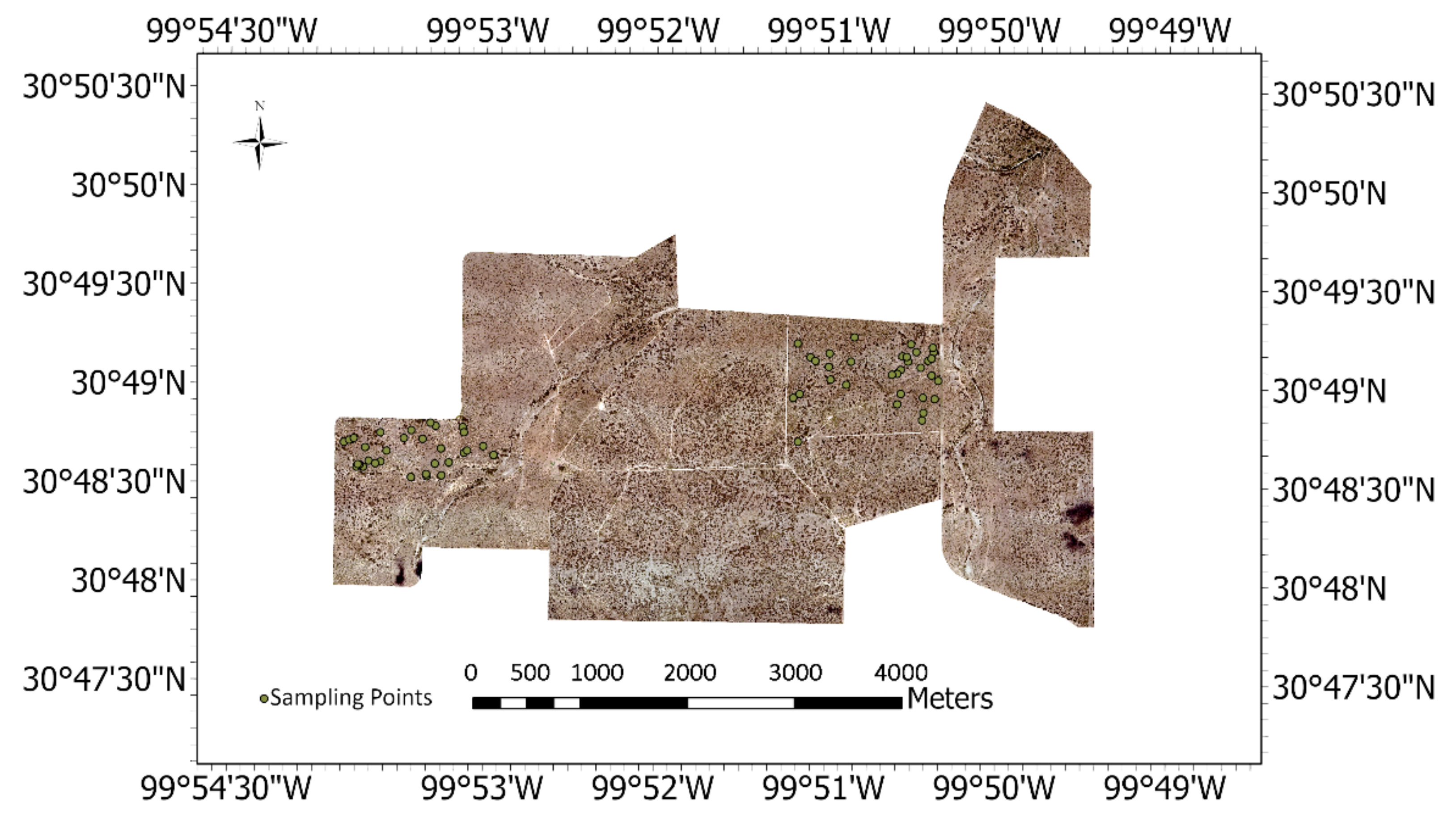
2.1. Study Area and Field Sampling

This study was conducted on the Martin Ranch (Lat 30.81N; Long −99.87W), which is approximately 1902 ha (4700 ac) in size and located in Menard County, Texas (Figure 1). The mean annual precipitation at the Martin Ranch is 640 mm, and the annual mean temperature has been 17.95 °C for the most recent three decades (1991–2020) [42]. The dominant soil is the Tarrant series [43], and the elevation ranges from 614.61 m to 677.74 m. Vegetation at the study site is described as Mesquite-Oak savanna that can be characterized as a matrix of evergreen live oak (Quercus fusiformis) tree clusters, individual honey mesquite (Prosopis glandulosa) shrubs or clusters of mesquite, and subdominant shrubs, herbaceous vegetation made up of grasses and forbs, and Opuntia spp. cacti [44]. Subdominant trees and shrubs include ashe juniper (Juniperus ashei), redberry juniper (Juniperus pinchoti), shin oak (Quercus havardii), Texas persimmon (Diospyros texana), and lotebush (Ziziphus obtusifolia). Dominant herbaceous plants at the study site include Texas wintergrass (Nassella leucotricha), sideoats grama (Bouteloua curtipendula), common curly mesquite (Hilaria belangeri), red grama (Bouteloua trifida), threeawn (Aristida spp.), hairy tridens (Erioneuron pilosum), and sedges (Carex spp.) [45].
Field biomass samplings at the study site were collected by assigning random locations within the perimeter of the ranch (67 sampling points total). At each point, herbaceous biomass within a 1-m2 quadrat was clipped to ground level and biomass was placed in paper bags. The biomass samples were then dried in a forced air oven at 65 °C for 48 h and weighted to the nearest 10th of a gram. At all sampling locations, the center of the 1-m2 quadrat was georeferenced in the field with a Trimble Geo7X having an accuracy of approximately 0.5 m. The field samples were collected over a period from 23rd October 2018 to 10th January 2019.
Figure 1. Study area and field sampling points.
Remotesensing 14 04360 g001

2.2. Remote Sensing Data Acquisition and Preprocessing

The high spatial resolution aerial images covering the study area were collected on 1st September 2018, with a Cessna 206 aircraft equipped with a Nikon D810 RGB camera and a modified Nikon D810 NIR camera. Aerial images were captured at a flight height of approximately 1981 m above mean sea level. The images were geometrically corrected and georeferenced using Pix4D software and were radiometrically calibrated with spectral curves collected from calibration tarps placed in the study area at the time of the flights. The spatial resolution of the images was 0.23 m, and four spectral bands, including Blue (B), Green (G), Red (R), and Near-infrared (NIR), were obtained. To match imagery with the 1-m2 field samplings, the pixels within the perimeter of the 1-m2 quadrat were averaged to obtain the spectral curves for B, G, R, and NIR bands for each sampled quadrat. Pixels for areas defined as roads were removed as these were not a source of biomass at this location. The random forest image classification for fuel types was based on the Scott and Burgan Fire Behavior Model [46] fuel types. Of these fuel types, the Grass Fuel Type Models (GR1, GR2), Grass-Shrub Fuel Type Model (GS2), and Timber-Understory Fuel Type Model (TU1) were selected for fuel type classification based on the vegetation conditions in the study area (Table 1) [46].
The geometrically corrected and geographically projected Landsat 8 Operational Land Imager (OLI) data were obtained from the U.S. Geological Survey (USGS) Earth Explorer website [47] for use in the biomass model upscaling analysis. The cloud-free Landsat images (Path: 28; Row: 39, Collection Date: 4th August 2018), which were nearest to the date of the high spatial resolution images, were downloaded and clipped to the boundary of the study area.

2.3. Spectral Indices

Different spectral indices, which indicate vegetation photosynthetic activity and greenness, were calculated [23,48] for both the high resolution and Landsat imagery. The selected vegetation indices were based on their performance in previous herbaceous biomass estimation studies [49,50,51]. These included NDVI, EVI, SAVI, MSAVI, and OSAVI. The spectral curves of the four original bands in the high spatial resolution images (B, G, R, and NIR) and the five spectral indices listed above that were derived from the four original bands, were evaluated in this study. The gray-level co-occurrence matrix (GLCM) method, which is used for rotation invariance and multi-scale properties, was applied to extract texture information [52]. The texture variables, including texture, mean, and variance, were derived from the high spatial resolution images of the study area using a processing window size of 5 × 5 pixels, which was near the size of the field sampled quadrats (1-m2). The equations and references for the vegetation and texture indices are shown in Table 2. The same input variables, including the fuel type, original spectral bands, vegetation, and texture indices, were used in the machine learning models for both high and medium spatial resolution images to compare the differences in spatial resolution in influencing biomass estimation.

2.4. Random Forest Classification and Regression

The Random Forest (RF) machine learning algorithm [56] was used to classify the fuel types and estimate rangeland herbaceous biomass. RF combines a large set of decision trees and creates multiple regression trees with bootstrap samples [56]. For each regression tree, “in-bag” and “out of bag” datasets are created for model training and testing (validation) [57]. The RF model reduces bias and overfitting and is more accurate than simple regression techniques [56]. RF excels at uncovering inherent relationships and structures in data with hierarchical or non-additive variables [58]. To evaluate RF model performance, the Root Mean Square Error (RMSE), the Mean Absolute Error (MAE), and variance explained were used to quantify the goodness of fit and model accuracy. The performance of the input variables was assessed by the percent increase in Mean Square Error (%IncMSE), which was calculated as the increase in Out of Bag (OOB) error when the variable was permuted [23]. The ntree, which is a parameter from the random forest algorithm, represents the number of trees grown in the model and was set to 500. The parameter mtry, which represents the number of randomly selected predictors at each node, was automatically optimized.
The fuel types were classified using random forest algorithms based on original spectral bands and vegetation indices derived from the high spatial resolution (0.23 m) remote sensing images. Four fuel types (GR1, GR2, GS2, and TU1) and shadows were included in the classification. More than 10,000-pixel samples, which were manually selected from high-resolution images, were used to classify fuel types, and each type had more than 2000 samples. Seventy percent of the sampling points were used for training the RF model, and the remaining thirty percent were used for independent testing of model performance (validation). The confusion matrix was used for accuracy assessment. The GR1 and GR2 fuel types were kept as variables for the rangeland fine fuel biomass estimation.
Two RF biomass models were assessed. One model used the fuel type (GR1 and GR2), the original spectral bands, and the derived vegetation indices as input variables for rangeland fine fuel biomass estimation, and the other model used the combination of the fuel type, original spectral bands, and vegetation and texture indices as input variables for biomass estimation. To reduce the redundancy of adding texture indices in the biomass model, the input variables, which accounted for more than 10% of the percent increase in mean square error, were used for calculating the texture indices. For the biomass modeling, 70% of the field samples were used for training the RF models, and the remaining 30% were used for independent testing of the RF model’s performance (validation). The RMSE, MAE, and R2 were used to assess model performance, and the %IncMSE was applied to represent variable importance.
To upscale from high to medium spatial resolution imagery, the fractional cover of each fuel type within each Landsat pixel was calculated from the high-resolution RF model output. The boundary for each Landsat pixel was digitized using the Fishnet tool in ArcGIS, and the Tabulate Area from Spatial Analyst Tools in ArcGIS was used to calculate the fractional cover of fuel types within each Landsat pixel. Based on the fuel type fractional cover, the pixels having more than 90% of GR1 and GR2 (i.e., fine fuel types; herbaceous vegetation) were selected, and the derived spectral curves were averaged for each fuel type. For each Landsat pixel, the spectral information for the herbaceous vegetation was calculated as the linear combination of fractional cover and spectral curves derived from the Landsat image [59]. Based on the adjusted spectral curves for herbaceous vegetation, the vegetation and texture indices were calculated using the same equations given in Table 2. Furthermore, the fractional cover of GR1 and GR2 was also included in the RF model used for upscaling herbaceous biomass. All data processing was accomplished in the R software, and the randomForest package in R was used for RF classification and regression [60].

3. Results

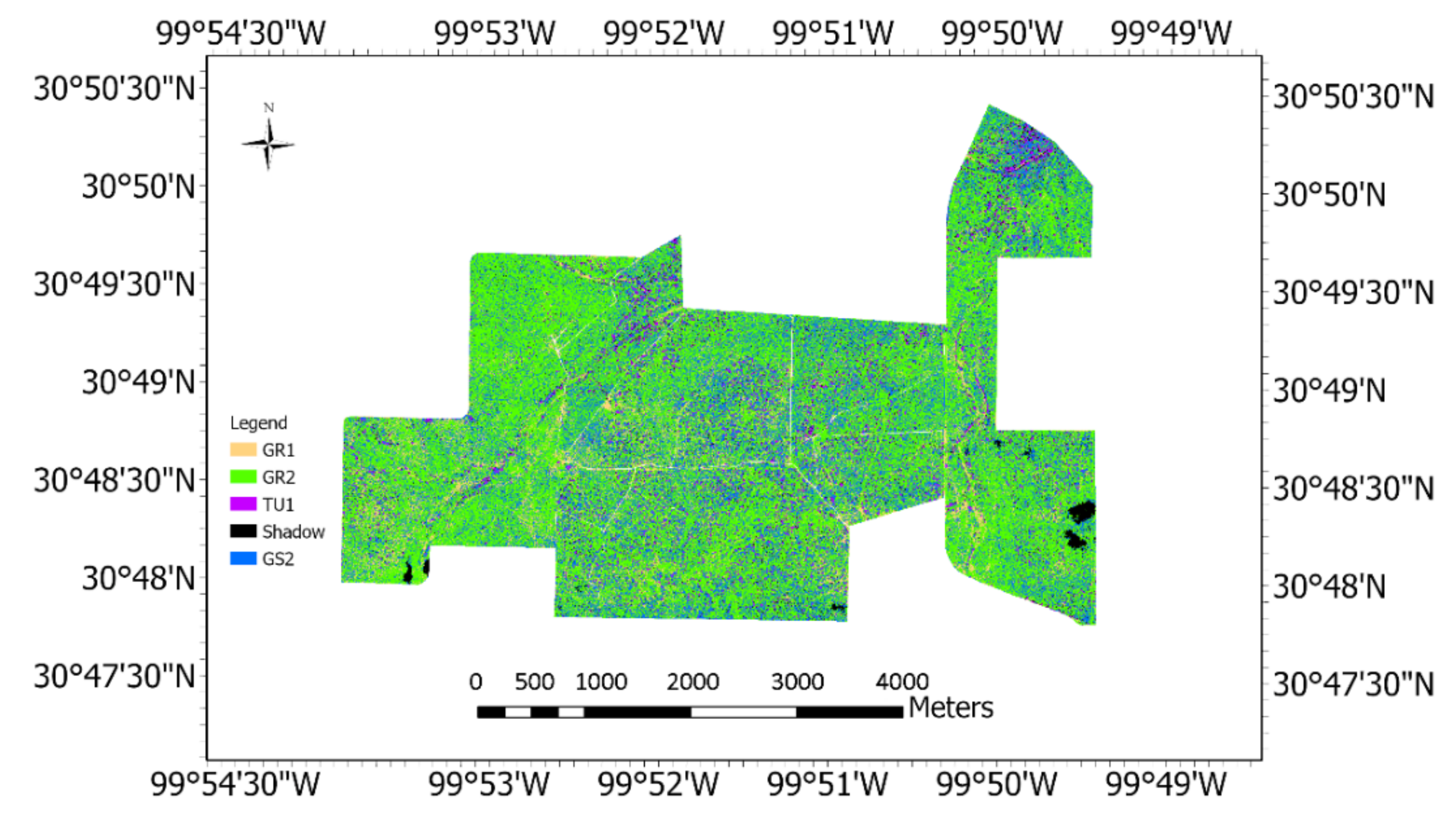
3.1. Random Forest Classification of Fuel Types

The fuel type RF classification (Figure 2) had an overall accuracy of 95.40%. The user’s accuracy ranged from 89.72% to 99.31%, and the producer’s accuracy ranged from 89.25% to 99.52%. Besides shadow, GR1 had higher user’s and producer’s accuracy (>99%) (Table 3). GR2 also had a relatively high user’s and producer’s accuracy 97%) (Table 3). GS2 and TU1 had relatively lower user’s and producer’s accuracy compared with other types, as some pixels were misclassified (Table 3). For the TU1 fuel class, the model misclassified this class with the GS2 fuel type. For the GS2 fuel type, the user’s and producer’s accuracy (~89%) was the lowest of all fuel types and had misclassifications with the TU1 and GR2 fuel types.

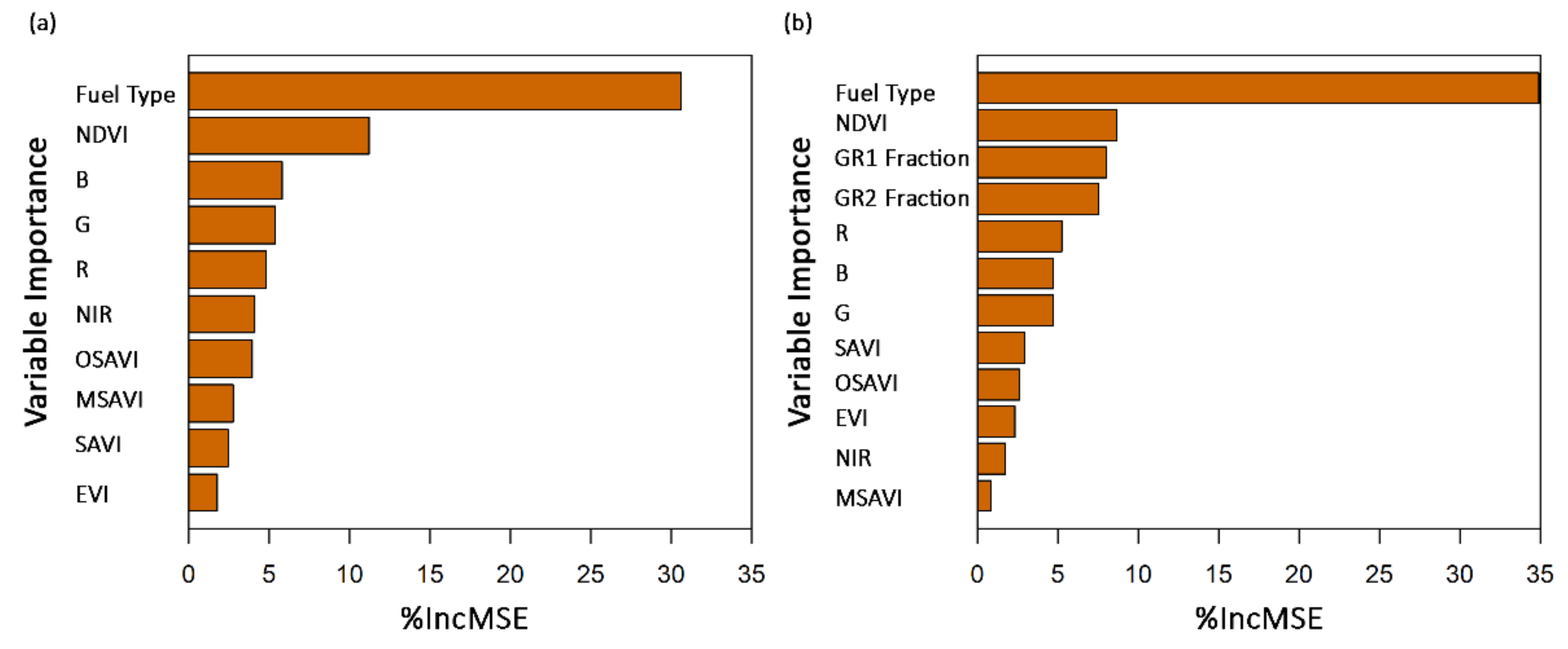
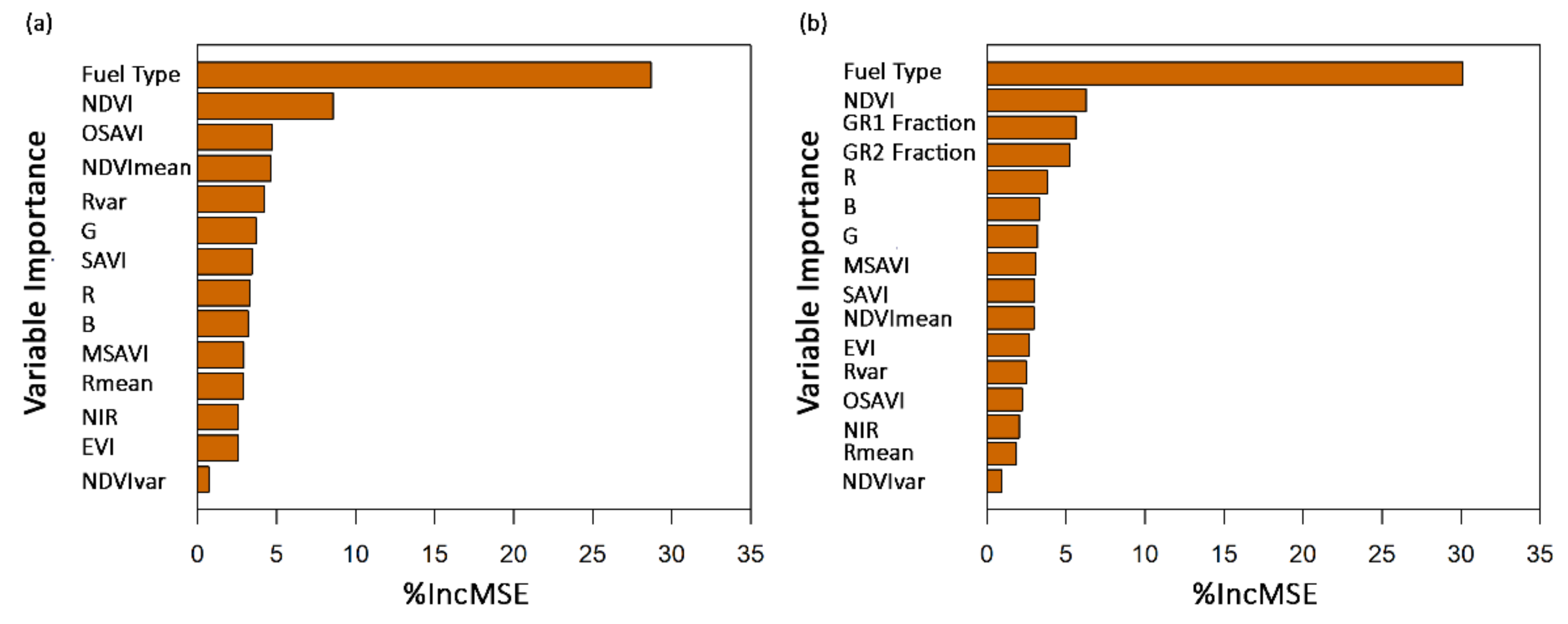
3.2. Comparison of Two Biomass Models Based on Different Input Variables

The first RF model, based on input variables, including the spectral curves from the fuel types, the original spectral bands, and the derived spectral indices, explained 76.20% of the biomass variation with an RMSE of 265.33 kg/ha. The second RF model developed using input variables that included the combination of spectral curves from the fuel types, the original spectral bands, derived vegetation indices, and texture variables, explained 79.80% of the biomass variation with an RMSE of 248.66 kg/ha (Table 4). The inclusion of four texture variables, including the mean and variance of the red band and NDVI in the second RF model, explained an additional 3% of biomass variation. The mapped biomass ranged from 274.38 kg/ha to 2825.74 kg/ha for both models (Table 4; Figure 3). In general, the estimated biomass was higher in the northeast, and lower in the middle parts of the study area (Figure 3a,b). The biomass model that included texture indices as explanatory variables generally had higher biomass values across the majority of the study area than the biomass model without the texture information (Figure 3c).

3.3. Optimal Indices for Estimating Fine Fuel Biomass Based on High Spatial Resolution Images

The contribution of explanatory variables to the overall model performance was evaluated using the %IncMSE test (Figure 4). The %IncMSE value indicates the percentage increase in MSE that occurs when a given variable is included in the model compared to the model without the given variable included. Variable importance indicated that the fuel type had the highest influence on fine fuel biomass estimation for both models. In addition to fuel type, NDVI also had a high influence on biomass estimation (Figure 4). For the model using fuel type, original spectral bands, and vegetation indices as explanatory variables, the inclusion of the red band resulted in a %IncMSE of more than 10%. Other explanatory variables such as MSAVI, SAVI, and NIR had a relatively lower contribution to the model performance (Figure 4a). For the model that included texture indices as explanatory variables, the fuel type, and NDVI, along with the mean texture of the red band, resulted in greater variance explained in the model estimates (Figure 4b).

3.4. Upscaling the Biomass Models Based on Medium Spatial Resolution and Landsat-Derived Spectral Curves

The biomass RF model based on the medium spatial resolution images explained 59.66% of biomass variation (Table 4). The biomass RF model with the combination of fuel type, original spectral bands, and derived vegetation and texture indices as explanatory variables explained 60.07% of the variance in biomass estimation (Table 4). For the biomass RF model based on fuel type, original spectral bands, and vegetation indices as explanatory variables, the inclusion of a fractional cover of GR1 and GR2 fuel types increased the variance explained increased from 59.66% to 64.82%, and decreased RMSE from 218.66 kg/ha to 208.53 kg/ha (Table 4; Figure 5). For the biomass RF model based on fuel type, original spectral bands, and vegetation and texture indicesas explanatory variables, the inclusion of the fuel type fractional cover increased the variance explained from 60.07% to 61.35%, and decreased RMSE from 214.37 kg/ha to 209.94 kg/ha (Table 4). The RF model that included just the fuel type, original spectral bands, and vegetation indices as explanatory variables had biomass that ranged from 291.62 kg/ha to 2491.29 kg/ha (Figure 5a,b) and associated variable importance from this model is shown in Figure 6. For the RF model that used fuel type, original spectral bands, and vegetation and texture indices as explanatory variables, the biomass ranged from 435.64 kg/ha to 2557.89 kg/ha (Table 4; Figure 7a,b). In general, the biomass estimation in pixels for the GR1 fuel type was higher for the RF models that included the texture indices (Figure 5c; Figure 7c).

3.5. Optimal Indices for Fine Fuel Biomass Estimation with Medium Spatial Resolution Images and Landsat Derived Spectral Curves

For the biomass RF model based on the combination of fuel type, original spectral bands, and vegetation indices as explanatory variables, fuel type, and NDVI had higher influences in explaining model variation (Figure 6a). By adding the fractional cover of GR1 and GR2, the model performance improved, and the two variables added ranked third and fourth in variable importance (Figure 6b). For the biomass RF model with fuel type, original spectral bands, and vegetation and texture indices as explanatory variables, the fuel type, and NDVI also had higher influences in explaining model variation, and adding the texture indices contributed to improving the variance explained in biomass estimation (Figure 8a). For the biomass model with fuel type, original spectral bands, vegetation indices, texture indices, and fractional cover as explanatory variables, the fractional cover of GR1 and GR2 ranked third and fourth in improving the model performance (Figure 8b). In general, adding fractional cover increased RF model performance, and adding texture indices as explanatory variables increased the biomass estimation, especially in the GR1 fuel type.
Figure 6. The variable importance for biomass models, based on medium spatial resolution images, (a) without and (b) with fractional cover as explanatory variables. The X-axis is the percent increase in Mean Square Error (%IncMSE). BGfraction and GRfraction are the fractional cover of GR1 and GR2, respectively.
Remotesensing 14 04360 g006
Figure 7. Biomass maps, estimated with the Random Forest algorithm and based on medium spatial resolution images and texture indices: (a) biomass map without fractional cover as explanatory variables, (b) biomass map with fractional cover as explanatory variables, and (c) differences in biomass between the maps with and without fractional cover as explanatory variables.
Remotesensing 14 04360 g007
Figure 8. The variable importance for biomass models based on medium spatial resolution images and texture indices, (a) without and (b) with fractional cover as explanatory variables-. The variable importance for biomass model based on medium spatial resolution images. The X-axis indicated the percent increase in Mean Square Error (%IncMSE). BGfraction and GRfraction indicated the fractional cover of GR1 and GR2, respectively.
Remotesensing 14 04360 g008

4. Discussion

4.1. Estimation and Mapping of Fuel Types

The RF classification of fuel types had high overall accuracy (95%) and appears to capture the heterogeneity in fuel types across the study area (Figure 2). Producer and user accuracy was greater than 89% for all fuel types examined. Tree/shrub fuel types generally had higher misclassification rates (Table 3). At the study site, the Timber-Understory fuel type (TU1) represented clusters of live oak trees having a mixture of small grasses and litter as an understory, or larger mesquite shrubs having subdominant shrubs with litter or small grass/forb understory vegetation. Misclassifications of the TU1 fuel type were likely smaller shrub clusters interspersed with tall grass vegetation. The GS2 fuel type represented individual mesquite or live oak trees with grass understories (typically the cool-season Texas wintergrass or warm-season grasses such as sideoats grama). Misclassifications of this fuel type as GR2 were most likely the result of smaller shrubs having a grass understory comprised of taller grasses. Misclassification of GS2 as TU1 may have been tall individual trees or larger shrubs lacking an herbaceous understory. Peterson et al. [13] reported that shrub fuel models had higher misclassifications because clusters of shrubs can have spectral characteristics similar to closed canopy woodlands and sparse shrubs can have spectral similarities with grassland vegetation, thus increasing the misclassification of this fuel type.

4.2. Estimation Accuracy of Fine Fuel Biomass Based on High Spatial Resolution Images

The fine fuel biomass estimation, based on high spatial resolution images, performed well, with the model explaining more than 80% of the biomass variation. This was consistent with other studies of biomass estimation using high spatial resolution images [23,61]. High spatial resolution images provide a good data source to better estimate heterogeneous biomass and can serve as reliable tools for monitoring rangeland conditions [23,61,62,63]. Additionally, the random forest algorithm proved to be an effective method in predicting herbaceous biomass, consistent with a study by Ramoelo et al. [64]. Several other studies have shown that the random forest algorithm outperformed other approaches in estimating herbaceous biomass [20,65]. For example, the random forest model was superior to models such as partial least squares regression, support vector machines, and back-propagation artificial neural networks for the estimation of grassland biomass in northwest China [20]. RF models were also very robust for estimating herbaceous biomass over large areas such as the Tibetan Plateau and Loess Plateau in China [66,67].

4.3. Importance of Input Variables in Estimating Fine Fuel Biomass

Overall, fuel type and NDVI were important input variables in estimating fine fuel biomass, which was consistent with other studies [27,32,66,67]. Fuel type contributed most to the model prediction and allowed effective separation between relatively high and low biomass [68]. NDVI has been commonly used for predicting biomass production in various ecosystems and performed reasonably well in these studies [69,70,71]. For example, NDVI explained 60% of the variance in herbaceous biomass across 38 sites globally [72]. It was used to estimate forage production in semiarid grasslands across the USA [73], was significantly correlated with biomass in savannas [74], and performed best in estimating grass biomass in the Tallgrass Prairie National Preserve in Kansas [61]. NDVI was a significant variable for predicting aboveground grassland biomass in the Loess Plateau, China [66], and had a high variable importance for predicting biomass of desert steppe in Mongolia and Inner Mongolia [17]. The results of our study also showed that NDVI outperformed other vegetation indices such as MSAVI and SAVI even though these indices were designed to incorporate soil information. Similar results were found in other studies estimating vegetation biomass in arid ecosystems [75,76].
The biomass RF model, based on the combination of the fuel type, original spectral bands, vegetation, and texture indices as explanatory variables, showed a slight improvement in biomass estimation (>81%) compared with the RF model without texture indices as input variables (~77%). Texture indices can identify horizontal structures and spatial variations in images [19,22] which can increase the model’s sensitivity to the spatial characteristics of different fuel types [62], thus contributing to the improvement of model performance. Other studies have suggested the potential of including texture in improving the model performance of biomass estimation, especially based on high spatial resolution images [33,77].

4.4. Performance of Upscaling Biomass Model Based on Medium Spatial Resolution Images

The upscaling of biomass models using the medium spatial resolution images was stable and the addition of fractional cover of fuel types as explanatory variables further improved the model performance. Though the accuracy of the biomass model based on the medium spatial resolution images was lower than that based on the high spatial resolution images, the models remained stable as the influence of input variables was similar to in the models using the high spatial resolution images. The coarser spatial resolution of the medium spatial resolution images may be the main reason for the decrease in RF model accuracy. Each Landsat pixel covered a significantly larger area (900 m2) compared to a pixel of the high spatial resolution images (~0.05 m2). The Landsat pixels also contained heterogeneous ground information and often had mixed herbaceous and woody vegetation types [9] represented in each pixel.
Different from traditional resampling methods [20,78,79], the inclusion of the fractional cover of fuel types in each Landsat pixel along with the spectral curves derived from Landsat images provided a new and more effective way to estimate fine fuel biomass. Adding fractional cover of fuel types as a variable increased the variance explained by the biomass RF model, likely because it was a good indicator of biomass production in grassland ecosystems [79,80]. The variance explained by the RF models using the combination of the fuel type, original spectral bands, vegetation indices, texture indices, and the fractional cover as explanatory variables showed somewhat lower accuracy compared with the model without texture indices. This result suggests that adding more variables may not increase the accuracy of biomass estimation, as additional variables may also increase the uncertainty [11]. The variable importance analysis in RF models using the medium spatial resolution images was similar to those models based on the high spatial resolution images, thus indicating that fuel type and NDVI had stronger influences on biomass estimation.

4.5. Limitations

There are several limitations to this study. First, although the current RF model based on available data achieved relatively high accuracy in biomass estimation, more sampling points distributed throughout the study area could potentially further improve model performance. Second, the relatively long period of field collection and the timing differences between field sampling and remote sensing image acquisition might have, to a degree, increased the uncertainty in biomass estimation. Third, the estimation of the fuel types may introduce some deviations, and the identification of more fuel types would improve the accuracy of the fuel type maps.

5. Conclusions

Rangeland fine fuel biomass is an important variable in fire behavior models and assessments of fine fuel can provide critical information for rangeland management and conservation. This study demonstrated that using high spatial resolution (0.23 m) images and random forest machine learning can effectively map rangeland fine fuel biomass with relatively high accuracy (>80%), using the spectral curves from visible and NIR bands as well as vegetation and texture indices derived from these bands as input variables in the biomass RF models. Accounting for the influences of texture in the model increased the accuracy of biomass estimation from 76% to 80%. The biomass RF models derived from high-resolution images were also upscaled to a medium spatial resolution (30 m) to examine the RF model stability and performance. The results showed that the fuel type and NDVI were significant input variables influencing rangeland fine fuel biomass estimations with both high and medium spatial resolution remote sensing images. The addition of a fractional cover of the different fuel types helped improve the accuracy of biomass estimates derived from moderate-resolution imagery (Landsat). These findings contribute to our understanding of biomass estimation using machine learning algorithms with remote sensing images of different spatial resolutions. This study is an important step towards developing models that can effectively estimate rangeland fine fuel biomass with high accuracy over large regions using commonly available remote sensing data, which is essential for the management and planning efforts related to both prescribed fire and wildfires on rangelands from landscape to regional scales. Furthermore, the ability to map fuel type and fuel amounts could be useful for modeling fire spread and assessing fuel conditions that could lead to high burn severity or damage to sensitive vegetation communities.

Author Contributions

Conceptualization, Z.L., J.P.A. and X.B.W.; Methodology, Z.L., J.P.A., X.B.W., X.J. and C.Y.; Formal analysis, Z.L.; Investigation, Z.L., J.P.A. and X.B.W.; Data curation, Z.L., X.J. and C.Y.; Writing—original draft preparation, Z.L.; Writing—review and editing, Z.L., J.P.A., X.B.W. and C.Y.; Funding acquisition, X.B.W. and J.P.A. All authors have read and agreed to the published version of the manuscript.

Funding

This research was supported in part by the U.S. Department of Agriculture’s Agriculture Research Service and the National Institute of Food and Agriculture (2019-68012-29819 and Hatch Project 1003961). The U.S. Department of Agriculture is an equal opportunity lender, provider, and employer. Support was also provided to Zheng Li through a Tom Slick Graduate Research Fellowship from the College of Agriculture and Life Sciences, Texas A&M University.

Data Availability Statement

Not applicable.

Acknowledgments

We thank Jesse Goplin, Deann Burson, Jose Mata, and Weiqian Gao for their assistance in field data collection, John Walker and Doug Tolleson for their advice and logistical support for the field work, and Sam Fuhlendorf for the helpful discussions related to this study.

Conflicts of Interest

The authors declare no conflict of interest.

References

  1. Estell, R.E.; Havstad, K.M.; Cibils, A.F.; Fredrickson, E.L.; Anderson, D.M.; Schrader, T.; James, D.K. Increasing shrub use by livestock in a world with less grass. Rangel. Ecol. Manag. 2012, 65, 553–562. [Google Scholar] [CrossRef]
  2. Havstad, K.M.; Peters, D.P.; Skaggs, R.; Brown, J.; Bestelmeyer, B.; Fredrickson, E.; Herrick, J.; Wright, J. Ecological services to and from rangelands of the United States. Ecol. Econ. 2007, 64, 261–268. [Google Scholar] [CrossRef]
  3. Havstad, K.; Peters, D.; Allen-Diaz, B.; Bartolome, J.; Herrick, J.; Huntsinger, L.; Johnson, P.; Joyce, L. Rangelands: A Major Resource. Grassland: Quietness and Strength for a New American Agriculture; ASA-CSSA-SSSA: Madison, WI, USA, 2009; Volume 142, p. 75. [Google Scholar]
  4. Yahdjian, L.; Sala, O.E.; Havstad, K.M. Rangeland ecosystem services: Shifting focus from supply to reconciling supply and demand. Front. Ecol. Environ. 2015, 13, 44–51. [Google Scholar] [CrossRef]
  5. Sala, O.E.; Paruelo, J.M. Ecosystem services in grasslands. In Nature’s Services: Societal Dependence on Natural Ecosystems; Island Press: Washington, DC, USA, 1997; pp. 237–251. [Google Scholar]
  6. Twidwell, D.; Bielski, C.H.; Scholtz, R.; Fuhlendorf, S.D. Advancing fire ecology in 21st century rangelands. Rangel. Ecol. Manag. 2021, 78, 201–212. [Google Scholar] [CrossRef]
  7. Li, Z.; Angerer, J.; Wu, X.B. The impacts of wildfires of different burn severities on vegetation structure across the western United States rangelands. Sci. Total Environ. 2022, 845, 157214. [Google Scholar] [CrossRef]
  8. Fuhlendorf, S.D.; Fynn, R.W.; McGranahan, D.A.; Twidwell, D. Heterogeneity as the basis for rangeland management. In Rangeland Systems; Springer: Cham, Switzerland, 2017; pp. 169–196. [Google Scholar] [CrossRef]
  9. Kong, B.; Yu, H.; Du, R.; Wang, Q. Quantitative estimation of biomass of alpine grasslands using hyperspectral remote sensing. Rangel. Ecol. Manag. 2019, 72, 336–346. [Google Scholar] [CrossRef]
  10. Chen, J.; Gu, S.; Shen, M.; Tang, Y.; Matsushita, B. Estimating aboveground biomass of grassland having a high canopy cover: An exploratory analysis of in situ hyperspectral data. Int. J. Remote Sens. 2009, 30, 6497–6517. [Google Scholar] [CrossRef]
  11. Sesnie, S.E.; Eagleston, H.; Johnson, L.; Yurcich, E. In-situ and remote sensing platforms for mapping fine-fuels and fuel-types in Sonoran semi-desert grasslands. Remote Sens. 2018, 10, 1358. [Google Scholar] [CrossRef]
  12. Huff, S.; Poudel, K.P.; Ritchie, M.; Temesgen, H. Quantifying aboveground biomass for common shrubs in northeastern California using nonlinear mixed effect models. For. Ecol. Manag. 2018, 424, 154–163. [Google Scholar] [CrossRef]
  13. Peterson, S.H.; Franklin, J.; Roberts, D.A.; van Wagtendonk, J.W. Mapping fuels in Yosemite National Park. Can. J. For. Res. 2012, 43, 7–17. [Google Scholar] [CrossRef]
  14. Barrachina, M.; Cristóbal, J.; Tulla, A.F. Estimating above-ground biomass on mountain meadows and pastures through remote sensing. Int. J. Appl. Earth Obs. Geoinf. 2015, 38, 184–192. [Google Scholar] [CrossRef]
  15. Pham, L.T.; Brabyn, L. Monitoring mangrove biomass change in Vietnam using SPOT images and an object-based approach combined with machine learning algorithms. ISPRS J. Photogramm. Remote Sens. 2017, 128, 86–97. [Google Scholar] [CrossRef]
  16. Fern, R.R.; Foxley, E.A.; Bruno, A.; Morrison, M.L. Suitability of NDVI and OSAVI as estimators of green biomass and coverage in a semi-arid rangeland. Ecol. Indic. 2018, 94, 16–21. [Google Scholar] [CrossRef]
  17. John, R.; Chen, J.; Giannico, V.; Park, H.; Xiao, J.; Shirkey, G.; Ouyang, Z.; Shao, C.; Lafortezza, R.; Qi, J. Grassland canopy cover and aboveground biomass in Mongolia and Inner Mongolia: Spatiotemporal estimates and controlling factors. Remote Sens. Environ. 2018, 213, 34–48. [Google Scholar] [CrossRef]
  18. Otgonbayar, M.; Atzberger, C.; Chambers, J.; Damdinsuren, A. Mapping pasture biomass in Mongolia using partial least squares, random forest regression and Landsat 8 imagery. Int. J. Remote Sens. 2019, 40, 3204–3226. [Google Scholar] [CrossRef]
  19. Li, C.; Zhou, L.; Xu, W. Estimating aboveground biomass using Sentinel-2 MSI data and ensemble algorithms for grassland in the Shengjin Lake Wetland, China. Remote Sens. 2021, 13, 1595. [Google Scholar] [CrossRef]
  20. Tang, R.; Zhao, Y.; Lin, H. Spatio-temporal variation characteristics of aboveground biomass in the headwater of the yellow river based on machine learning. Remote Sens. 2021, 13, 3404. [Google Scholar] [CrossRef]
  21. Wang, J.; Xiao, X.; Bajgain, R.; Starks, P.; Steiner, J.; Doughty, R.B.; Chang, Q. Estimating leaf area index and aboveground biomass of grazing pastures using Sentinel-1, Sentinel-2 and Landsat images. ISPRS J. Photogramm. Remote Sens. 2019, 154, 189–201. [Google Scholar] [CrossRef]
  22. Tian, Y.; Huang, H.; Zhou, G.; Zhang, Q.; Tao, J.; Zhang, Y.; Lin, J. Aboveground mangrove biomass estimation in Beibu Gulf using machine learning and UAV remote sensing. Sci. Total Environ. 2021, 781, 146816. [Google Scholar] [CrossRef]
  23. Pecina, M.V.; Bergamo, T.F.; Ward, R.; Joyce, C.; Sepp, K. A novel UAV-based approach for biomass prediction and grassland structure assessment in coastal meadows. Ecol. Indic. 2021, 122, 107227. [Google Scholar] [CrossRef]
  24. Ullah, S.; Si, Y.; Schlerf, M.; Skidmore, A.K.; Shafique, M.; Iqbal, I.A. Estimation of grassland biomass and nitrogen using MERIS data. Int. J. Appl. Earth Obs. Geoinf. 2012, 19, 196–204. [Google Scholar] [CrossRef]
  25. Zhao, F.; Xu, B.; Yang, X.; Jin, Y.; Li, J.; Xia, L.; Chen, S.; Ma, H. Remote sensing estimates of grassland aboveground biomass based on MODIS net primary productivity (NPP): A case study in the Xilingol grassland of Northern China. Remote Sens. 2014, 6, 5368–5386. [Google Scholar] [CrossRef]
  26. Tucker, C.J. Red and photographic infrared linear combinations for monitoring vegetation. Remote Sens. Environ. 1979, 8, 127–150. [Google Scholar] [CrossRef]
  27. Yang, S.; Feng, Q.; Liang, T.; Liu, B.; Zhang, W.; Xie, H. Modeling grassland above-ground biomass based on artificial neural network and remote sensing in the Three-River Headwaters Region. Remote Sens. Environ. 2018, 204, 448–455. [Google Scholar] [CrossRef]
  28. Steven, M.D. The sensitivity of the OSAVI vegetation index to observational parameters. Remote Sens. Environ. 1998, 63, 49–60. [Google Scholar] [CrossRef]
  29. Huete, A.; Justice, C.; Liu, H. Development of vegetation and soil indices for MODIS-EOS. Remote Sens. Environ. 1994, 49, 224–234. [Google Scholar] [CrossRef]
  30. Huete, A.R. A soil-adjusted vegetation index (SAVI). Remote Sens. Environ. 1988, 25, 295–309. [Google Scholar] [CrossRef]
  31. Qi, J.; Chehbouni, A.; Huete, A.; Kerr, Y.; Sorooshian, S. A modified soil adjusted vegetation index. Remote Sens. Environ. 1994, 48, 119–126. [Google Scholar] [CrossRef]
  32. Liang, T.; Yang, S.; Feng, Q.; Liu, B.; Zhang, R.; Huang, X.; Xie, H. Multi-factor modeling of above-ground biomass in alpine grassland: A case study in the Three-River Headwaters Region, China. Remote Sens. Environ. 2016, 186, 164–172. [Google Scholar] [CrossRef]
  33. Poley, G.L.; McDermid, J.G. A systematic review of the factors influencing the estimation of vegetation aboveground biomass using unmanned aerial systems. Remote Sens. 2020, 12, 1052. [Google Scholar] [CrossRef]
  34. Kelsey, K.C.; Neff, J.C. Estimates of aboveground biomass from texture analysis of Landsat imagery. Remote Sens. 2014, 6, 6407–6422. [Google Scholar] [CrossRef]
  35. Sarker, L.R.; Nichol, J.E. Improved forest biomass estimates using ALOS AVNIR-2 texture indices. Remote Sens. Environ. 2011, 115, 968–977. [Google Scholar] [CrossRef]
  36. Wallis, C.I.; Homeier, J.; Peña, J.; Brandl, R.; Farwig, N.; Bendix, J. Modeling tropical montane forest biomass, productivity and canopy traits with multispectral remote sensing data. Remote Sens. Environ. 2019, 225, 77–92. [Google Scholar] [CrossRef]
  37. Zhang, C.; Denka, S.; Cooper, H.; Mishra, D.R. Quantification of sawgrass marsh aboveground biomass in the coastal Everglades using object-based ensemble analysis and Landsat data. Remote Sens. Environ. 2018, 204, 366–379. [Google Scholar] [CrossRef]
  38. Wang, L.A.; Zhou, X.; Zhu, X.; Dong, Z.; Guo, W. Estimation of biomass in wheat using random forest regression algorithm and remote sensing data. Crop J. 2016, 4, 212–219. [Google Scholar] [CrossRef]
  39. Gleason, C.J.; Im, J. Forest biomass estimation from airborne LiDAR data using machine learning approaches. Remote Sens. Environ. 2012, 125, 80–91. [Google Scholar] [CrossRef]
  40. Forkuor, G.; Zoungrana, J.-B.B.; Dimobe, K.; Ouattara, B.; Vadrevu, K.P.; Tondoh, J.E. Above-ground biomass mapping in West African dryland forest using Sentinel-1 and 2 datasets-A case study. Remote Sens. Environ. 2020, 236, 111496. [Google Scholar] [CrossRef]
  41. Chen, L.; Ren, C.; Zhang, B.; Wang, Z.; Xi, Y. Estimation of forest above-ground biomass by geographically weighted regression and machine learning with sentinel imagery. Forests 2018, 9, 582. [Google Scholar] [CrossRef]
  42. Daly, C.; Halbleib, M.; Smith, J.I.; Gibson, W.P.; Doggett, M.K.; Taylor, G.H.; Curtis, J.; Pasteris, P.P. Physiographically sensitive mapping of climatological temperature and precipitation across the conterminous United States. Int. J. Climatol. 2008, 28, 2031–2064. [Google Scholar] [CrossRef]
  43. NRCS, Natural Resources Conservation Service, United States Department of Agriculture. Web Soil Survey. Available online: http://www.Websoilsurvey.ncsc.usda.gov (accessed on 21 February 2022).
  44. Elliott, L.F.; Diamond, D.D.; True, C.D.; Blodgett, C.F.; Pursell, D.; German, D.; Treuer-Kuehn, A. Ecological Mapping Systems of Texas: Summary Report; Texas Parks and Wildlife Department: Austin, TX, USA, 2014.
  45. McGinty, A.; Smeins, F.E.; Merrill, L.B. Influence of spring burning on cattle diets and performance on the Edwards Plateau. Rangel. Ecol. Manag. 1983, 36, 175–178. [Google Scholar] [CrossRef]
  46. Scott, J.H.; Burgan, R.E. Standard Fire Behavior Fuel Models: A Comprehensive Set for Use with Rothermel’s Surface Fire Spread Model; Gen. Tech. Rep. RMRS-GTR-153; US Department of Agriculture, Forest Service, Rocky Mountain Research Station: Fort Collins, CO, USA, 2005. [CrossRef]
  47. Roy, D.P.; Wulder, M.A.; Loveland, T.R.; Woodcock, C.E.; Allen, R.G.; Anderson, M.C.; Helder, D.; Irons, J.R.; Johnson, D.M.; Kennedy, R. Landsat-8: Science and product vision for terrestrial global change research. Remote Sens. Environ. 2014, 145, 154–172. [Google Scholar] [CrossRef]
  48. Guerini Filho, M.; Kuplich, T.M.; Quadros, F.L.D. Estimating natural grassland biomass by vegetation indices using Sentinel 2 remote sensing data. Int. J. Remote Sens. 2020, 41, 2861–2876. [Google Scholar] [CrossRef]
  49. Jin, Y.; Yang, X.; Qiu, J.; Li, J.; Gao, T.; Wu, Q.; Zhao, F.; Ma, H.; Yu, H.; Xu, B. Remote sensing-based biomass estimation and its spatio-temporal variations in temperate grassland, Northern China. Remote Sens. 2014, 6, 1496–1513. [Google Scholar] [CrossRef]
  50. Zhou, Y.; Zhang, L.; Xiao, J.; Chen, S.; Kato, T.; Zhou, G. A comparison of satellite-derived vegetation indices for approximating gross primary productivity of grasslands. Rangel. Ecol. Manag. 2014, 67, 9–18. [Google Scholar] [CrossRef]
  51. Ren, H.; Zhou, G.; Zhang, X. Estimation of green aboveground biomass of desert steppe in Inner Mongolia based on red-edge reflectance curve area method. Biosyst. Eng. 2011, 109, 385–395. [Google Scholar] [CrossRef]
  52. Haralick, R.M.; Shanmugam, K.; Dinstein, I.H. Textural features for image classification. IEEE Trans. Syst. Man Cybern. 1973, 6, 610–621. [Google Scholar] [CrossRef]
  53. Rouse, J.W.; Haas, R.H.; Schell, J.A.; Deering, D.W. Monitoring the vernal advancement and retrogradation (greenwave effect) of natural vegetation. NASA Goddard Sp. Flight Cent. 1974, 351, 309. [Google Scholar]
  54. Jiang, Z.; Huete, A.R.; Didan, K.; Miura, T. Development of a two-band enhanced vegetation index without a blue band. Remote Sens. Environ. 2008, 112, 3833–3845. [Google Scholar] [CrossRef]
  55. Rondeaux, G.; Steven, M.; Baret, F. Optimization of soil-adjusted vegetation indices. Remote Sens. Environ. 1996, 55, 95–107. [Google Scholar] [CrossRef]
  56. Breiman, L. Random forests. Mach. Learn. 2001, 45, 5–32. [Google Scholar] [CrossRef]
  57. Amatulli, G.; Camia, A.; San-Miguel-Ayanz, J.J. Estimating future burned areas under changing climate in the EU-Mediterranean countries. Sci. Total Environ. 2013, 450, 209–222. [Google Scholar] [CrossRef]
  58. Dillon, G.K.; Holden, Z.A.; Morgan, P.; Crimmins, M.A.; Heyerdahl, E.K.; Luce, C.H. Both topography and climate affected forest and woodland burn severity in two regions of the western US, 1984–2006. Ecosphere 2011, 2, 1–33. [Google Scholar] [CrossRef]
  59. Robinson, N.P.; Jones, M.O.; Moreno, A.; Erickson, T.A.; Naugle, D.E.; Allred, B.W. Rangeland productivity partitioned to sub-pixel plant functional types. Remote Sens. 2019, 11, 1427. [Google Scholar] [CrossRef]
  60. R Core Team. R: A Language and Environment for Statistical Computing; R Core Team: Vienna, Austria, 2013. [Google Scholar]
  61. Wang, H.; Wang, C.; Price, K.P.; van der Merwe, D.; An, N. Modeling above-ground biomass in tallgrass prairie using ultra-high spatial resolution sUAS imagery. Photogramm. Eng. Remote Sens. 2014, 80, 1151–1159. [Google Scholar] [CrossRef]
  62. Sibanda, M.; Mutanga, O.; Rouget, M.; Kumar, L. Estimating biomass of native grass grown under complex management treatments using worldview-3 spectral derivatives. Remote Sens. 2017, 9, 55. [Google Scholar] [CrossRef]
  63. Michez, A.; Lejeune, P.; Bauwens, S.; Herinaina, A.A.L.; Blaise, Y.; Castro Muñoz, E.; Lebeau, F.; Bindelle, J. Mapping and monitoring of biomass and grazing in pasture with an unmanned aerial system. Remote Sens. 2019, 11, 473. [Google Scholar] [CrossRef]
  64. Ramoelo, A.; Cho, M.A.; Mathieu, R.; Madonsela, S.; Van De Kerchove, R.; Kaszta, Z.; Wolff, E. Monitoring grass nutrients and biomass as indicators of rangeland quality and quantity using random forest modelling and WorldView-2 data. Int. J. Appl. Earth Obs. Geoinf. 2015, 43, 43–54. [Google Scholar] [CrossRef]
  65. Zeng, N.; Ren, X.; He, H.; Zhang, L.; Zhao, D.; Ge, R.; Li, P.; Niu, Z. Estimating grassland aboveground biomass on the Tibetan Plateau using a random forest algorithm. Ecol. Indic. 2019, 102, 479–487. [Google Scholar] [CrossRef]
  66. Wang, Y.; Wu, G.; Deng, L.; Tang, Z.; Wang, K.; Sun, W.; Shangguan, Z. Prediction of aboveground grassland biomass on the Loess Plateau, China, using a random forest algorithm. Sci. Rep. 2017, 7, 6940. [Google Scholar] [CrossRef] [PubMed] [Green Version]
  67. Xia, J.; Ma, M.; Liang, T.; Wu, C.; Yang, Y.; Zhang, L.; Zhang, Y.; Yuan, W. Estimates of grassland biomass and turnover time on the Tibetan Plateau. Environ. Res. Lett. 2018, 13, 014020. [Google Scholar] [CrossRef]
  68. Avitabile, V.; Baccini, A.; Friedl, M.A.; Schmullius, C. Capabilities and limitations of Landsat and land cover data for aboveground woody biomass estimation of Uganda. Remote Sens. Environ. 2012, 117, 366–380. [Google Scholar] [CrossRef]
  69. Tucker, C.J.; Justice, C.; Prince, S. Monitoring the grasslands of the Sahel 1984–1985. Int. J. Remote Sens. 1986, 7, 1571–1581. [Google Scholar] [CrossRef]
  70. Rigge, M.; Smart, A.; Wylie, B.; Gilmanov, T.; Johnson, P. Linking phenology and biomass productivity in South Dakota mixed-grass prairie. Rangel. Ecol. Manag. 2013, 66, 579–587. [Google Scholar] [CrossRef]
  71. Xie, Y.; Sha, Z.; Yu, M.; Bai, Y.; Zhang, L. A comparison of two models with Landsat data for estimating above ground grassland biomass in Inner Mongolia, China. Ecol. Modell. 2009, 220, 1810–1818. [Google Scholar] [CrossRef]
  72. Xia, J.; Liu, S.; Liang, S.; Chen, Y.; Xu, W.; Yuan, W. Spatio-temporal patterns and climate variables controlling of biomass carbon stock of global grassland ecosystems from 1982 to 2006. Remote Sens. 2014, 6, 1783–1802. [Google Scholar] [CrossRef]
  73. Poděbradská, M.; Wylie, B.K.; Bathke, D.J.; Bayissa, Y.A.; Dahal, D.; Derner, J.D.; Fay, P.A.; Hayes, M.J.; Schacht, W.H.; Volesky, J.D. Monitoring climate impacts on annual forage production across US semi-arid grasslands. Remote Sens. 2022, 14, 4. [Google Scholar] [CrossRef]
  74. Chapungu, L.; Nhamo, L.; Gatti, R.C. Estimating biomass of savanna grasslands as a proxy of carbon stock using multispectral remote sensing. Remote Sens. Appl. Soc. Environ. 2020, 17, 100275. [Google Scholar] [CrossRef]
  75. Franklin, J.; Duncan, J.; Turner, D.L. Reflectance of vegetation and soil in Chihuahuan desert plant communities from ground radiometry using SPOT wavebands. Remote Sens. Environ. 1993, 46, 291–304. [Google Scholar] [CrossRef]
  76. McGwire, K.; Minor, T.; Fenstermaker, L. Hyperspectral mixture modeling for quantifying sparse vegetation cover in arid environments. Remote Sens. Environ. 2000, 72, 360–374. [Google Scholar] [CrossRef]
  77. Ploton, P.; Barbier, N.; Couteron, P.; Antin, C.; Ayyappan, N.; Balachandran, N.; Barathan, N.; Bastin, J.-F.; Chuyong, G.; Dauby, G. Toward a general tropical forest biomass prediction model from very high resolution optical satellite images. Remote Sens. Environ. 2017, 200, 140–153. [Google Scholar] [CrossRef]
  78. Fassnacht, F.E.; Poblete-Olivares, J.; Rivero, L.; Lopatin, J.; Ceballos-Comisso, A.; Galleguillos, M. Using Sentinel-2 and canopy height models to derive a landscape-level biomass map covering multiple vegetation types. Int. J. Appl. Earth Obs. Geoinf. 2021, 94, 102236. [Google Scholar] [CrossRef]
  79. Yu, R.; Yao, Y.; Wang, Q.; Wan, H.; Xie, Z.; Tang, W.; Zhang, Z.; Yang, J.; Shang, K.; Guo, X. Satellite-derived estimation of grassland aboveground biomass in the Three-River Headwaters Region of China during 1982–2018. Remote Sens. 2021, 13, 2993. [Google Scholar] [CrossRef]
  80. Lehnert, L.W.; Meyer, H.; Wang, Y.; Miehe, G.; Thies, B.; Reudenbach, C.; Bendix, J. Retrieval of grassland plant coverage on the Tibetan Plateau based on a multi-scale, multi-sensor and multi-method approach. Remote Sens. Environ. 2015, 164, 197–207. [Google Scholar] [CrossRef]
Figure 2. The classification map of fuel types for the study area. GR1 and GR2 represent Grass Fuel Type Models, GS2 represents Grass-Shrub Fuel Type Model, and TU1 represents Timber-Understory Fuel Type Model.
Remotesensing 14 04360 g002
Figure 3. Biomass maps based on high spatial resolution images: (a) biomass map without texture indices as explanatory variables, (b) biomass map with texture indices as explanatory variables, and (c) differences between the biomass maps with and without texture indices as explanatory variables.
Remotesensing 14 04360 g003
Figure 4. The variable importance for biomass model based on high spatial resolution images. (a) the variable importance for the biomass model without texture indices as explanatory variables based on the high spatial resolution images, (b) the variable importance for the model with texture indices as explanatory variables based on the high spatial resolution images. The X-axis indicates the percent increase in Mean Square Error (%IncMSE). B, G, R, and NIR represent the spectral curves for blue, green, red, and near-infrared bands of the high-resolution imagery, respectively. Rmean, Rvar, NDVImean, and NDVIvar represent the mean and variance of the texture calculations on the red band and NDVI, respectively.
Remotesensing 14 04360 g004
Figure 5. Biomass maps based on medium spatial resolution images: (a) biomass map without fractional cover as explanatory variables, (b) biomass map with fractional cover as explanatory variables, and (c) the differences in biomass between the maps with and without fractional cover as explanatory variables.
Remotesensing 14 04360 g005
Table 1. The selected fuel types from the Scott and Burgan Fire Behavior Model [46].
NameDescription
Grass Fuel Type Model (GR1)The primary carrier of fire in GR1 is sparse grass and the grass in GR1 is generally short.
Grass Fuel Type Model (GR2)The primary carrier of fire in GR2 is grass and the fuel load is greater than GR1.
Grass-Shrub Fuel Type Model (GS2)The primary carrier of fire in GS2 is grass and shrub combined. Shrubs are 1 to 3 feet high. Grass load is moderate.
Timber-Understory Fuel Type Model (TU1)The primary carrier of fire in TU1 is low load of grass and/or shrub with litter.
Table 2. The vegetation and texture indices for estimation of fine fuel biomass using the random forest algorithm.
CategoryIndicesEquationReferences
VegetationNormalized Difference Vegetation Index (NDVI)(NIR − R)/(NIR + R)[53]
Soil Adjusted Vegetation Index (SAVI)((NIR − R)/(NIR + R + 0.5)) × 1.5[30]
Modified Soil Adjusted Vegetation Index (MSAVI)(2 × NIR + 1 − SQRT((2 × NIR + 1)2 − 8 × (NIR − R)))/2[31]
Enhanced Vegetation Index (EVI)2.5 × ((NIR − R)/(NIR + 6 × R − 7.5 × B + 1))[54]
Optimized Soil Adjusted Vegetation Index (OSAVI)(NIR − R)/(NIR + R + 0.16)[55]
Mean (MEA) i , j = 0 N 1 i P i j [52]
TextureVariance (VAR) i , j = 0 N 1 P i , j 1 µ i 2 [52]
Table 3. Classification error matrix for fuel type classification.
Reference Data
GR1GR2TU1ShadowGS2User’s Accuracy (%)
Classified dataGR114521100099.25
GR2101490002897.51
TU1001387012991.49
Shadow0121448799.31
GS20251247136189.72
Producer’s Accuracy (%)99.3297.5891.6799.5289.25
Table 4. The results of the random forest (RF) models used for fine fuel biomass estimation (kg/ha) based on different explanatory variables and different spatial resolution images. The mtry parameter represents the number of randomly selected predictors at each node in the RF analysis. The ntree parameter, which represents the number of trees grown in the model, was set to 500 for all models listed below.
Spatial ResolutionInput VariablesNo. of VariablesMtry ParameterVariance ExplainedMAERMSE
Highfuel type,
original spectral bands and vegetation indices
10376.20%226.54265.33
fuel type,
original spectral bands, vegetation indices, and texture indices
14479.80%212.53248.66
Mediumfuel type,
original spectral bands and vegetation indices
10359.66%162.19218.66
fuel type,
original spectral bands, vegetation indices, and fractional cover
12464.82%154.63208.53
fuel type,
original spectral bands, vegetation indices, and texture indices
14460.07%162.44214.37
fuel type,
original spectral bands, vegetation indices, texture indices, and fractional cover
16561.35%163.82209.94
Publisher’s Note: MDPI stays neutral with regard to jurisdictional claims in published maps and institutional affiliations.

