A Novel Historical Landslide Detection Approach Based on LiDAR and Lightweight Attention U-Net

Abstract

Rapid and accurate identification of landslides is an essential part of landslide hazard assessment, and in particular it is useful for land use planning, disaster prevention, and risk control. Recent alternatives to manual landslide mapping are moving in the direction of artificial intelligence—aided recognition of these surface processes. However, so far, the technological advancements have not produced robust automated mapping tools whose domain of validity holds in any area across the globe. For instance, capturing historical landslides in densely vegetated areas is still a challenge. This study proposed a deep learning method based on Light Detection and Ranging (LiDAR) data for automatic identification of historical landslides. Additionally, it tested this method in the Jiuzhaigou earthquake-hit region of Sichuan Province (China). Specifically, we generated a Red Relief Image Map (RRIM), which was obtained via high-precision airborne LiDAR data, and on the basis of this information we trained a Lightweight Attention U-Net (LAU-Net) to map a total of 1949 historical landslides. Overall, our model recognized the aforementioned landslides with high accuracy and relatively low computational costs. We compared multiple performance indexes across several deep learning routines and different data types. The results showed that the Multiple-Class based Semantic Image Segmentation (MIOU) and the F1_score of the LAU-Net and RRIM reached 82.29% and 87.45%, which represented the best performance among the methods we tested.

1. Introduction

Landslides pose severe threats to human lives, activities, and infrastructure in mountainous terrains [1,2,3]. Understanding their genesis and dynamics is fundamental to reduce landslide risks [4,5]. In this context, record and monitoring data help gain insights on how landslides behave. The way the geoscientific community gathering landslide records fundamentally boils down to landslide identification routines. These have originally been based on field surveys and expert-based landslide recognition practices using orthophotos or satellite scenes [6]. However, such practices suffer from a high degree of subjectivity, and they also require a significant amount of time and resources [7]. Conversely, more recent technological advancements have pointed out the use of automated landslide recognition to standardize the procedure towards objective results produced with a significant speed-up [8].

Among the automated landslide mapping procedures proposed so far, the selection of the data and the algorithmic architecture one may use imply some limitations [9,10,11,12]. For instance, the choice of optical images brings a clear and interpretable overview of an area unless affected by cloud and/or dense vegetation covers [13,14,15,16]. Conversely, radar images are less sensitive to these issues, although the signal they record is a function of surface deformation data [17,18]. Therefore, these images may not be suitable to map historical landslides. In this context, Light Detection and Ranging (LiDAR) may prove to be crucial in bringing a third and complementary type of information compared to the two data sources mentioned above. LiDAR technology has gradually gained the spotlight in recent years to identify any sort of geological hazards in mountainous areas [19,20,21,22,23,24]. In fact, compared with conventional optical image, the use of LiDAR carries several advantages. It provides high resolution topographic data, enabling detailed analysis of geomorphic features and surface deformation. It also allows one to remove the influence of vegetation [20,25,26]. However, the use of LiDAR for landslide identification has yet to become prominent compared to the optic and radar counterparts. Specifically, most of its uses are still based on manual interpretation on morphometric properties derived from the LiDAR survey [27,28]. However, methodologically, the geoscientific community has reached a level of maturity where artificial intelligence may replace manual efforts, with the only confusion brought by the numerous alternatives available to take on this task. Several examples exist in fact where researchers have used different machine learning algorithms such as Artificial Neural Network, Random Forest, and Support vector machine to draw landslide maps [29,30,31,32,33,34,35]. However, these tools generally suffered from inaccuracies, resulting in large numbers of false positives [36,37]. Even more recently, the above-mentioned routines have mostly been superseded by deep learning approaches specifically because of their enhanced precision, with examples of striking accuracies associated with relatively low FPs [35]. Specifically, Convolutional Neural Network (CNN), Channel Attention CNN, GAN-based Siamese framework, and Region Convolutional Neural Network have made remarkable progress in landslides recognition based on optical image [17,36,38,39,40,41,42,43,44]. In this broad context, deep learning routines coupled with LiDAR data are yet to be fully explored, especially for mapping historical landslides.

This paper attempts to fill this gap, by proposing a new automatic landslides identification method based on LiDAR data, whose information is passed to a series of deep learning routines to retrieve historical landslide signatures in a test site located within the Jiuzhaigou region of Sichuan Province (China).

2. Study Area and Data

2.1. Study Area

The study site we selected is located within the Jiuzhaigou, Aba Tibetan Autonomous Prefecture of Sichuan Province, and it covers an area of approximately 356.73 km² (Figure 1).

The study area is almost completely contained within the Jiuzhaigou National Forest Park, characterized by a subtropical monsoon climate responsible for an average annual rainfall of about 500–600 mm [45]. The altitude ranges from 1892 to 4359 above mean sea level, and the underlying lithology mostly consists of bioclastic limestone and calcareous dolomite, at times featuring deep canyon landform [46].

Historically, a number of geological disasters have taken place within the area. The Jiuzhaigou earthquake on 8 August 2017 is certainly the most recent one [47]. However, several other earthquakes have been reported in the literature through the years. However, a comprehensive historical landslide inventory has not been compiled so far, and the public information on past slope failures has mainly been achieved through simulations [48]. One of the reasons behind this is due to the vegetation, which covers approximately 79.4% of the study area [49].

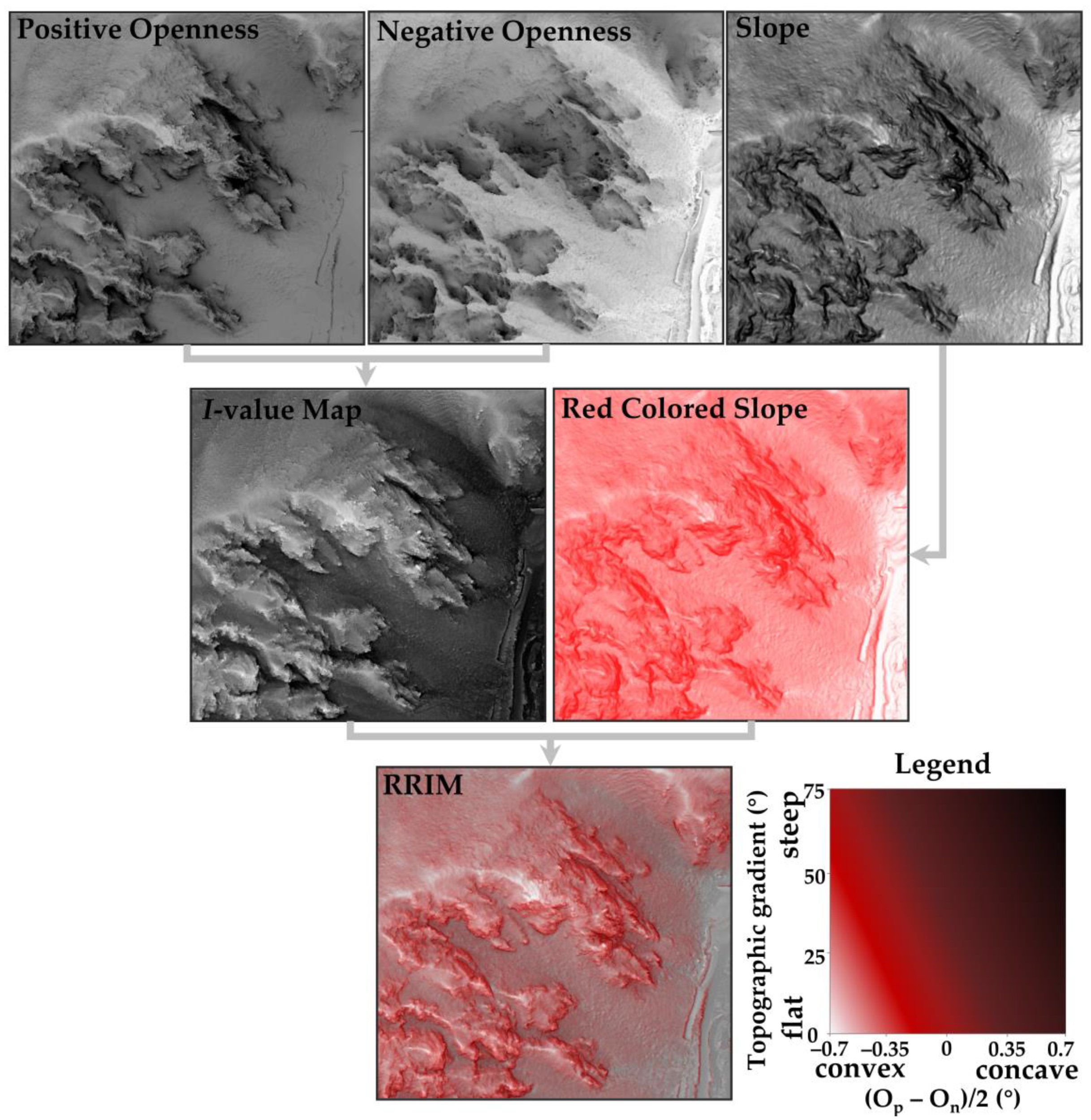
2.2. Data Preparation

The airborne LiDAR data was initially used to obtain the point cloud (provided by Sichuan Bureau of Surveying and Mapping (SBSM), and the point cloud density is 30 pints/m²) from Wuhuahai to Rizegou, and these locations were hit by the earthquake in 2017. Because the obtained point cloud data removed vegetation and buildings, we generated DEM of this region by © ArcGIS Pro. Firstly, the LAS dataset was created by using data management tools. Subsequently, the LAS dataset was converted to a 1 m resolution DEM. In the conversion process, the interpolation type was selected by natural neighbor method, and the sampling value was set as 1. At the same time, we also obtained the same range of UAV optical images (0.2 m × 0.2 m) from SBSM (Figure 1a). It can help researchers understand the geological environment from optical point of this area.

2.3. Historical Landslides Data

As part of any data-driven model, a dataset is required to build a suitable classifier. Therefore, we had to interpret LiDAR-based terrain imaged and map historical landslides to be later used to train and validate our deep learning model. Notably, when mapping landslides through LiDAR data, shallow and small landslides may not be easily captured due to shadow effects [50]. To deal with this issue, we adopted the two-dimensional visualization method based on 3D data proposed by Chiba, Red Stereoscopic Map (RRIM) [51,52]. Specifically, we initially used the Topographic Openness tool offered in SAGA GIS to further extract Positive and Negative Openness layers from the DEM [28]. From these layers we then computed the valley ridge index $\mathrm{I}$ as follows [28]:

$$\mathrm{I}=\frac{{\mathrm{O}}_{\mathrm{P}}-{\mathrm{O}}_{\mathrm{N}}}{2}$$

(1)

where O_p is Positive openness index of terrain, and O_N is Negative openness index of terrain. By combining slope steepness and the ridge index, we produced the RRIM layer [28]. This sequence is graphically summarized in Figure 2. RRIM is particularly efficient to represent ambient lighting and better support accurate interpretation. Figure 3 shows a visual comparison of the historical landslides we mapped through Lidar source data, hillshade, optical image, and RRIM.

According to the mapping based on the LiDAR DEM, it can be observed that the landslides exhibited distinct morphological feature in the RRIM (e.g., semicircular niches, pressure ridges, depressions, and the Hummocky relief in deposits). The landslides can clearly be recognized from these distinct features in Figure 4. Visually inspecting the RRIM layer, we interpreted a total of 1949 historical landslides within the study site, covering a total area of 20.24 km². Among them, the smallest landslide is 502 m², and the largest is 0.67 km². We stress that most of them are covered by vegetation and thus could hardly be recognized by optical images alone. This is where the RRIM brings added value in mapping historical landslides. Our research question is then to test whether this added value can be further brought into a deep learning architecture, automatizing in turn the mapping procedure. We recall here that any artificial intelligence requires two sets of data for it to work. One is used for calibration or the procedure of estimating the functional relations responsible for landslide mapping, and the other one for validation or the procedure of testing the model performance and its capacity to generalize the classification over unknown data. In order to avoid mutual interference between training set and test set and ensure the diversity of information of the two sample sets, we screened 1949 historical landslides. Finally, 1364 landslide samples were used as training data, then these data were enhanced by rotation and mirroring, and 585 landslide samples were used as validation data to our deep learning model. These two sets of historical landslides are geographically shown in Figure 4. During the course of creating image data, authors have obtained images with a size of 512 × 512 size by cutting the geometric center. It ensures the integrity of the landslide accumulation area, as well as avoiding the mutual interference between training samples and test samples.

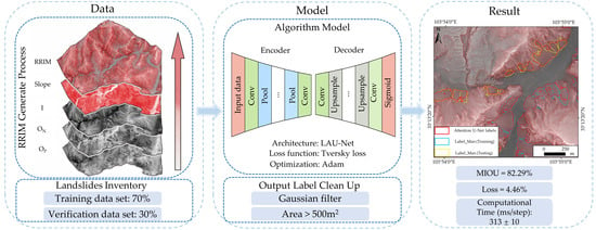
3. Detection Approach

Deep learning is a technique which is gaining momentum within the geoscientific community [53,54]. Different from other artificial intelligence, deep learning interprets images in a similar manner as a human would do. The available information is exploited to build a binary classifier based on a gridded structure where terrain and spectral data are projected to. In addition to this, though, a deep learning routine allows to solve for complex problems by including the neighboring information to any specific grid under examination [55,56]. Several deep learning routines are currently available and under continuous development. In this paper, we opted for the FCN, which is currently one of the most widely used deep learning models in image processing.

In this study, we designed a Fully Convolutional Network (FCN) to analyze LiDAR derived information and ultimately identified historical landslides. The overall approach can be summarized into three steps: (1) DEM extraction from LiDAR data; (2) manual labeling of historical landslides on LiDAR topography; (3) deep learning-based classification. The detailed flow chart of this method is shown in Figure 5.

3.1. U-Net

Image recognition can be divided into three stages: image classification, target detection, and target segmentation. Image classification determines whether a given object is contained in an image. Target detection is then used to locate the position of the target and object segmentation separates the object boundary, which is the ultimate goal of the image recognition process. Among the target segmentation tools, U-Net series is undoubtedly the most popular for FCN [57]. It consists of an end-to-end image segmentation method, which further allows the network to make pixel-level prediction and directly obtain the label map. This method is widely applied to medical image segmentation tasks [58], and has the advantages of a relatively simple architecture, fast training speed, over-fitting reduction protocols, and it is ultimately suitable even for small data sets. Similar to the medical data set, the historical landslides data set also has some problems, such as difficult data acquisition, small data samples, and various shape and size changes. Therefore, in this work we use a U-Net architecture to achieve this task, specifically for classifying, detecting, and segmenting the landslide polygons described in Section 3.2.

3.2. Attention Gate

Attention Gate is an approach proposed by Ozan Oktay in 2018 [59]. As the deep learning process deepens into the data, two levels of information are extracted. The shallower level has a better insight of the broader spatial characteristics of an image associated with lower feature information (or the landslide specifics). As for the deeper level, the opposite situation arises. The deeper the level, the more the learning process on the object of interest. Therefore, deep levels carry richer feature-specific information but lower spatial one. The additive attention coefficient formula [59] used in this paper is as follows:

$${\mathrm{q}}_{\mathrm{att}}^{\mathrm{l}}{=\mathsf{\phi }}^{\mathrm{T}}\left({\mathsf{\sigma }}_1\left({\mathrm{W}}_{\mathrm{X}}^{\mathrm{T}}{\mathrm{x}}_{\mathrm{i}}^{\mathrm{l}}{+\mathrm{W}}_{\mathrm{G}}^{\mathrm{T}}{\mathrm{g}}_{\mathrm{i}}{+\mathrm{b}}_{\mathrm{g}}\right)\right){+\mathrm{b}}_{\mathsf{\phi }}$$

(2)

$${\mathsf{\alpha }}_{\mathrm{i}}^{\mathrm{l}}{=\mathsf{\sigma }}_2\left({\mathrm{q}}_{\mathrm{att}}^{\mathrm{l}}\left({\mathrm{x}}_{\mathrm{i}}^{\mathrm{l}}{,\mathrm{g}}_{\mathrm{i}}{;\mathsf{\theta }}_{\mathrm{att}}\right)\right)$$

(3)

where ${\mathrm{q}}_{\mathrm{att}}^{\mathrm{l}}\mathrm{and} {\mathsf{\alpha }}_{\mathrm{i}}^{\mathrm{l}}$ are both of attention coefficients, ${\mathsf{\sigma }}_1$ is Relu function, ${\mathsf{\sigma }}_2$ is Sigmoid function, ${\mathrm{b}}_{\mathrm{g}} \mathrm{and} {\mathrm{b}}_{\mathsf{\phi }}$ are both of the convolution bias terms, ${\mathrm{x}}_{\mathrm{i}}$ is a pixel vector, ${\mathrm{g}}_{\mathrm{i}}$ is a gating vector, and ${\mathrm{W}}_{\mathrm{X}}^{\mathrm{T}}$, ${\mathrm{W}}_{\mathrm{G}}^{\mathrm{T}}$, and ${\mathsf{\phi }}^{\mathrm{T}}$ are all part of the convolution kernel. The role of an Attention Gate is to balance these two levels of information and combine the highly detailed information on the landslide characteristics in such a way that can be suitably generalized. This is achieved by iterating a process where the learning mechanism is based on de-emphasizing the background information while emphasizing the foreground information in a given image. The concept of emphasis or attention translates into assigning weights to specific areas of an image (where we mapped landslides) and reducing the activation value of the background to optimize the segmentation. This is the reason why this approach has gained more and more attention within the geoscientific community. In fact, landslide inventories are extremely sparse by nature. In other words, areas covered by landslides are much smaller in number and extent compared to areas where landslides have not manifested yet [60].

3.3. Lightweight Attention U-Net

We design a Lightweight Attention U-Net (LAU-Net) for historical landslides identification based on a combined U-Net and Attention Gate architecture. The network structure of LAU-Net is shown in Figure 6. This FCN model is mainly composed by encoder, bottleneck, decoder, and skip connection. During the encoding phase, input images are initially converted into an internal coding, then they are projected to 32 dimensions through the convolution and pooling layers. After this multi-stage decoding, the spatial information carried by a given image is progressively decomposed and compressed into a smaller dimensional object, whose minimum size is commonly referred to as bottleneck. After the essential information has been brought to the bottleneck, similar to the traditional U-Net, we designed a symmetrical decoder, meant to bring back the image dimensionality to its original state. The two processes describe above are then ultimately combined through a skip connection step, where the multi-scale structure of the information is brought back into the network. Below we will describe each block for clarity.

Encoder: Firstly, the binary channel images with a size of 512 × 512 pixels are transformed into a special code through the input layer, and their feature dimension and resolution remain unchanged [61]. Convolution layer (Conv) contains several feature planes, and neurons in the same feature plane share weights. We set the convolution kernel to be 3 × 3, used Relu as the activation function, and added Batch Normalization (BN) to the convolution layer. Every two convolution layers are followed by a 2 × 2 maximum subsampling (max pooling) for image down sampling. This design can reduce the connections between different layers of the network, simplify the complexity of the model, and reduce the risk of overfitting.

Bottleneck: In the bottleneck, two successive convolution layers are used to learn high dimensional features, and the characteristic dimension (256) and resolution (64 × 64) of the data remain unchanged.

Decoder: As a symmetric decoder corresponding to the encoder based on the convolution module, we also used a convolution layer with a scale of 3 × 3 for deconvolution, and every two convolution layers are followed by a 2 × 2 Upsampling layer. Each Upsampling layer reduces the feature dimension of data to half of the original and improves the resolution of the feature map at the same time. After several decoding stages, the last 1 × 1 convolution layer converts the feature vectors of 32 channels into the required classification results.

Skip connection: Unlike U-Net uses copy connections to simply connect shallow features with deep ones. Attention U-Net integrates the multi-scale features extracted from the encoder and the upsampling feature through the Attention Gate, then inputs this information into decoder. Attention Gate can adjust the feature importance of landslide area, optimize the segmentation effect of landslide, and accelerate the decoding efficiency of the model.

3.4. Optimization

Even after the implementation of the LAU-Net network described above, the model could still suffer from issues related to the number and extent of landslides in an image. Specifically, this type of deep learning classifiers is usually implemented in a context where the objects of interest occupy a significant portion of a given image. For instance, in the first paper published by Oktay et al. 2018, a large portion of the body scan hosted the pancreas, or the target to be mapped. However, in the context of landslide automated mapping, the proportion of a given image occupied by landslides is usually a mere fraction of the total. In other words, the background information is several orders of magnitude larger than the foreground one would like to identify. As a result, the overall classification may still produce undesired True Positive Rates (the proportion of correctly identified landslides over the total number of landslides). To address this issue, we adopted the optimization step introduced by [62], where a generalized loss function named Tversky loss is computed as the LAU-Net evolves through the epochs. The Tversky loss function is expressed as follows:

$$\mathrm{T}\left(\mathsf{\alpha },\mathsf{\beta }\right)=\frac{{{\displaystyle \sum }}_{\mathrm{i}=1}^{\mathrm{N}}{\mathrm{p}}_{0\mathrm{i}}{\mathrm{g}}_{0\mathrm{i}}}{{{\displaystyle \sum }}_{\mathrm{i}=1}^{\mathrm{N}}{\mathrm{p}}_{0\mathrm{i}}{\mathrm{g}}_{0\mathrm{i}}+\mathsf{\alpha }{{\displaystyle \sum }}_{\mathrm{i}=1}^{\mathrm{N}}{\mathrm{p}}_{0\mathrm{i}}{\mathrm{g}}_{1\mathrm{i}}+\mathsf{\beta }{{\displaystyle \sum }}_{\mathrm{i}=1}^{\mathrm{N}}{\mathrm{p}}_{1\mathrm{i}}{\mathrm{g}}_{0\mathrm{i}}}$$

(4)

where ${\mathrm{p}}_{0\mathrm{i}}$ is the probability of pixel $\mathrm{i}$ being a landslide, and ${\mathrm{p}}_{1\mathrm{i}}$ is the probability of pixel $\mathrm{i}$ being a non-landslide. Additionally, ${\mathrm{g}}_{0\mathrm{i}}$ is 1 for a landslide pixel and 0 for a non-landslide pixel, and vice versa for the ${\mathrm{g}}_{1\mathrm{i}}$. Finally, the minimization of the loss function described above is performed by using the Adam optimization proposed by [63].

3.5. Experiment

The source code for all of the algorithms mentioned above has been implemented using the open library TensorFlow. TensorFlow offers a wide range of deep learning routines. Therefore, to test our LAU-Net architecture, we benchmarked its landslide identification performance with respect to other famous image segmentation methods. These correspond to ResU-Net, R₂U-Net, DeepLabv3, SwinU-Net, and U-Net++ [64,65,66,67,68], and these models adopt the same parameter index design as LAU-Net. All these binary classifiers, including our LAU-Net, have been run on a machine with the following characteristics:

-

3.7 GHz intel Xeon W2255 with 64 GB of RAM;

-

graphic processing unit (GPU), NVIDIA GeForce GTX 3090 card with 24 GB of RAM and reproducibility under NVIDIA Toolkit 11.0.2.

For repeatability and reproducibility, we also list the hyperparameter we opted for: (1) the learning rate is 1 × 10⁻⁵, if the model falls into the local optimal solution, it will decay by a factor of 0.7; (2) the batch size is 16; (3) the maximum number of epochs is 150.

4. Results

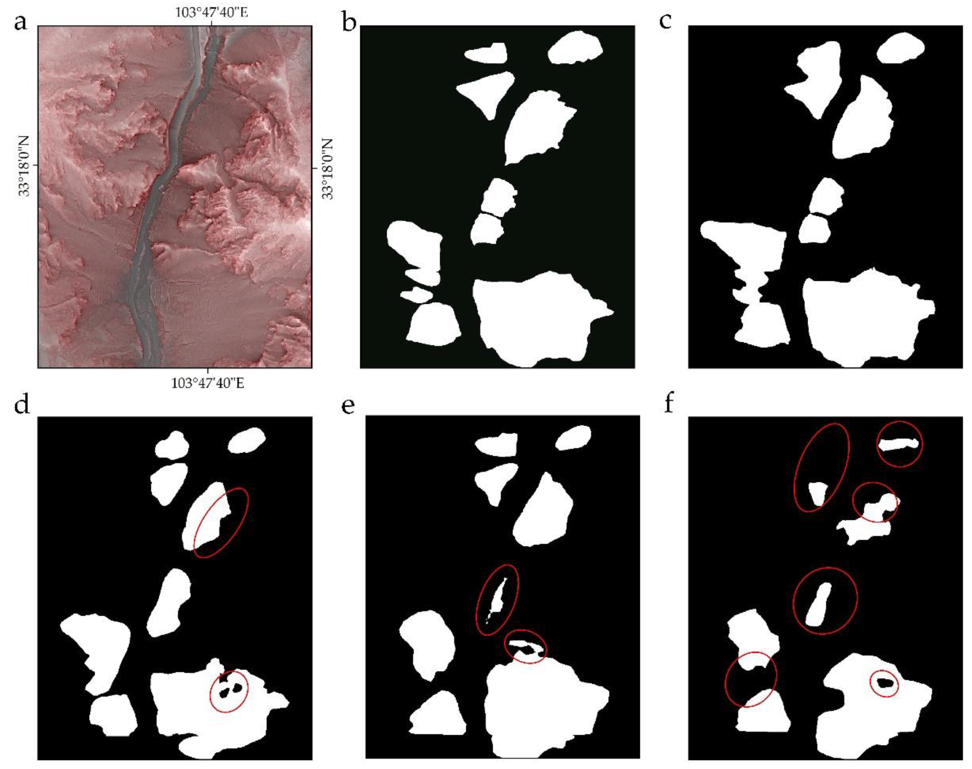
4.1. Model Validation and Comparison

All the models mentioned above are trained and compared using data sets generated by the RRIM method. In this experiment, authors apply accuracy, F1_score (%), and MIOU as the precision evaluation indexes, which is widely used as comprehensive evaluation system for image segmentation problems. According to the loss function index, we stored the testing results corresponding to the minima of each model, as well as the MIOU and the required computational time. An overview is presented in

Table 1. Results of different deep learning models.

Methods	Loss (%)	Accuracy (%)	F1 (%)	MIOU (%)	Computational Time (s/Epochs)
ResU-Net	5.53	93.86	84.11	79.15	789 ± 9
LU-Net	4.76	93.91	86.50	81.45	335 ± 15
DeepLabv3	4.61	94.27	86.67	81.57	470 ± 12
U-Net++	4.54	94.43	86.90	81.76	670 ± 10
R2U-Net	4.50	94.61	87.15	81.85	808 ± 7
SwinU-Net	4.45	95.08	87.37	82.25	1207 ± 20
LAU-Net	4.46	95.17	87.45	82.29	313 ± 10

:

As shown in Table 1, the addition of the Attention Gate channel to the Lightweight U-Net (LU-Net) network produces the lowest loss rate (loss decreased by 0.30%), and higher generalization performance in the verification set (Accuracy improved by 0.76%, MIOU improved by 0.84%, F1 improved by 0.95%). At the same time, the Attention Gate channel also improves the decoding ability of the model in the deconvolution stage. This is recorded in the computational time reports. The LAU-Net consumes less time than the LU-Net, with a time reduction of by 22 ms in each epoch. In comparison with other methods, although several other FCN models use deeper network structure and larger parameters, LAU-Net is not inferior, and it achieves the best generalization ability with a much smaller computational burden. These summary metrics support the use of LAU-Net as the most suitable FCN model for historical landslides identification, among the most common deep learning routines.

Aside from the specific metrics, in the process of model prediction, an automated procedure may still misclassify some small geomorphic units as landslides. The smallest geomorphic unit area that the method can detect is 190 m², but these smaller units are not caused by erosion factors such as landslides (e.g., Mountain flood residues, human engineering activities, etc.). The smallest landslide size in our manually mapped inventory is 544 m². Therefore, we imposed the mapping procedure to convert the landslide labels into polygons, and in the process filtered geomorphic units with an area of less than 500 m². Figure 7 shows the resulting segmentation process of our LAU-Net. The blue label marks the training data set of historical landslides, the yellow label marks the same but used for validation and the red polygons indicate the landslides boundary generated by our LAU-Net. The figure highlights a convincing segmentation effect on both the training set and the verification set, and it can accurately identify all landslides in the remote sensing images. We stress here that a LiDAR survey generates extremely finely resolved images. Thus, mosaicking them in a single image would result in a prohibitive object to be loaded in most computers. Therefore, we kept each image separate from the others. In turn, this implies that historical landslides at the edge of the original remote sensing image will inevitably be divided into several patches, in which case the landslides features should be inevitably lost. However, the model can still effectively identify them.

4.2. Identification Effect Analysis of Different Data Types

To corroborate the use of our modeling protocol, we opted to add another element of comparison. The literature reports a number of applications where landslide identification is performed by using other sources of information such as optical images, the raw DEM itself and shaded relief. Therefore, once we have proven the performance of our LAU-Net, the remaining element to be evaluated was the type of image we used. In addition to using the RRIM image (two channel), we then tested an optical image captured during a UAV survey (three channel), the raw Lidar DEM (two channel) and its hillshade derivative types (one channel). The resulting process is graphically shown in Figure 8, and numerically summarized in

Table 2. Optimal verification results for different data types.

Date Type	Loss (%)	Accuracy (%)	F1 (%)	MIOU (%)
UAV	11.28	80.56	70.28	65.2
DEM	10.37	84.41	73.37	69.56
Hillshade	8.21	87.12	79.92	76.17
RRIM	4.46	95.17	87.45	82.29

.

Out of all the data sources, the RRIM did produce the best results, being roughly 7% more accurate than the model using the shaded relief, 13% more than the DEM, and about 17% more than the model using the UAV optical information. From Figure 9, we can clearly observe that, expect for the RRIM data having good identification results, there are some problems in the identification results of other data sources. For the hillshade data, landslide ranges are not only obviously smaller, but also have the problem of cavity identification. For the DEM data, it is easy to miss small landslides during detection. Finally, for the UAV data, it loses a lot of targets and performs worst in several categories.

5. Discussion

5.1. Scale Parameter Analysis of Attention U-Net

In this paper, authors designed a LAU-Net for the specific image recognition task of historical landslides. Compared to traditional Attention U-Net (TAU-Net) with nearly 8 million parameters, this LAU-Net produces satisfactory results with one fourth of the parameters and one third of the computational burden. Figure 10 shows the training process of the LAU-Net compared to the TAU-Net, and

Table 3. Optimal verification results for LAU-Net and TAU-Net.

	LAU-Net	TAU-Net
Loss (%)	4.45	4.46
Accuracy (%)	95.20	95.17
F1 (%)	87.48	87.45
MIOU (%)	82.31	82.29
Computational Time (s/epochs)	710 ± 10	313 ± 10
Model Parameters	7.98 × 106	1.98 × 106

shows the verification result for LAU-Net and TAU-Net. As can be seen from the result, with the same optimizer and loss function, although traditional Attention U-Net performs slightly better than LAU-Net in the training set, they have markedly little differences in their generalization ability. We stress here that when solving image recognition tasks, the ability of a model to generalize its prediction is often more important than the model fitting itself. These considerations are an additional point of discussion when promoting the use of similar complex classifiers for landslide detection.

5.2. Considerations on Multiple Sources

When comparing the multiple data sources within the framework of the deep learning routine we presented, the RRIM data type achieves the best recognition effect. According to our analysis, this is due to the most detailed depiction of terrain and landform by RRIM. As shown in Figure 3, humans can clearly judge the difference between the landslide and the background through RRIM data and distinguish the source area and accumulation area of the landslide. This visual reflection can also improve the computer recognition effect. The hillshade comes relatively close to the performance provided by the RRIM counterpart. This is likely due to the capacity of the hillshade to clearly reflect geomorphic features. Thus, even historical landslides would be detectable, even more clear than when using elevation and optical alternatives. However, the shadow effect is due to peaks overlooking lowlands in the sunlight direction. The resulting darkness at these specific incidence angles may have limited the ability of our LAU-Net compared to the richer information provided by the RRIM. Interesting considerations arise in relation to the use of the DEM. In fact, this data type requires the least preprocessing to be fed to the deep learning model. However, when checking the classification results based on the DEM, many small historical landslides were misclassified. The boundary of large historical landslides appeared extremely noisy. This may be due to the limited capacity to normalize the DEM information into the deep learning process. As for the use of optical images, these produced by far the worst results. This is likely due to the dense vegetation, which inevitably masks the geomorphic signature of historical landslides. In summary, we consider RRIM data to be the most suitable data type in the context of AI-aided historical landslides identification.

5.3. Historical Landslides in Jiuzhaigou

Due to the abundant rainfall in the subtropical monsoon climate zone, and coupled with the unique mountain canyon landform, Jiuzhaigou often suffered geological disasters such as landslides and debris flows in the past. According to the records, a ravine debris flow destroyed a village which occurred at the Zaru Tample 100 years ago. Additionally, a collapse landslide occurred at Guodu in 1952 [69]. As the environment changed, the valleys and slopes where historical landslides occurred were recovered with vegetation, but it does not mean that the surface environment in the area is stable. On 7 July 2017, Jiuzhaigou earthquake induced 1988 coseismic landslides in the study area (Figure 11). It can be seen from this figure that in the regions with large scale development of historical landslides, such as regions A and B, the density of coseismic landslides induced by earthquakes is relatively high. In contrast, coseismic landslides are rarely observed in the region C, where the distribution of historical landslides is less. Therefore, the effective identification of historical landslides can not only provide support for risk assessment of geological disasters, but also deepen the spatiotemporal pattern of geological disasters before and after an earthquake in mountainous regions.

6. Conclusions

In this study, a novel approach based on LiDAR data and LAU-Net is proposed to identify historical landslides in densely vegetated mountainous areas. Authors generate RRIM through high precision data to interpret historical landslides in Jiuzhaigou. This expert-based procedure led to a total of 1949 historical landslides. A LAU-Net has then been compared to a number of competitors when it comes to AI-aided detection yet proving to produce the highest classification performance. Having confirmed this, we also compared the effects of different data types highlighting the rich information compressed into RRIM data. All these considerations indicate the use of the LAU-Net built on a RRIM foundation to be the optimal combination for historical landslides’ mapping. We believe this to be the case because the framework we proposed is capable of going deep to extract diagnostic feature information while bridging it back to the original spatial context. Despite this task being particularly complex due to the masked geomorphic signature of historical landslides—mostly by vegetation cover—the RRIM still proved to be the best candidate to reflect the body of the failed mass. We recommend a combination of appropriate data preprocessing methods and a concise network architecture to solve problems such as identifying specific geological hazards, which often yield more surprising results.

References

1. Sassa, K.; Canuti, P. Landslides-Disaster Risk Reduction; Springer Science & Business Media: Berlin/Heidelberg, Germany, 2008. [Google Scholar]
2. Huang, R.Q.; Fan, X.M. The landslide story. Nat. Geosci. 2013, 6, 325–326. [Google Scholar] [CrossRef]
3. Dai, F.C.; Lee, C.F.; Ngai, Y.Y. Landslide risk assessment and management: An overview. Eng. Geol. 2002, 64, 65–87. [Google Scholar] [CrossRef]
4. Turner, D.; Lucieer, A.; de Jong, S.M. Time Series Analysis of Landslide Dynamics Using an Unmanned Aerial Vehicle (UAV). Remote Sens 2015, 7, 1736–1757. [Google Scholar] [CrossRef]
5. Ekstrom, G.; Stark, C.P. Simple Scaling of Catastrophic Landslide Dynamics. Science 2013, 339, 1416–1419. [Google Scholar] [CrossRef] [PubMed]
6. Ardizzone, F.; Cardinali, M.; Carrara, A.; Guzzetti, F.; Reichenbach, P. Impact of mapping errors on the reliability of landslide hazard maps. Nat. Hazards Earth Syst. Sci. 2002, 2, 3–14. [Google Scholar] [CrossRef]
7. Hakan, T.; Luigi, L. Completeness Index for Earthquake-Induced Landslide Inventories. Eng. Geol. 2020, 264, 105331. [Google Scholar] [CrossRef]
8. Amatya, P.; Kirschbaum, D.; Stanley, T.; Tanyas, H. Landslide mapping using object-based image analysis and open source tools. Eng. Geol. 2021, 282, 106000. [Google Scholar] [CrossRef]
9. Zhong, C.; Liu, Y.; Gao, P.; Chen, W.; Li, H.; Hou, Y.; Nuremanguli, T.; Ma, H.J.I.J.o.R.S. Landslide mapping with remote sensing: Challenges and opportunities. Int. J. Remote Sens. 2020, 41, 1555–1581. [Google Scholar] [CrossRef]
10. Zhao, C.; Lu, Z. Remote sensing of landslides—A review. Remote Sens. 2018, 10, 279. [Google Scholar] [CrossRef]
11. Mohan, A.; Singh, A.K.; Kumar, B.; Dwivedi, R. Review on remote sensing methods for landslide detection using machine and deep learning. Trans. Emerg. Telecommun. Technol. 2021, 32, e3998. [Google Scholar] [CrossRef]
12. Solari, L.; Del Soldato, M.; Raspini, F.; Barra, A.; Bianchini, S.; Confuorto, P.; Casagli, N.; Crosetto, M. Review of Satellite Interferometry for Landslide Detection in Italy. Remote Sens 2020, 12, 1351. [Google Scholar] [CrossRef]
13. Ye, C.M.; Li, Y.; Cui, P.; Liang, L.; Pirasteh, S.; Marcato, J.; Goncalves, W.N.; Li, J. Landslide Detection of Hyperspectral Remote Sensing Data Based on Deep Learning with Constrains. IEEE J. Sel. Top. Appl. Earth Obs. Remote Sens. 2019, 12, 5047–5060. [Google Scholar] [CrossRef]
14. Catani, F.J.L. Landslide detection by deep learning of non-nadiral and crowdsourced optical images. Landslides 2021, 18, 1025–1044. [Google Scholar] [CrossRef]
15. Qin, S.; Guo, X.; Sun, J.; Qiao, S.; Zhang, L.; Yao, J.; Cheng, Q.; Zhang, Y.J.R.S. Landslide detection from open satellite imagery using distant domain transfer learning. Remote Sens 2021, 13, 3383. [Google Scholar] [CrossRef]
16. Ghorbanzadeh, O.; Shahabi, H.; Crivellari, A.; Homayouni, S.; Blaschke, T.; Ghamisi, P.J.L. Landslide detection using deep learning and object-based image analysis. Landslides 2022, 19, 929–939. [Google Scholar] [CrossRef]
17. Mondini, A.C.; Guzzetti, F.; Chang, K.T.; Monserrat, O.; Martha, T.R.; Manconi, A. Landslide failures detection and mapping using Synthetic Aperture Radar: Past, present and future. Earth-Sci. Rev. 2021, 216, 103574. [Google Scholar] [CrossRef]
18. Casagli, N.; Cigna, F.; Bianchini, S.; Hölbling, D.; Füreder, P.; Righini, G.; Del Conte, S.; Friedl, B.; Schneiderbauer, S.; Iasio, C.; et al. Landslide mapping and monitoring by using radar and optical remote sensing: Examples from the EC-FP7 project SAFER. Remote Sens. Appl. Soc. Environ. 2016, 4, 92–108. [Google Scholar] [CrossRef]
19. Haneberg, W.C.; Creighton, A.L.; Medley, E.W.; Jonas, D.A. Use of LiDAR to assess slope hazards at the Lihir gold mine, Papua New Guinea. In Proceedings of the Proceedings, International Conference on Landslide Risk Management, Vancouver, BC, Canada, 31 May–3 June 2005. [Google Scholar]
20. Glenn, N.F.; Streutker, D.R.; Chadwick, D.J.; Thackray, G.D.; Dorsch, S.J. Analysis of LiDAR-derived topographic information for characterizing and differentiating landslide morphology and activity. Geomorphology 2006, 73, 131–148. [Google Scholar] [CrossRef]
21. Schulz, W.H. Landslide susceptibility revealed by LIDAR imagery and historical records, Seattle, Washington. Eng. Geol. 2007, 89, 67–87. [Google Scholar] [CrossRef]
22. Chigira, M.; Duan, F.J.; Yagi, H.; Furuya, T. Using an airborne laser scanner for the identification of shallow landslides and susceptibility assessment in an area of ignimbrite overlain by permeable pyroclastics. Landslides 2004, 1, 203–209. [Google Scholar] [CrossRef]
23. Pawłuszek, K.; Marczak, S.; Borkowski, A.; Tarolli, P. Multi-aspect analysis of object-oriented landslide detection based on an extended set of LiDAR-derived terrain features. ISPRS Int. J. Geo-Inf. 2019, 8, 321. [Google Scholar] [CrossRef]
24. Gorsevski, P.V.; Brown, M.K.; Panter, K.; Onasch, C.M.; Simic, A.; Snyder, J. Landslide detection and susceptibility mapping using LiDAR and an artificial neural network approach: A case study in the Cuyahoga Valley National Park, Ohio. Landslides 2016, 13, 467–484. [Google Scholar] [CrossRef]
25. Jaboyedoff, M.; Oppikofer, T.; Abellan, A.; Derron, M.H.; Loye, A.; Metzger, R.; Pedrazzini, A. Use of LIDAR in landslide investigations: A review. Nat. Hazards 2012, 61, 5–28. [Google Scholar] [CrossRef]
26. Pradhan, B.; Seeni, M.I.; Nampak, H. Integration of LiDAR and QuickBird data for automatic landslide detection using object-based analysis and random forests. In Laser Scanning Applications in Landslide Assessment; Springer: Berlin/Heidelberg, Germany, 2017; pp. 69–81. [Google Scholar]
27. Eeckhaut, M.V.D.; Poesen, J.; Verstraeten, G.; Vanacker, V.; Nyssen, J.; Moeyersons, J.; van Beek, L.P.H.; Vandekerckhove, L. Use of LIDAR-derived images for mapping old landslides under forest. Earth Surf. Processes Landf. 2007, 32, 754–769. [Google Scholar] [CrossRef]
28. Gorum, T. Landslide recognition and mapping in a mixed forest environment from airborne LiDAR data. Eng. Geol. 2019, 258, 105155. [Google Scholar] [CrossRef]
29. Dou, J.; Yunus, A.P.; Merghadi, A.; Shirzadi, A.; Nguyen, H.; Hussain, Y.; Avtar, R.; Chen, Y.; Pham, B.T.; Yamagishi, H. Different sampling strategies for predicting landslide susceptibilities are deemed less consequential with deep learning. Sci Total Environ. 2020, 720, 137320. [Google Scholar] [CrossRef]
30. Wang, Y.; Fang, Z.C.; Wang, M.; Peng, L.; Hong, H.Y. Comparative study of landslide susceptibility mapping with different recurrent neural networks. Comput. Geosci. 2020, 138, 104445. [Google Scholar] [CrossRef]
31. Aditian, A.; Kubota, T.; Shinohara, Y. Comparison of GIS-based landslide susceptibility models using frequency ratio, logistic regression, and artificial neural network in a tertiary region of Ambon, Indonesia. Geomorphology 2018, 318, 101–111. [Google Scholar] [CrossRef]
32. Merghadi, A.; Yunus, A.P.; Dou, J.; Whiteley, J.; ThaiPham, B.; Bui, D.T.; Avtar, R.; Abderrahmane, B. Machine learning methods for landslide susceptibility studies: A comparative overview of algorithm performance. Earth-Sci. Rev. 2020, 207, 103225. [Google Scholar] [CrossRef]
33. Dou, J.; Yunus, A.P.; Tien Bui, D.; Merghadi, A.; Sahana, M.; Zhu, Z.; Chen, C.W.; Khosravi, K.; Yang, Y.; Pham, B.T. Assessment of advanced random forest and decision tree algorithms for modeling rainfall-induced landslide susceptibility in the Izu-Oshima Volcanic Island, Japan. Sci Total Environ. 2019, 662, 332–346. [Google Scholar] [CrossRef]
34. Amato, G.; Palombi, L.; Raimondi, V. Data–driven classification of landslide types at a national scale by using Artificial Neural Networks. Int. J. Appl. Earth Obs. Geoinf. 2021, 104, 102549. [Google Scholar] [CrossRef]
35. Meena, S.R.; Soares, L.P.; Grohmann, C.H.; van Westen, C.; Bhuyan, K.; Singh, R.P.; Floris, M.; Catani, F.J.L. Landslide detection in the Himalayas using machine learning algorithms and U-Net. Landslides 2022, 19, 1209–1229. [Google Scholar] [CrossRef]
36. Ghorbanzadeh, O.; Blaschke, T.; Gholamnia, K.; Meena, S.R.; Tiede, D.; Aryal, J. Evaluation of Different Machine Learning Methods and Deep-Learning Convolutional Neural Networks for Landslide Detection. Remote Sens 2019, 11, 196. [Google Scholar] [CrossRef]
37. Tavakkoli Piralilou, S.; Shahabi, H.; Jarihani, B.; Ghorbanzadeh, O.; Blaschke, T.; Gholamnia, K.; Meena, S.; Aryal, J. Landslide Detection Using Multi-Scale Image Segmentation and Different Machine Learning Models in the Higher Himalayas. Remote Sens 2019, 11, 2575. [Google Scholar] [CrossRef]
38. Wang, H.J.; Zhang, L.M.; Yin, K.S.; Luo, H.Y.; Li, J.H. Landslide identification using machine learning. Geosci. Front. 2021, 12, 351–364. [Google Scholar] [CrossRef]
39. Li, X.J.; Cheng, X.W.; Chen, W.T.; Chen, G.; Liu, S.W. Identification of Forested Landslides Using LiDar Data, Object-based Image Analysis, and Machine Learning Algorithms. Remote Sens 2015, 7, 9705–9726. [Google Scholar] [CrossRef]
40. Tang, X.; Liu, M.; Zhong, H.; Ju, Y.; Li, W.; Xu, Q. MILL: Channel Attention–based Deep Multiple Instance Learning for Landslide Recognition. ACM Trans. Multimed. Comput. Commun. Appl. 2021, 17, 1–11. [Google Scholar] [CrossRef]
41. Bragagnolo, L.; Rezende, L.R.; da Silva, R.V.; Grzybowski, J.M.V. Convolutional neural networks applied to semantic segmentation of landslide scars. Catena 2021, 201. [Google Scholar] [CrossRef]
42. Ju, Y.; Xu, Q.; Jin, S.; Li, W.; Dong, X.; Guo, Q. Automatic Object Detection of Loess Landslide Based on Deep Learning. Geomat. Inf. Sci. Wuhan Univ. 2020, 45, 1747–1755. [Google Scholar] [CrossRef]
43. Fang, B.; Chen, G.; Pan, L.; Kou, R.; Wang, L.J.I.G.; Letters, R.S. GAN-based siamese framework for landslide inventory mapping using bi-temporal optical remote sensing images. IEEE Geosci. Remote Sens. Lett. 2020, 18, 391–395. [Google Scholar] [CrossRef]
44. Ju, Y.; Xu, Q.; Jin, S.; Li, W.; Su, Y.; Dong, X.; Guo, Q.J.R.S. Loess Landslide Detection Using Object Detection Algorithms in Northwest China. Remote Sens 2022, 14, 1182. [Google Scholar] [CrossRef]
45. Yi, Y.N.; Zhang, Z.J.; Zhang, W.C.; Jia, H.H.; Zhang, J.Q. Landslide susceptibility mapping using multiscale sampling strategy and convolutional neural network: A case study in Jiuzhaigou region. Catena 2020, 195, 104851. [Google Scholar] [CrossRef]
46. Fan, X.; Scaringi, G.; Xu, Q.; Zhan, W.; Dai, L.; Li, Y.; Pei, X.; Yang, Q.; Huang, R. Coseismic landslides triggered by the 8th August 2017 Ms 7.0 Jiuzhaigou earthquake (Sichuan, China): Factors controlling their spatial distribution and implications for the seismogenic blind fault identification. Landslides 2018, 15, 967–983. [Google Scholar] [CrossRef]
47. Wang, F.; Fan, X.; Yunus, A.P.; Siva Subramanian, S.; Alonso-Rodriguez, A.; Dai, L.; Xu, Q.; Huang, R. Coseismic landslides triggered by the 2018 Hokkaido, Japan (Mw 6.6), earthquake: Spatial distribution, controlling factors, and possible failure mechanism. Landslides 2019, 16, 1551–1566. [Google Scholar] [CrossRef]
48. Luo, L.G.; Lombardo, L.; van Westen, C.; Pei, X.J.; Huang, R.Q. From scenario-based seismic hazard to scenario-based landslide hazard: Rewinding to the past via statistical simulations. Stoch. Environ. Res. Risk Assess. 2021, 1–22. [Google Scholar] [CrossRef]
49. Gong, P.; Liu, H.; Zhang, M.N.; Li, C.C.; Wang, J.; Huang, H.B.; Clinton, N.; Ji, L.Y.; Li, W.Y.; Bai, Y.Q.; et al. Stable classification with limited sample: Transferring a 30-m resolution sample set collected in 2015 to mapping 10-m resolution global land cover in 2017. Sci. Bull. 2019, 64, 370–373. [Google Scholar] [CrossRef]
50. Zhang, S.; Li, X.; She, J. Error assessment of grid-based terrain shading algorithms for solar radiation modeling over complex terrain. Trans. GIS 2019, 24, 230–252. [Google Scholar] [CrossRef]
51. Chiba, T.; Kaneta, S.I.; Suzuki, Y. Red relief image map: New visualization method for three dimensional data. Int. Arch. Photogramm. Remote Sens. Spat. Inf. Sci. 2008, 37, 1071–1076. [Google Scholar]
52. Kaneda, H.; Chiba, T. Stereopaired Morphometric Protection Index Red Relief Image Maps (Stereo MPI-RRIMs): Effective Visualization of High-Resolution Digital Elevation Models for Interpreting and Mapping Small Tectonic Geomorphic FeaturesStereo MPI-RRIMs: Effective Visualization of High-Resolution Digital Elevation Models. Photogramm. Eng. Remote Sens. 2019, 109, 99–109. [Google Scholar] [CrossRef]
53. Reichstein, M.; Camps-Valls, G.; Stevens, B.; Jung, M.; Denzler, J.; Carvalhais, N.; Prabhat. Deep learning and process understanding for data-driven Earth system science. Nature 2019, 566, 195–204. [Google Scholar] [CrossRef]
54. Zhang, L.P.; Zhang, L.F.; Du, B. Deep Learning for Remote Sensing Data A technical tutorial on the state of the art. IEEE Geosci. Remote Sens. Mag. 2016, 4, 22–40. [Google Scholar] [CrossRef]
55. Robson, B.A.; Bolch, T.; MacDonell, S.; Holbling, D.; Rastner, P.; Schaffer, N. Automated detection of rock glaciers using deep learning and object-based image analysis. Remote Sens. Env. 2020, 250, 112033. [Google Scholar] [CrossRef]
56. Ma, L.; Liu, Y.; Zhang, X.L.; Ye, Y.X.; Yin, G.F.; Johnson, B.A. Deep learning in remote sensing applications: A meta-analysis and review. ISPRS J. Photogramm. Remote Sens. 2019, 152, 166–177. [Google Scholar] [CrossRef]
57. Ronneberger, O.; Fischer, P.; Brox, T. U-net: Convolutional networks for biomedical image segmentation. In Proceedings of the International Conference on Medical Image Computing and Computer-Assisted Intervention, Munich, Germany, 5–9 October 2015; pp. 234–241. [Google Scholar]
58. Falk, T.; Mai, D.; Bensch, R.; Cicek, O.; Abdulkadir, A.; Marrakchi, Y.; Bohm, A.; Deubner, J.; Jackel, Z.; Seiwald, K.; et al. U-Net: Deep learning for cell counting, detection, and morphometry. Nat Methods 2019, 16, 67–70. [Google Scholar] [CrossRef]
59. Oktay, O.; Schlemper, J.; Folgoc, L.L.; Lee, M.; Heinrich, M.; Misawa, K.; Mori, K.; McDonagh, S.; Hammerla, N.Y.; Kainz, B.J.a.p.a. Attention u-net: Learning where to look for the pancreas. Comput. Sci. 2018. [Google Scholar] [CrossRef]
60. Lian, S.; Luo, Z.M.; Zhong, Z.; Lin, X.; Su, S.Z.; Li, S.Z. Attention guided U-Net for accurate iris segmentation. J. Vis. Commun. Image Represent. 2018, 56, 296–304. [Google Scholar] [CrossRef]
61. Jiang, X.; Wang, Y.; Liu, W.; Li, S.; Liu, J. CapsNet, CNN, FCN: Comparative Performance Evaluation for Image Classification. Int. J. Mach. Learn. Comput. 2019, 9, 840–848. [Google Scholar] [CrossRef]
62. Salehi, S.S.M.; Erdogmus, D.; Gholipour, A. Tversky loss function for image segmentation using 3D fully convolutional deep networks. In Proceedings of the International Workshop on Machine Learning in Medical Imaging, Quebec City, QC, Canada, 10 September 2017; pp. 379–387. [Google Scholar]
63. Kingma, D.P.; Ba, J. Adam: A method for stochastic optimization. arXiv 2014, arXiv:1412.6980. [Google Scholar] [CrossRef]
64. Qi, W.; Wei, M.; Yang, W.; Xu, C.; Ma, C. Automatic mapping of landslides by the ResU-net. Remote Sens 2020, 12, 2487. [Google Scholar] [CrossRef]
65. Alom, M.Z.; Hasan, M.; Yakopcic, C.; Taha, T.M.; Asari, V.K. Recurrent residual convolutional neural network based on u-net (r2u-net) for medical image segmentation. arXiv 2018. [Google Scholar] [CrossRef]
66. Cui, H.; Liu, X.; Huang, N. Pulmonary vessel segmentation based on orthogonal fused u-net++ of chest CT images. In Proceedings of the International Conference on Medical Image Computing and Computer-Assisted Intervention, Shenzhen, China, 13–17 October 2019; pp. 293–300. [Google Scholar]
67. Cao, H.; Wang, Y.; Chen, J.; Jiang, D.; Zhang, X.; Tian, Q.; Wang, M. Swin-unet: Unet-like pure transformer for medical image segmentation. arXiv 2021, arXiv:2105.05537. [Google Scholar]
68. Chen, L.-C.; Zhu, Y.; Papandreou, G.; Schroff, F.; Adam, H. Encoder-decoder with atrous separable convolution for semantic image segmentation. In Proceedings of the European Conference on Computer Vision (ECCV), Munich, Germany, 8–14 September 2018; pp. 801–818. [Google Scholar]
69. Daquan, Z.; Maoqi, X. An approach to mass movements in the Jiuzhaigou catchment. Nat. Hazards 1993, 8, 141–151. [Google Scholar] [CrossRef]
Figure 1. Geographical location of the study area ((a). Optical image of UAV in study area. (b). The geographical location of Jiuzhaigou County in China. (c). The location of the study area in Jiuzhaigou County).
Remotesensing 14 04357 g001
Figure 2. Framework of RRIM generation process.
Remotesensing 14 04357 g002
Figure 3. The visual comparison of historical landslides in different data ((a). UAV optical image. (b). DEM. (c). Hillshade. (d). RRIM. (e). Landslide feature with RRIM).
Remotesensing 14 04357 g003
Figure 4. Distribution of historical landslide samples.
Remotesensing 14 04357 g004
Figure 5. Schematic diagram of automatic historical landslides identification process.
Remotesensing 14 04357 g005
Figure 6. LAU-Net network architecture.
Remotesensing 14 04357 g006
Figure 7. Comparison of historical landslide profiles identified by computer intelligence and interpreted by humans (Regions (a,b) are used to magnify the prediction results of the model).
Remotesensing 14 04357 g007
Figure 8. The training process of different data in LAU-Net ((a). F1_score index of Verification set, (b). Loss function index of verification set).
Remotesensing 14 04357 g008
Figure 9. Comparison of identification effects of multi-source data and the red circles highlight where the result is abnormal ((a) RRIM. (b) The reference map of historical landslides, where black and white pixels represent no landslides and landslides. (c) Recognition results by RRIM. (d) Recognition results by hillshade. (e) Recognition results by DEM. (f) Recognition results by UAV).
Remotesensing 14 04357 g009
Figure 10. Comparison of various indicators between traditional Attention U-Net and LAU-Net ((a). Loss function index of training set. (b). Loss function index of verification set. (c). F1_score index of training set. (d). F1 function index of verification set).
Remotesensing 14 04357 g010
Figure 11. Distribution diagram of coseismic landslides and historical landslides ((A). Schematic diagram of landslides distribution in Jiuzhai paradise area. (B). Schematic diagram of landslides distribution in Panda sea area. (C) The region where observed little coseismic landslides and historical landslides).
Remotesensing 14 04357 g011