Machine Learning-Based Rockfalls Detection with 3D Point Clouds, Example in the Montserrat Massif (Spain)

Abstract

Rock slope monitoring using 3D point cloud data allows the creation of rockfall inventories, provided that an efficient methodology is available to quantify the activity. However, monitoring with high temporal and spatial resolution entails the processing of a great volume of data, which can become a problem for the processing system. The standard methodology for monitoring includes the steps of data capture, point cloud alignment, the measure of differences, clustering differences, and identification of rockfalls. In this article, we propose a new methodology adapted from existing algorithms (multiscale model to model cloud comparison and density-based spatial clustering of applications with noise algorithm) and machine learning techniques to facilitate the identification of rockfalls from compared temporary 3D point clouds, possibly the step with most user interpretation. Point clouds are processed to generate 33 new features related to the rock cliff differences, predominant differences, or orientation for classification with 11 machine learning models, combined with 2 undersampling and 13 oversampling methods. The proposed methodology is divided into two software packages: point cloud monitoring and cluster classification. The prediction model applied in two study cases in the Montserrat conglomeratic massif (Barcelona, Spain) reveal that a reduction of 98% in the initial number of clusters is sufficient to identify the totality of rockfalls in the first case study. The second case study requires a 96% reduction to identify 90% of the rockfalls, suggesting that the homogeneity of the rockfall characteristics is a key factor for the correct prediction of the machine learning models.

1. Introduction

Rockfalls are one of the most frequent and dangerous phenomena in mountainous areas [1,2]. They consist of rock fragments that are detached from a steep rock face by descending rapidly while performing a free fall, rolling or bouncing [3]. They are essentially gravitational events triggered at high speed, which may cause severe damage to buildings, infrastructures, and lifelines due to their spatial and temporal frequency and their intensity (kinetic energy) [4,5]. Rockfall risk in mountainous areas is increasing as the population and economic activity increase [6]. Therefore, rigorous hazard and risk analyses are essential to provide the best possible protection measures [5]. The rockfall magnitude–frequency relationship is an important component of hazard and risk assessment for dangerous slopes, which can be evaluated using a rockfall inventory [7,8]. In addition to the magnitude–frequency relationship, information on the location of the source zone and the shape of the block can be useful for understanding the failure processes that operate on the slope [7,9]. Thus, the identification and characterization of rockfall events on rock slopes constitute a necessary task for risk assessment and mitigation.

Nowadays, the development of remote sensing techniques such as terrestrial laser scanner (TLS) based on the lidar (light detection and ranging) technique and digital photogrammetry has been advantageous where steep and unstable slopes make conventional field data collection dangerous and impractical [10]. Such remote sensing techniques greatly facilitate the collection of a significant amount of high-quality data, i.e., 3D point clouds. As a result, the studies on the identification of changes in rock slopes and the acquisition of rockfall inventories are rapidly increasing [11,12,13].

1.1. Rockfall Source Analysis from Point Cloud Data

Recently, many applications of rockfall analysis employing 3D point cloud data produced from TLS or photogrammetry have been developed. In terms of rockfall source detection, Santana et al. [14] and Corominas et al. [15] identify rockfall scars and calculate their volumes, using a point cloud by means of identifying discontinuity surfaces and the minimum spacing between them. Other authors used single point clouds to perform rock cliff stability analysis such as Fanti et al. [16] and Mazzanti et al. [17]. However, the development of change detection algorithms, such as M3C2 [18], facilitates the identification of areas of loss on slopes (i.e., rockfalls) among subsequent 3D point clouds. The location, volume, and shape of rockfalls on the slope can be calculated and populated into a database. In this respect, Tonini and Abellan [19] detect and extract individual rockfall events that occurred during a time span by using clustering algorithms. Van Veen et al. [7] applied these methods to a hazardous slope that presents rockfall hazards to the CN Rail line in British Columbia, to build a database of rockfalls. Janeras et al. [20] quantified the frequency of small or even previously unnoticed rockfalls in Montserrat massif near Barcelona (NE Spain). Bonneau et al. [21] describe the rationale and consequences of measuring the dimensions of 3D rockfall objects obtained from successive point clouds, and introduce two unique algorithms to standardize the process. Bonneau and Hutchinson [22] use high-resolution photographs to validate changes described in TLS data analysis and to follow deposition patterns in a dynamic cliff talus system. Furthermore, in order to monitor progressive failures, change detection systems have been used to identify precursory indicators, such as cleft opening or pre-failure deformations [23,24,25].

The interval between point cloud acquisitions has a significant impact on both the identification of rockfall precursory indicators and the categorization of rockfalls with their shape and volume from change detection approaches [7,19,26]. In order to better understand progressive failures and to improve the magnitude–frequency relationship to characterize the rockfall activity on a rock cliff, fixed systems have been developed to acquire data with a high frequency or in quasi real-time [27,28,29]. Consequently, a large amount of high-quality data acquired by TLS and photogrammetry in high-frequency monitoring approaches has begun to overwhelm users [26,30]. Consequently, the process of change identification in rock cliffs from lidar or photogrammetric 3D point clouds has undergone a thorough development in the last years to address and improve the current time-consuming analytical methods.

The algorithms developed to automate the processes for the detection of change from multi-temporal 3D point cloud comparison usually follow these steps (see comparative in Figure 1): (a) point cloud classification to remove objects without interest (e.g., vegetation, or misplaced points due to moisture or edge effects); (b) point clouds alignment (i.e., placing the different point clouds in the same reference system); (c) computing differences between point clouds; (d) clustering neighboring points with significant differences, and (e) classification of clusters according to their nature (e.g., bedrock, vegetation, edge effects, soil, rockfall, or deformation) [24,25,31]. Numerous initiatives have been made to automate intelligent pipelines using machine learning techniques such as deep learning and neural networks, which have made tremendous progress, particularly in the task of identifying rockfalls. However, in this proposal we try to automate not only the identification of rockfalls but also the evolution of the overall process, as data are collected over time until the final prediction is obtained.

1.2. Improvements on Rockfall Detection from Point Cloud Comparison including Machine Learning Algorithms

Recent research studies utilize mainly machine learning algorithms for rock-slope and landslide monitoring and analysis ([32] and references therein). However, few studies address the automation of rockfall detection including machine learning processes in the different steps of the point cloud comparison.

Since differences in vegetation, soil, anthropic actions or rockfalls lead to inaccuracies in the point clouds alignment process, the first step for point clouds comparison is the filtering of unwanted areas of each point cloud, such as vegetation or edges, to infer optimal change detection and posterior rockfall classification [29]. It is sometimes difficult to separate bedrock from vegetation or another class of surface in terms of time consumption or supervision of the result. Different approaches consist of manually generating masks with the areas of interest in the point cloud scene [30,33]. Furthermore, based on the possibilities of analyzing the lidar return intensity, Williams et al. [29] remove points with certain criteria, thereby reducing uncertainty. Other approaches, such as CANUPO [34], classify regions of interest, training binary classifiers and combining them with some rules. Weidner et al. [33] present a random forest machine learning approach that improves the classification accuracy and efficiency compared to CANUPO. Other approaches, such as surface interpolation concepts with the cloth simulation filter (CSF, [35]), or multiscale curvature classification MCC [36], are also strategies for identifying relevant classes of surfaces (e.g., bedrock, soils, or vegetation). This step for removing unwanted points can be carried out, providing that the success of this operation is ensured. However, in cliffs with complex morphology and compounded of different materials (rock, soil, talus, vegetation, etc.), it is difficult to encompass a good automatic classification, requiring time-consuming manual filtering.

Other advances have focused on adapting and improving change detection algorithms. While the most commonly used algorithm is Multiscale Model-to-Model Cloud Comparison (M3C2) [18], other authors such as Williams et al. [29] and Kromer et al. [37] improved the overall accuracy of change detection and streamlined the workflow when applied to large time series scan datasets. For the purpose of recognizing rockfall events, additional developments have been offered by DiFrancesco et al. [4], indicating enhancements to the performance of the change algorithm. According to these authors, the procedure of filtering away incorrect clusters (such as vegetation, edge faults, snow, or dampness) is often either disregarded or carried out manually once individual objects are recovered from the point cloud using clustering.

Several authors have developed different approaches to gain objectivity, efficiency, or productivity in cluster classification. Supervised or manual classification is one of the most commonly employed techniques, but identifying rockfalls according to several classes is a tedious and laborious undertaking that can sometimes become subjective and dependent on the criteria used by the expert classifiers [7,38,39]. More recent proposals are based on statistical model classifications and machine learning studies such as those by Schovanec et al. [30]. The aforementioned study proposes a way of filtering clusters using the random forest algorithm. However, they do not address the data imbalance issues (lower number of rockfall labeled clusters vs. higher number of no-rockfall clusters), caused by the sensitivity of the sensor and the complexity of the analyzed scene [32]. In this context, Zoumpekas et al. [32] focus their work on identifying 3D point cloud clusters of the rockfall class while dealing with an imbalanced classification task.

In this paper we propose a cluster classification method based on the developments by Zoumpekas et al. [32], using different machine learning models and resampling strategies in the classification of rockfall clusters in order to implement prediction models. In our opinion, machine learning algorithms are better trained by using cluster features than using 3D point characteristics. Consequently, we propose some adaptations of the already accepted algorithms for change detection (M3C2 by Lague et al. [18]) and clustering (Density-Based Spatial Clustering of Applications with Noise, DBSCAN by Ester et al. [40]) to compute geometric features. Thus, a total of 33 features are used to characterize clusters to improve the training stage for the machine learning classification. In this study, certain characteristics of the clusters are proposed to be able to feed the learning models. Although there could be more or others, in our proposal a global framework based on machine learning is presented, but the study and validation of the elicitation of the characteristics (features) used by the learning models is outside the scope of this proposal.

Zoumpekas et al. [32] concentrate on the machine learning training stage, analyzing the associated problems and proposing a series of solutions and tools (data normalization, balancing techniques, cross-validation, hyper-parameterization, classifier models, tools to identify the best classifier model). Our current proposal shows the adaptation of existing algorithms to better characterize clusters and incorporating the approaches proposed by Zoumpekas et al. [32] to solve the problems encountered in the training stage. The proposed intelligent framework is performed in two different rock cliffs of the Montserrat massif (NE Spain) to test the response of prediction models against rockfalls of different characteristics, in terms of volume and shape. This framework provides a novel ready-to-use point cloud machine learning software targeted at rockfall identification, which may be incorporated as a stand-alone component in a rockfall hazard decision support system. The main contributions of this work are the following:

• We propose an extension of the full end-to-end intelligent framework proposed by Zoumpekas et al. [32] for rockfall detection handling highly imbalanced data by reducing the number of clusters in our data. We further introduce geological properties to the framework itself.
• We implement the proposed intelligent system with real data from two different cliffs of Montserrat massif (NE Spain) to validate its efficacy and effectiveness.
• Our results show great performance and robustness, which is of paramount importance in rockfall detection.
• We provide a baseline methodology and a detection accuracy benchmark for future related experimental analyses.
• We have made fully accessible the applications developed in this work, the 3D point cloud data used, and an example of application in public repositories (see Section 2).

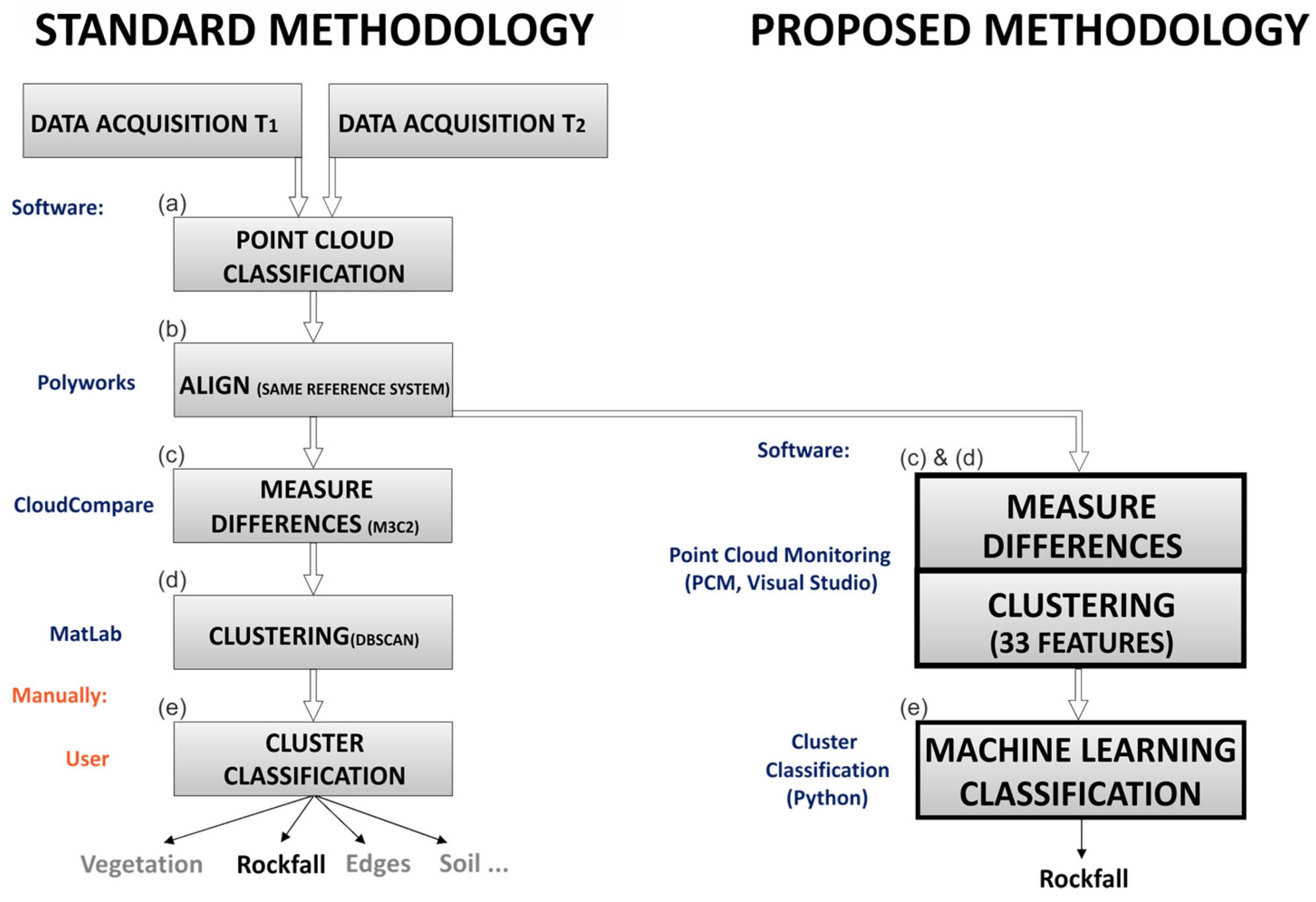
The paper is organized as follows. Section 2 exposes how these methods have been adapted to the proposed methodology, based on measuring new features that upgrade machine learning classifications. Section 3 shows the results of the study case of the Degotalls in the Montserrat massif (Barcelona, Spain), a rock cliff where the fracture pattern favors the rockfalls next to infrastructures [20].

2. Methods

In the first steps, the proposed methodology follows the standard processes of data capture, alignment, and a light manual point classification, which can be applied with the most commonly used processing software (e.g., CloudCompare [41] or Polyworks [42]). After that, the methodology is split into two steps. Firstly, the measurement of differences to create clusters with associated features, and secondly the classification of clusters to identify rockfalls (right side of Figure 1). Our contribution consists in implementing the new features necessary for characterizing clusters and classifying rockfall clusters with machine learning in order to increase the automation of the process. Thus, our methodology proposes the following four-fold contributions:

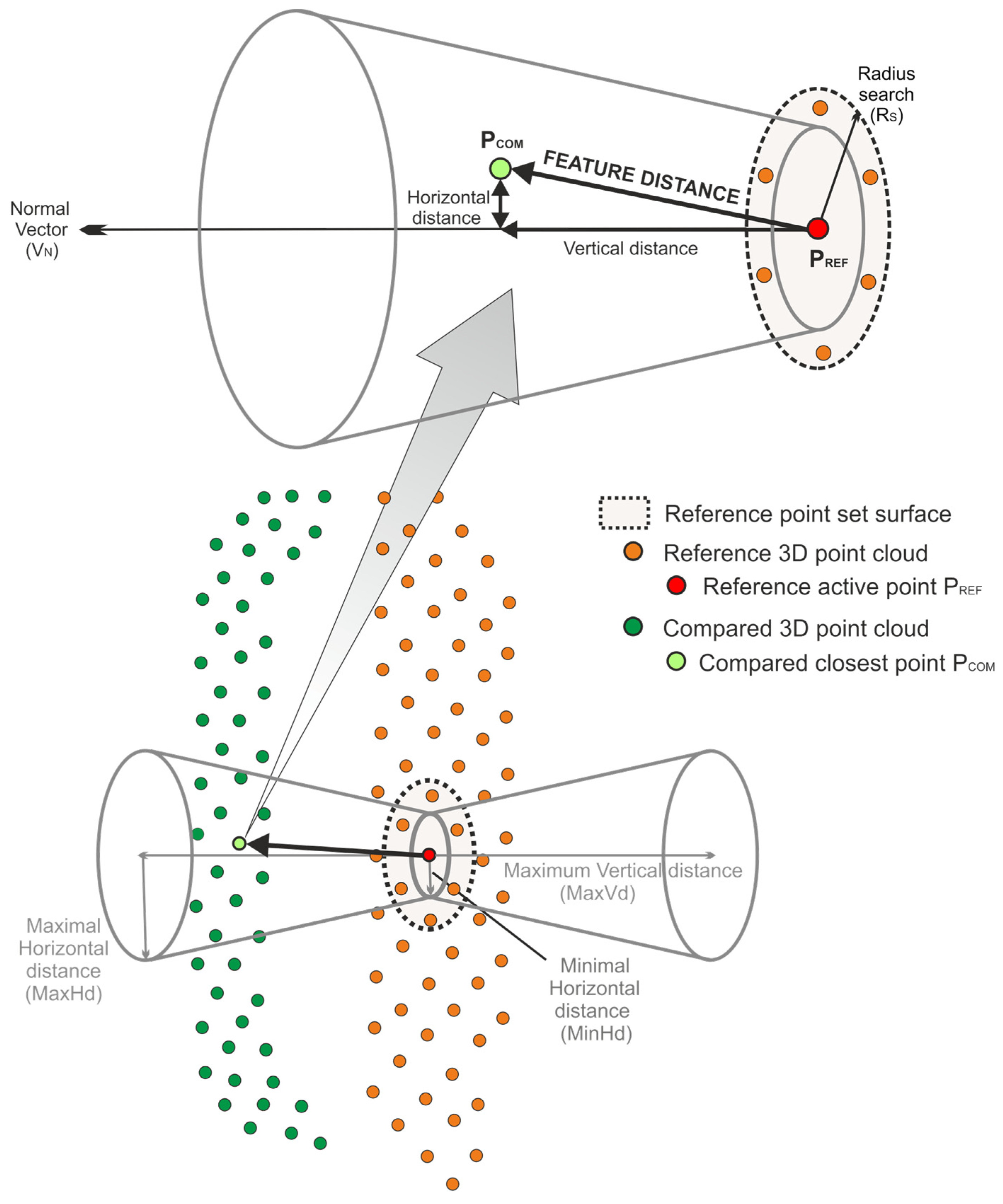
• The adaptation of the M3C2 algorithm to measure differences point-to-point and to obtain the new associated features required for the machine learning processes. The main features are geometric such as difference between point clouds, reference and compared surface orientation, indexes of coplanarity and collinearity.
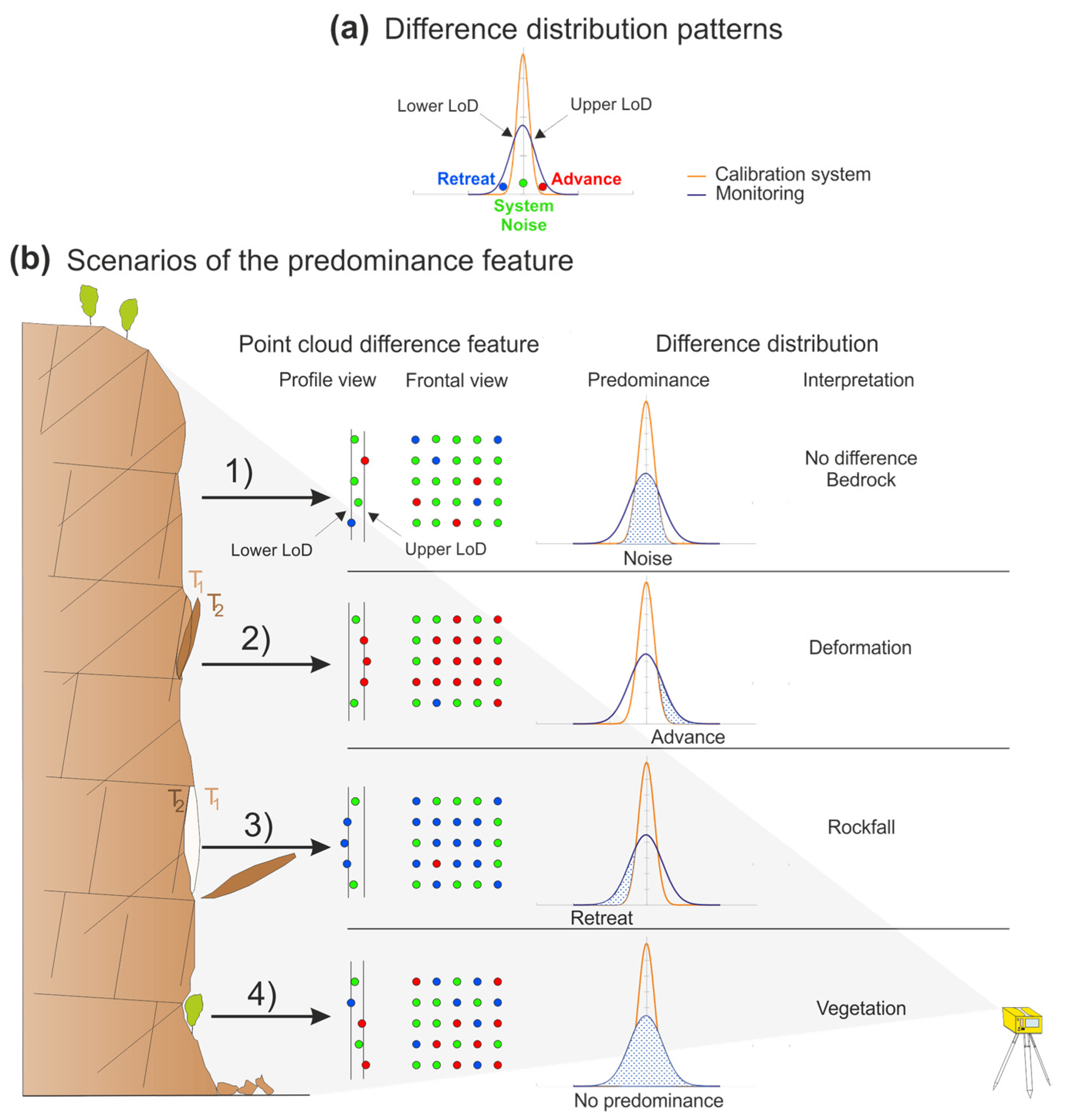
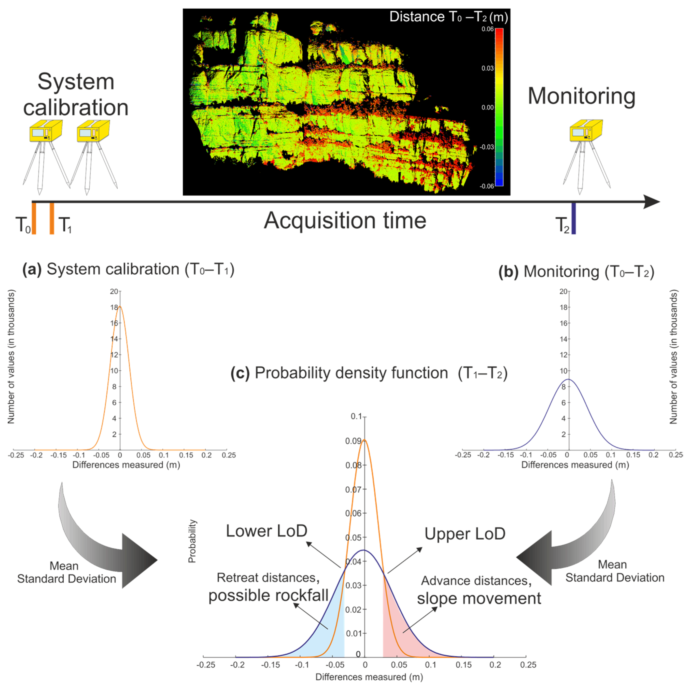
• The development of a self-calibration method to automatically define the limit of detection (LoD) and differentiate real changes in the rock cliff from the system noise.
• The adaptation of the DBSCAN algorithm for clustering point clouds and create new cluster features of predominance associated with the point differences (retreat or advance) in the cliff surface.
• The analysis of different machine learning models to classify clusters of rockfalls.

The first three methods, measurements of differences, LoD and clustering, implemented in the “Point Cloud Monitoring” software (PCM), have been developed using Visual Studio 2019 [43] and the BASIC programming language. The fourth method related to the cluster classification is called “Cluster Classification” and it has been implemented using Python programming language. All the developed applications in this research are available at the GitHub repository of the group (https://github.com/Geomodels-UB/Risknat_Detection) (accessed on 12 June 2022). The 3D point clouds, and one example can be found in the UB repository: Point Cloud: https://dataverse.csuc.cat/dataset.xhtml?persistentId=doi:10.34810/data201 (accessed on 20 July 2022). Example: https://dataverse.csuc.cat/dataset.xhtml?persistentId=doi:10.34810/data199 (accessed on 20 July 2022).

The initial data format of the methodology is a 3D point cloud format (see Appendix A for detailed information), to which the computed new features are added (see the complete list in Appendix B). The cluster format (detailed in Appendix C) is a 3D point (the center of mass of used points) which is characterized with statistical and cluster features.

2.1. Adaptation of the M3C2 Algorithm

Different strategies have been developed to measure changes in rock slope surfaces over time. The most commonly employed techniques are: (a) point-to-point [41,44]; (b) point-to-model [19,45,46]; or (c) model-to-model [4,18,25]. The M3C2 method proposed by Lague et al. [18] and implemented in the software CloudCompare [47] is one of the most commonly employed in rockfall change detection [7,22,23,30]. In this case, the difference is measured along the normal vector calculated with a set of points from the reference point cloud and projected until intersection with a set of points of the compared 3D point cloud. In accordance with the objectives, the arrangement is configured with two parameters that define a cylinder, the diameter of search around an initial point and the maximum depth [48]. The result of the point cloud comparison is a new point cloud including the feature difference (ε) as well as to the 3D coordinates and intensity or RGB.

In this work we propose an adaptation of the M3C2 method to obtain more attributes (features) that characterize rockfall clusters, which will feed the training of machine learning classifiers.

Essentially, the adaptation consists in compute features associated with the geometric relationship between reference point (initial 3D point cloud) and compared point (monitoring or second 3D point cloud). For this reason, the [49] algorithm M3C2 has been converted from model-to-model to point-to-point by changing the detection method to use real data points. Consequently, a normal (V_N in Figure 2) for each reference 3D point (see P_REF in Figure 2) is computed by means of the principal component analysis method [49] and the eigenvalues and eigenvectors method [50] with the set points selected by a radius search condition defined by the users (R_S in Figure 2). The compared point (see P_COM in Figure 2) is sought along this normal vector direction (V_N) with the closest point criterium. Thus, the feature difference is calculated with the closest point in an orthogonal direction to the reference 3D point. Likewise, the cylinder used by Lague et al. [18] is replaced by a double truncated cone or conical frustum. The user defines the maximal and the minimal horizontal distance and the maximal vertical distance (normal direction) of the search (see MaxHd, MinHd, MaxVd in Figure 2). This geometric figure allows a better fit when working with high densities of point clouds. The high densities of points reduce the distance between them, allowing to work point-to-point without the need for interpolation, especially in irregular scenarios. Monitoring always under the same conditions (TLS or camera position, point cloud density) it is strongly recommended. The process computes the normal vector as a feature at each point in both point clouds (reference and compared), decomposing the azimuth and slope values, with the aim of characterizing the surface of the rock cliff. Furthermore, the coplanarity and collinearity values are calculated as a result of applying the eigenvalues at each point of the point clouds [51].

The algorithm computes a total of 33 features (using Intensity texture, see the complete list in Appendix B, summarized in

Table 1. Summary of the new features computed with the adaptation of the M3C2 [18] algorithm implemented in PCM software. Comparison between the distances of the 3D point clouds is performed in the direction defined by the reference normal vectors. Results are associated with a new point cloud with these features.

Features	Significance
Distance	Distance between points (reference and compared)
Vertical Distance	Distance along the normal vector
Horizontal distance	Perpendicular distance to the normal vector
Angle between normal	Angularity between normal reference and compared
Direction	Direction of the normal vector with respect to the surface
Vector	Normal vector (i, j, k) for each point
Azimuth	Normal vector decomposed in orientation to North
Slope	Normal vector decomposed in orientation to horizontal
Collinearity	Distribution degree of neighboring points along a line
Coplanarity	Distribution degree of neighboring points along a plane

). All the new features are related to the geometric components of the distance (vertical and horizontal components), the angle between the two normal vectors (e.g., reference point cloud, and compared point cloud), and their direction (towards the TLS or from the TLS), and its geometric attributes are: collinearity and coplanarity.

2.2. Automatic Calibration

The LoD is the value at which the distance is considered representative of a real change or is assumed to be system noise. Thus, according to the LoD, points can be classified into three possible classes: (a) surface advance (i.e., precursory deformation); (b) surface retreat (i.e., rockfall); or (c) undetermined difference depending on the precision of the system (e.g., TLS precision, TLS–surface range, and software used). The undetermined type is not assigned to a true variation of the surfaces when the values of the difference are within the LoD limits. The value of the LoD is established by the knowledge of the user in the area or by experimental case studies [27,48]. Thus, it is necessary to quantify the LoD to distinguish between differences caused by the noise of the detection system and these corresponding to real changes in the slope. For this purpose, we propose to acquire two datasets with a time interval that is as short as possible, assuming that in this interval nothing has changed on the bedrock surface. The calculation of the differences between both point clouds (T₀–T₁) are fitted to a Gaussian distribution model in which the function depends on the mean and the standard deviation establishing the precision of the system (Figure 3a). Subsequently, when two monitoring point clouds (T₁–T₂) are compared in order to determine the real changes, the values of the differences are also fitted to another Gaussian distribution (Figure 3b). On comparison of both probability density functions, the points of intersection indicate the limit value (LoD) to be considered as system error, and therefore indicate the probability of being assigned to a real change in the cliff (Figure 3c). In fact, the values of the feature difference between the upper LoD and the lower LoD are regarded as system noise. However, values greater than the upper LoD are regarded as probable advances in the bedrock, while difference values less than the lower LoD are regarded as probable mass losses due to possible rockfalls.

Factors that define the noise of the system are varied [25] and differ in each scan. During the scan, the angle of incidence of the emitted laser pulse and its return vary according to the decrease in the perpendicularity of the scene. Distance and incidence angle affect the precision of the difference values between point clouds. We avoid this loss of precision during the calibration by using only the points belonging to surfaces perpendicular to the TLS and at a representative mean distance from the outcrop. The calibration system values (defined by mean and standard deviation) have been introduced in PCM software to calculate the upper and lower LoD during monitoring.

2.3. DBSCAN Adaptation

After computing differences, it is necessary to cluster points in accordance with this feature in order to identify and reconstruct the rockfall shapes and volumesDBSCAN algorithm [40] is widely used to cluster points [30,39,52,53,54]. The algorithm of clustering points conforms to the parameters of distance with respect to the other points, the values of the difference between point clouds, and a minimal number of points to define a cluster (parameters: eps, ε, and minPts). It is implemented in free software available in open-source libraries such as Open3d [55], Scikit-learn [56], or commercial software such as MATLAB.

This work proposes an adaptation of the DBSCAN algorithm that consists of analyzing the feature differences in the neighboring points during clustering in order to create four new features (

Table 2. New features computed with the adaptation of the algorithm DBSCAN. The results are incorporated into the cluster event as cluster feature.

Feature	Significance
Predominance	Majority class (advance, retreat, or noise)
Noise percentage	Percentage of points classified as noise according the LoD
Advance percentage	Percentage of points classified as advance according the LoD
Retreat percentage	Percentage of points classified as retreat according the LoD

); predominance, noise percentage, advance percentage, and retreat percentage. The feature predominance is defined for each reference point by the majority value classified as advance, retreat, or noise of its neighboring points according to the LoD (Figure 4). The remaining features quantify the percentage of each class in the neighboring points (advance, retreat, and noise).

Some of the features that characterize each cluster (detailed in Appendix C) have their origin in the features that characterize its points. The centroid of each cluster is represented by the center of mass of the point coordinates, computed with the principal component analysis method, and the quantifiable features are processed statistically (means and standard deviations). The specific features of each cluster, such as the volume, area or the number of points, are computed individually. The reference point clouds and the compared point clouds are triangulated separately with respect to a common plane base. The total volume corresponds to the sum of these volumes, and always preserves the positive and negative direction with respect to the TLS position.

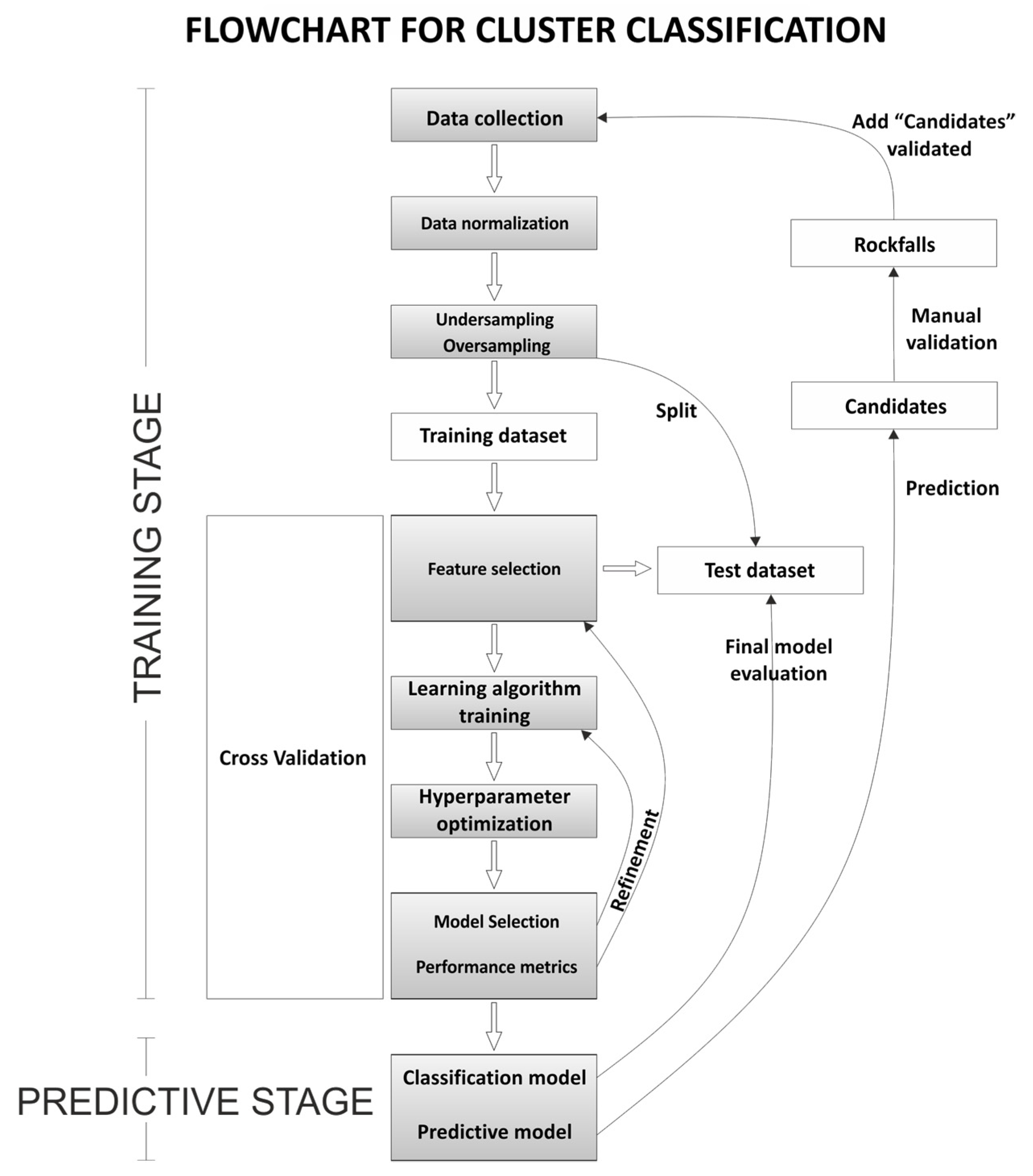
2.4. Cluster Classification

On completion of the PCM software stage for the creation of clusters, the cluster classification step categorize clusters as rockfalls and not. This step involves different stages (see flowchart in Figure 5): (1) the training stage to train the models using a hand labeled dataset of clusters of rockfalls, and (2) the predictive (or testing) stage to identify non-classified clusters. As input of the system, we manually labeled clusters as “Candidate”, if they contain rockfalls validated with high-resolution images, and 0 otherwise (i.e., “Unknown”). We propose the categorization of “Candidate” to determine cluster that contain possible candidates to be a rockfall, and “Unknown” for clusters attributable to the rest of events. After that, we proceed with the data normalization to convert all the features in the range [0–1]. This process is necessary to avoid the classification models weigh more on some features than others.

In fact, this prior manual classification must guarantee a minimum number of clusters labeled as rockfalls. However, some scenarios in the training stage may present an imbalance between the number of clusters in each class due to the large number of “Unknown” clusters, such as in the case study of the Montserrat massif [20,57]. The number of items resulting from clustering differences, mostly consisting of the “Unknown” class (attributable to vegetation or edge effects), may range from tens to about one hundred times higher with respect to the validated “Candidate”. To correct this imbalance, Zoumpekas et al. [32] propose the implementation of resample strategies, either by reducing the majority classes (undersampling method) or synthetically increasing the number of minority classes (oversampling method). The resample methods implemented in the proposed methodology are shown in

Table 3. Different resampling methods to correct the imbalance between classes.

Undersampling	Oversampling
Cluster Centroids	SMOTE [58] (Synthetic Minority Oversampling Technique)
Cluster Representatives [59]	ADASYN [60] (Adaptive Synthetic Sampling)
	SPIDER [61] (Selective Pre-processing of Imbalanced Data) SWIM [62] (Sampling with the Majority) Polynom-fit-SMOTE [63]
	ProWsyn [64] (Proximity Weighted Synthetic) SMOTE-IPF [65] (SMOTE-Iterative Partitioning Filter) LEE [66]
	SMOBD [67] (Synthetic Minority Over-sampling Based on Samples Density) G-SMOTE [68] (Geometric-SMOTE) LVQ-SMOTE [69] (Learning Vector Quantization-SMOTE) Assembled-SMOTE [70]
	SMOTE-TomekLinks [71]

.

The classification models used in this refinement process corresponds to two families, depending on the number of algorithms used in each model. The simplest “Single base learning”, i.e., models that just use one strategy to learn through a dataset and those that use multiple strategies, commonly named as “Ensemble learning” [72].

Table 4. Different classifier models used to learn and define a pipeline with the nomenclature proposed by Ma et al. [72].

Single Base	Ensemble
Linear Discriminant Analysis [73]	AdaBoost Classifier [74]
Quadratic Discriminant Analysis [73]	Random Forest Classifier [73]
K-Nearest Neighbors Classifier [73]	Extra Trees Classifier [75]
Gaussian Naive Bayes [73]	XGBoost Classifier [76]
Decision Tree Classifier [73]
Support Vector Classifier [77]
Multi-Layer Perceptron Classifier [78]

shows the methods contemplated in this study.

It should be noted that we use a stratified 10-fold cross-validation technique to assess the effectiveness of the parameters that define each classification model, evaluating and checking the models for independent datasets in a resampling procedure. The design of each model architecture is inferred by hyper-parameter tuning optimizing the scoring recall. Note that with the 10-fold cross-validation, we perform training on the 9 subsets, but we leave one subset for the evaluation of the trained model. Thus, we iterate 10 times with a different subset reserved for testing purpose each time.

In order to find out the classification model and its configuration (i.e., the hyper-parameters in

Table 5. The table shown the configuration for the exhaustive search of the best parameter in each classifier model. The best parameter is implemented to obtain the best «scoring recall».

Classifier Models	Hyper-Parameters
Linear Discriminant Analysis	Solver: svd, lsqr, eigen
Quadratic Discriminant Analysis	Reg param: 0.1, 0.3, 0.5
K-Nearest Neighbors Classifier	Number of neighbors: 1, 17
Gaussian Naive Bayes	Var smoothing: logspace (0, −9, num = 100)
Decision Tree Classifier	Criterion: gini, entropy; Maximum depth: 3–15
Support Vector Classifier	C: 0.1, 1, 10; Gamma: 1, 0.01; Kernel: rbf
Multi-Layer Perceptron Classifier AdaBoost Classifier	Solver: lbfgs, SGD, ADAM; Activation: relu; Hidden layer sizes: 50, 100, 150 Number of estimators: 1–50; Learning rate: 0.2
Random Forest Classifier	Number of estimators: 1–20;
Extra Trees Classifier	Criterion: gini, entropy; Maximum depth: 3–15 Number of estimators: 1–20;
XGBoost Classifier	Criterion: gini, entropy; Maximum depth: 3–15 Nthread: 4; Booster: gblinear, gbtree; Missing: −999 Learning rate: 0.1, 0.2, 0.3; Number of estimators: 50, 100, 500; Seed: 1337; Disable default metric: True

and the feature selection) that obtain the best “scoring recall”, we performed a set of experiments involving the analysis of different classification models summarized in Table 4. We symbolize this analysis as a “Refinement” in Figure 5.

Once the classifier models are trained with the optimal score for recall results (fraction of rockfalls that are successfully identified), the predictor models are executed with a new monitoring collection dataset that contains unlabeled clusters. The results of the prediction models provide a list of clusters labeled as “Candidate”. The accuracy of the prediction models poses two challenges: (a) to achieve a low number of false positives (FP), i.e., clusters classified as “Candidate” but which do not correspond to real rockfalls; and (b) to avoid false negatives (FN), i.e., clusters of real rockfalls but classified as “Unknown”. The first challenge requires a great effort from the geologist to validate false cluster, while the second makes it impossible to validate candidate clusters of rockfalls. Therefore, these goals of making the real number of rockfalls is equal to TP are achieved, and the values of FP and FN are as close to zero or becomes zero. Thus, unlike with a classical methodology for selecting the best model using accuracies [32], we evaluate the results of the prediction by analyzing manually high-resolution images of the landscape, searching true positive, false positive, and false negative values.

This manual validation of the automatically classified clusters in relation to the observation of high-resolution images of the outcrop, allows to guarantee the validity of the labelling for future training and predictions. The clusters validated with this procedure as “Candidate” are added to the “Labeled Clusters” dataset to feed new trainings in future scenarios.

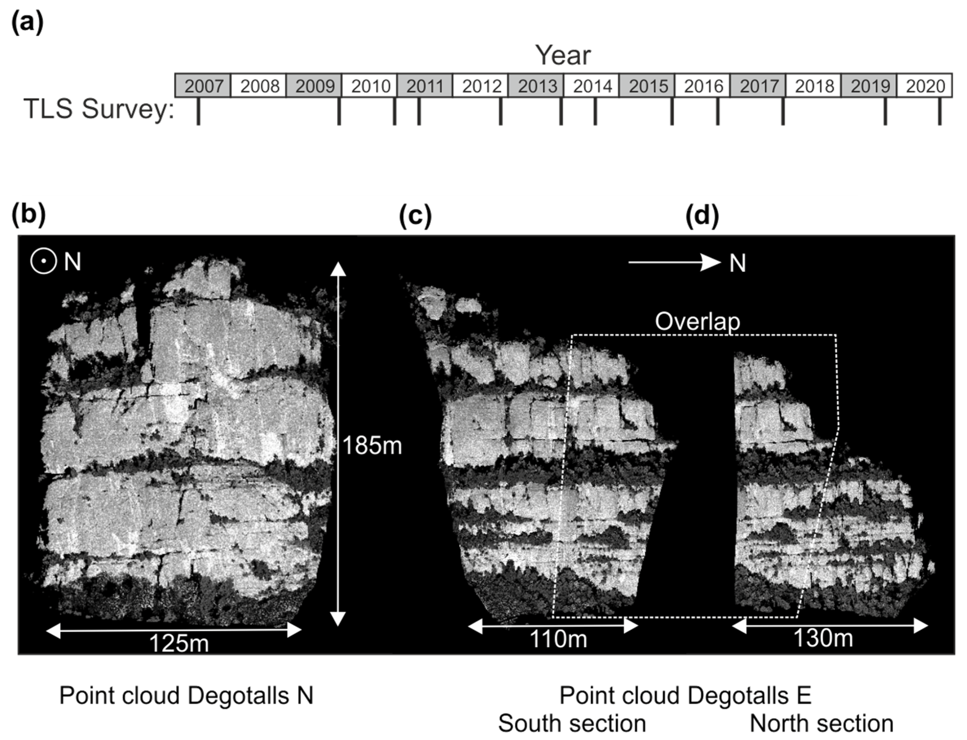
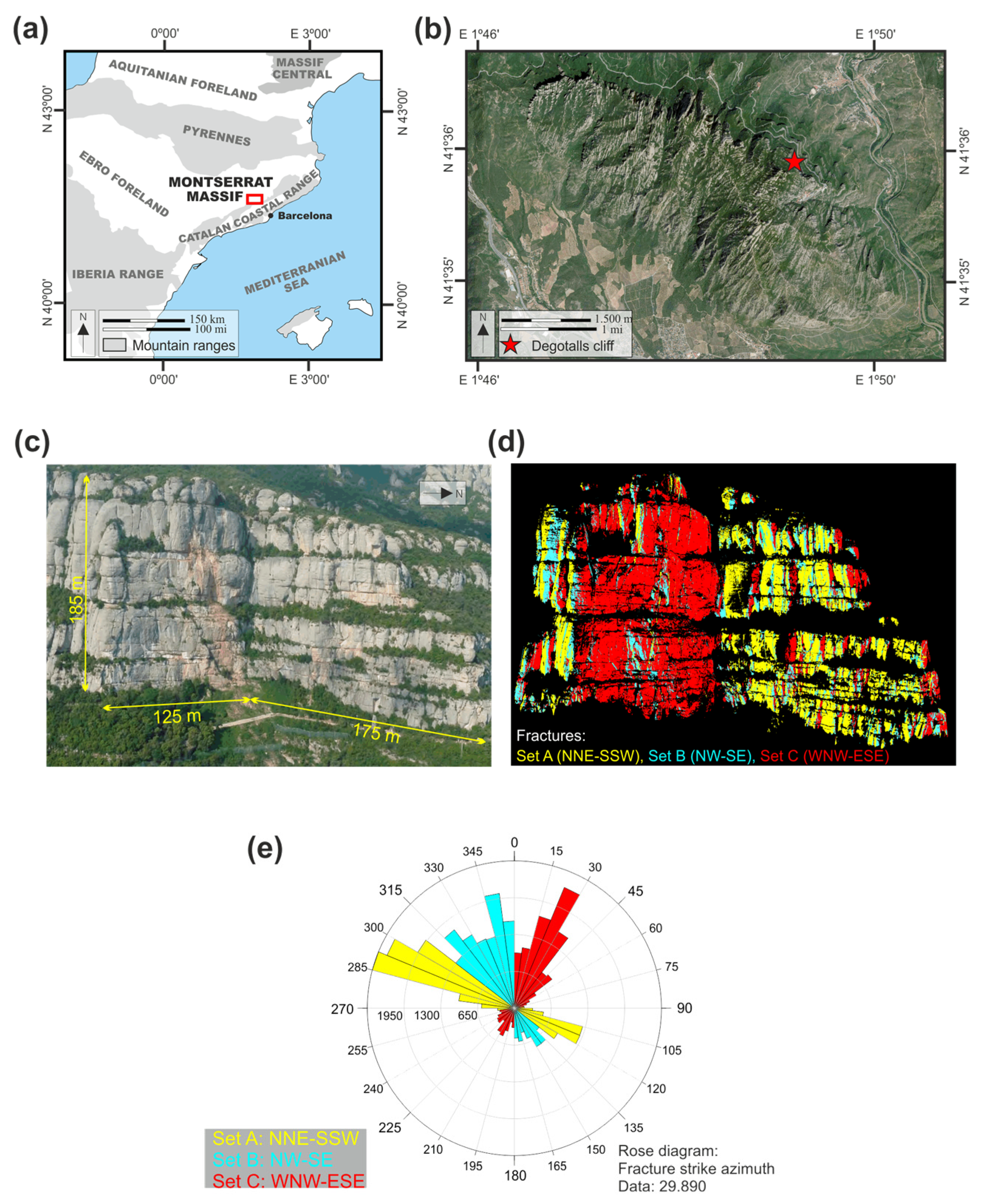
3. Study Sites and Processing

In this section, we detail the study sites and how the data has been collected and pre-processed.

Study Sites

The Montserrat massif is located about 40 km NW of Barcelona (Spain) with an extension of 35 km² with an elevation around 1000 m and a characteristic relief formed by rounded pinnacles and needles outlining many cliffs (see Figure 6a,b). The massif is a Natural Park and belongs to the Central Catalonia UNESCO Global Geopark as well as a tourist complex of cultural-religious heritage. The Montserrat sanctuary is located on the eastern part of the massif and attracts more than two million tourists and pilgrims per year. Thus, it requires large infrastructures, some of which are located next to cliffs with a high rockfall hazard. Precedents of rockfalls are numerous [20] all around the mountain, not excluding the sanctuary and the nearby Degotalls cliff (see Figure 6b,c).

Geologically, the massif consists of a succession of conglomerates (Montserrat conglomerates unit) more than 1000 m thick, interleaved by red siltstone and sandstone (La Salut and Artés Fm.) with sub-horizontal stratigraphic layers. The depositional system corresponds to a fan-delta complex accumulation in the Late-Eocene epoch along the southeastern margin of the Ebro Foreland Basin and adjacent to the Catalan Coastal Ranges [79,80,81].

A fracture pattern controls the morphology of the massif, with two orthogonal fracture sets oriented NNE-SSW (fracture set A) and WNW-ESE (fracture set C) [82] (as shown in Figure 6d,e). These sub-vertical, penetrative and high-frequency fracture sets cut the massif into blocks of decametric size, which together with the weathering action contribute to characterizing the peculiar landscape of the massif. The surface trace of the fractures can be followed for up to one kilometer on aerial photographs. Fracture set B with a NW-SE orientation has a lower frequency but contributes to the instability of the cliff, as well as its conjugate, with an NE-SW orientation and with a residual presence in the Degotalls area. The alphabetical order of the fracture sets defines their chronology from oldest to most recent [82]. Fractures represented in Figure 6d,e has been modeled with TLS data [83].

Due to the progressive event of rockfall failure that occurred in the North face of the Degotalls (hereafter Degotalls N) during the period 2001–2009 (see Figure 7) a risk mitigation plan was designed. In addition to protective measures, the plan triggered the monitoring of the Degotalls N and the orthogonal East face (hereafter Degotalls E) with TLS in 2007. The detachment of a high persistence fracture (fracture set C) and its fragmentation by the intersections with other fractures (fracture sets A and B) and stratigraphic layers resulted in rockfalls of decametric and metric dimensions.

Rockfalls at the Degotalls cliff are classified into three categories according to the instability mechanisms and the volume [20]: (a) large blocks, which are detachments of great volumes measuring several cubic meters and controlled by mechanical discontinuities produced by fractures and stratigraphic layers; (b) pebbles or pebble aggregates of medium to small volume, generally less than 1 m³, caused by detachments of the matrix due to weathering or associated with small fractures; and (c) plates, corresponding to weathering flakes and thermal exfoliation in slabs with small volumes (cm³ or dm³).

The monitoring system consists of 13 point cloud acquisitions with TLS Optech Ilris-3D (accuracy of σ = 0.7 cm at 100 m) [84] over the last 14 years, as details in Figure 8a from two different TLS stations. Degotalls N requires one scanner image acquisition (see Figure 8b), while Degotalls E requires two scanner images from another TLS station, designated as the first section (North) and the second section (South), respectively, as shown in Figure 8c,d. The range of the stations is about 175 m, and the height of the cliff is 185 m. The density of the scans is approximately one point each 7 cm, and the returned intensity of 1535 nm (infrared region) is recorded as a feature. In addition, high-resolution images were acquired to validate the “Candidate” class of clusters classified by the machine learning models.

A point cloud classification was executed to manually remove lush and easily identifiable vegetation, reducing uncertainty and facilitating the accuracy of the alignment process (see Figure 1). Degotalls scanner data were collected with point cloud format (Appendix A, with texture Intensity), measure differences (data output in Appendix B format) and clustering (data output in Appendix C format).

The data processing in the Degotalls cliffs was conducted with different strategies, the first objective being the identification of rockfalls and the second of previous deformation movements. The south section of Degotalls E cliff was compared throughout the monitoring period (2007–2020) with 12 consecutive comparisons, whereas the north section was performed with only one comparison for the same period. These different strategies of comparison are due to the reduced area of the north section and the need to identify previous deformation movements in the cliffs. Longer intervals are interpreted as sceneries more favorable to the identification of slow deformation movements. Otherwise, the Degotalls N cliff was compared in two batches, 2007–2017 and 2017–2020.

Throughout the monitoring period, point clouds were acquired from the same position, TLS device, and settings both for monitoring and calculation of the LoD of the system. Likewise, the differences between point clouds for this calibration were measured in areas with a perpendicular orientation to the TLS point position, without vegetation, and representative mean ranges to the cliff. In addition, the time interval between the calibration point clouds acquisition was 45 min. The dates of the point cloud acquisitions for monitoring are shown in Figure 8a.

4. Results

The parameters for the configuration of the double truncated cone and clustering are shown in

Table 6. Parameters to set the calibration and monitoring processes: (a) parameters used to define the geometry of the double truncated cone in the measure of the differences; (b) clustering parameters with the nomenclature equivalent to the DBSCAN algorithm; (c) mean and standard deviation to define the difference distribution for the TLS ILRIS-3D in both Degotalls areas for a mean range of 175 m.

(a) Distance Parameters	Degotalls Cliff (m)
Maximum vertical	0.5
Minimal horizontal	0.08
Maximal horizontal	0.10
(b) Clustering Settings
Threshold distance between points (eps)	0.15
Minimum number of points (minPts)	10 points
(c) Degotalls TLS System Calibration Difference
Mean	−0.000268
Standard deviation	0.019547

a,b. The values were fitted according to the resolution of the point cloud and the expected cluster sizes, generally present in the most frequent antecedents. Thereby, the metric of the differences is evaluated for fitting to a Gaussian distribution, and the statistical parameters of the mean and the standard deviation are computed (Table 6c).

Once the differences have been computed and the LoD established (see

Table 7. Statistical summary of the results of calculating the LoD in both Degotalls cliffs. This table summarizes the 13 comparisons in Degotalls E (12 in the South section and 1 in the North section) and 2 comparisons in Degotalls N.

Cliffs		LoD Mean (m)	LoD STD (m)
Degotalls E: South section	Upper	0.03242	0.00336
	Lower	−0.03189	0.00453
North section	Upper	0.03430	0.00590
	Lower	−0.03511	0.00385
Degotalls N:	Upper	0.03928	0.01685
	Lower	−0.04026	0.01626

), PCM software can the process the clustering of points step. From each monitoring the number of clusters in Degotalls E oscillates around 5800 in the South section, around 2600 in the North section, and around 3700 clusters in Degotalls N.

The monitoring dataset of the period 2007–2009 in the South section of Degotalls E is constituted by 5957 clusters. The training dataset was manually analyzed to identify 10 real rockfalls, labeled as “Candidates”, and 1990 other clusters labeled as “Unknown”. Thus, the Cluster Classification pipeline (see flowchart in Figure 5) begins with the training stage with 1990 clusters from the “Unknown” class and 10 clusters from the “Candidate” class. The pipeline combines the 15 resampling techniques (shown in Table 3) with the 11 classification models (shown in Table 4) using 10-fold cross-validation procedure, after normalizing the dataset fitting 165 classification configurations (i.e., 15 resampling techniques times 11 classification models). Thereafter, trained models were used as predictive models with the rest of the 3957 unclassified clusters (test dataset with 5957 initial clusters, less 10 clusters “Candidate” and 1990 from the “Unknown” class) from the period 2007–2009 in order to identify new “Candidate” clusters.

The clusters labeled as “Candidate” by the 165 predictive configurations of the models were validated manually together with the 3957 clusters of the period 2007–2009, thereby identifying eight new rockfalls. Metric evaluation of the best predictive and the resampling model is shown in

Table 8. Summary of the predictive models results in the Degotalls where the disparity of the best methods is appreciated attending to the true positive (TP), false positive (FP), and false negative (FN) results. Degotalls N presents two solutions: ^a the best solution with false negatives = 0 or ^b the best solution, but accepting a reduced number of false negatives. * Initial manual classification. Clusters of “Rockfalls for training” are referred to in the “Candidate” class in the training stage. Real rockfall is referred to existent and known rockfalls on the bedrock.

Outcrop Period	Rockfalls for Training	Best Classifier Model	Best Resampling Method	Real Rockfalls	TP	FP	FN
Degotalls E South section
2007–2009	10 *	Quadratic Discr.	Pol. Fit-SMOTE	8	8	91	0
2009–2010	18	Linear Discr. A.	Cluster Centr.	5	5	7	0
2010–2011	23	KNN C.	Cluster Centr.	4	4	139	0
2011–2012	27	XGBoost C.	S. TomekLinks	4	4	48	0
2012–2013	31	Extra Trees C.	Cluster Centr.	2	2	10	0
2013–2014	33	XGBoost C.	Cluster Centr.	1	1	1	0
2014–2015	34	SVC	Cluster Centr.	1	1	0	0
2015–2016	35	Linear Discr. A.	Stefanowsky	3	3	53	0
2016–2017	38	-	-	0
2017–2019	38	Linear Discr. A.	Cluster Centr.	3	3	9	0
2019–2020	41	-	-	0
2020–2020	41	Extra Trees C.	Stefanowsky	2	2	2	0
North section
2007–2019	43	Quadratic Discr.	LVQ-SMOTE	22	22	97	0
Degotalls N
2007–2017 a	10 *	Linear Discr. A.	Cluster Repres.	107	107	1211	0
2007–2017 b	10	Decision Tree C.	Cluster Repres.	107	104	296	3
2017–2019 a	117	Quadratic Discr.	SWIM	16	16	455	0
2017–2019 b	117	Quadratic Discr.	Pro WSyn	16	15	256	1

and

Table 9. Summary of the metric for the predictive models results with Recall and Accuracy parameters. Degotalls N presents two solutions: ^a the best solution with False Negatives = 0 or ^b the best solution, but accepting a reduced number of False Negatives.

Outcrop Period	Best Classifier Model	Best Resampling Method	Recall	Accuracy
Degotalls E South section
2007–2009	Quadratic Discr.	Pol. Fit-SMOTE	1	0.979
2009–2010	Linear Discr. A.	Cluster Centr.	1	0.999
2010–2011	KNN C.	Cluster Centr.	1	0.979
2011–2012	XGBoost C.	S. TomekLinks	1	0.991
2012–2013	Extra Trees C.	Cluster Centr.	1	0.998
2013–2014	XGBoost C.	Cluster Centr.	1	0.999
2014–2015	SVC	Cluster Centr.	1	1
2015–2016	Linear Discr. A.	Stefanowsky	1	0.992
2016–2017	-	-
2017–2019	Linear Discr. A.	Cluster Centr.	1	0.998
2019–2020	-	-
2020–2020	Extra Trees C.	Stefanowsky	1	0.999
North section
2007–2019	Quadratic Discr.	LVQ-SMOTE	1	0.968
Degotalls N
2007–2017 a	Linear Discr. A.	Cluster Repres.	1	0.704
2007–2017 b	Decision Tree C.	Cluster Repres.	0.972	0.906
2017–2019 a	Quadratic Discr.	SWIM	1	0.891
2017–2019 b	Quadratic Discr.	Pro WSyn	0.937	0.935

(Degotalls E, south section, 2007–2009).

Classification of the following monitoring period (2009–2010) uses the 18 validated candidates (10 + 8) and the totality of the unknown clusters from the 2007–2009 monitoring for the training stage. When it finalizes, 165 configurations of the models are fitted again to be used as predictive models with the 5100 “Unknown” clusters for the period 2009–2010. The new cluster “Candidate” proposed by the predictive models are validated again with high-resolution images and their metrics evaluated. This procedure is repeated until completion of the monitoring period and showed in Table 8, Degotalls E, South section.

The Degotalls E North section begins the learning stage with the 43 clusters labeled as “Candidate” from the South section in order to analyze one comparison monitoring of the period 2007–2019. The aim was to identify pre-deformation movements and rockfall clusters, although only 22 validated “Candidate” of rockfalls were identified (as shown in Table 8, Degotalls E, North section) and none of pre-deformation.

The Degotalls N pipeline was initialized with the manual identification of the new 10 rockfall clusters for the analysis of two comparison monitoring periods 2007–2017 and 2017–2019. The search for pre-deformation movement clusters was also negative. The results are shown in Table 8 and Table 9, Degotalls N.

With the increase in the number of clusters labeled as “Candidate”, the Degotalls E South section dataset tends to decrease the number of false positives. Nevertheless, although the metric of the best classifier and resampling models reveal a high percentage of models with optimal results (Table 8). It is observed that the best classifier and resampling models are different for each comparison.

The manual cluster validation of the predictive results demonstrates the existence, especially in Degotalls E, of acceptable results in terms of true positives, false positives, and false negatives. It should be noted that the number of initial clusters for each monitoring is around 5000–6000. However, after the classification of the predictive models, there is a significant reduction in the number of clusters to be validated. Degotalls N presents an elevated number of false positives, especially when total identification of TP success is required for the results for the real number of rockfalls.

Table 10. Quadratic discriminant analysis model and polynom-fit-SMOTE resampling results. This combination shows the best model for the 2007–2009 comparison, but not for the following comparison in true positive (TP), false positive (FP) and false negative (FN) results.

Outcrop Period	Real Rockfalls	TP	FP	FN
Degotalls E South section
2007–2009	8	8	91	0
2009–2010	5	5	148	0
2010–2011	4	4	461	0
2011–2012	4	4	258	0
2012–2013	2	2	235	0
2013–2014	1	1	224	0
2014–2015	1	1	188	0
2015–2016	3	3	315	0
2016–2017	0	-	-	-
2017–2019	3	2	517	1
2019–2020	0	-	-	-
2020–2020	2	2	111	0

shows the example when the first best predictive model of the first comparison in Degotalls E (i.e., quadratic discriminant analysis and polynom-fit-SMOTE) is used for the whole period. The results are not acceptable due to a large number of false positives and therefore, the large number of cluster candidates to be validated. Neither is observed a clear tendency to reduce FP.

However, there are correct identifications among the 165 configurations of the models (see Table 8), and above all the percentage of these configurations with TP is significant. It is difficult to select one model as the best one, the common practice in the machine learning field is to use a pipeline of models and perform cross-validation and to select the one or ones that obtain the performance (based on accuracy or recall, for example).

To solve this problem, we seek to validate only the clusters labeled as “Candidate” which were proposed by the totality of the predictive models to most improve the score. With this premise, the “Candidate” labeled clusters validated manually as rockfalls or true positives clusters in Degotalls E are always among the 115 clusters most predicted by the models. An initial average survey of 5800 clusters belonging to the “Unknown” class produced by each monitoring period, reveal a reduction of 98% in the number of clusters to be validated (true positives and false positives) with real rockfalls from the rock cliff (true positives). In Degotalls N the reduction in “Candidate” clusters to be validated is 80.16% for complete identification of rockfalls, and in order to identify 96% of the real rockfalls, the reduction is 90% from a population of 3700 initial class of “Unknown” clusters.

Figure 9 depicts one example of cluster validation, comparing the cluster images of one cluster before and after the monitoring, and visualizing the cluster features. The feature clusters are shown in

Table 11. Summary of features of the cluster shown in Figure 9. Cluster #1326 (Degotalls E, south section, period 2017–2019).

Cluster Feature	Value	Cluster Feature	Value
Cluster Number	1326	Points %: Noise	10.48%
Centroid Coord. X	−23.169 m	Advance	0.21%
Coord. Y	192.847 m	Retreat	89.31%
Coord. Z	−10.063 m	Intensity Ref.	210.32
Number of points	428	Intensity Comp.	228.43
Positive Volume	0.27164 m3	Azimuth Ref.	165.10°
Area	1.45 m2	Azimuth Comp.	166.20°
Predominance: Mean	2 (Retreat)	Slope Ref.	71.11°
Standard deviation	0.07	Slope Comp.	70.91°

.

The total number of clusters labeled as “Candidate” and validated as rockfall events at Degotalls E during the monitoring period was 65. At Degotalls N the number of candidates validated was 133, but 40 clusters of them correspond in fact, to only two large events occurred in December of 2008, therefore we assess 95 rockfalls (see Figure 10). This re-count is due to the configuration of the monitoring process focused on preventing the loss of small rockfalls. The number of events registered using the standard methodology [20,57] is also shown in Figure 10.

5. Discussion

In this study, an inventory of rockfalls is constructed from point clouds with two new methods (PCM and Cluster Classification). PCM software is implemented to characterize and identify clusters of differences during monitoring processes, and Cluster Classification software classifies the nature of the clusters. Specifically, it is trained to classify clusters of rockfalls with machine learning techniques. The inventory was created covering the period 2007–2020 for the Degotalls cliff area (Montserrat massif, Spain). The cliff, divided into Degotalls E and Degotalls N, accounts for 65 and 95 rockfalls, respectively, and these results are adjusted to the expected and known values of the previous studies in the area [20,57].

PCM software calculates the LoD (as shown in Table 7), and the order of magnitude of the results are similar to those used previously in the monitoring of the Degotalls and recommended in previous works [20,57]. In general, values of the LoD in Degotalls N are higher (20%) than those in Degotalls E, but this is attributable to the greatest height of the Degotalls N cliff, and therefore, with a somewhat greater TLS–cliff distance.

Measure differences and clustering points are integrated processes in PCM software and offer similar results to previous studies conducted in the area with the M3C2 and DBSCAN algorithms by Royán et al. [57] and Janeras et al. [20]. PCM software complements results with features that characterize firstly the points and subsequently, the clusters (e.g., predominance, coplanarity, or normal vector) to feed the machine learning classification process.

The results of cluster classification provide differences in the number of rockfalls counted with respect to previous works, but this fact is attributable to the different methods of validation. In this work, only those clusters labeled as “Candidate” with a clear validation in high-resolution images have been accepted. The disparate results of the predictive models for both scenarios have been interpreted in Degotalls E as promising, which opens up the possibility of studying in greater detail the importance of each feature in the contribution of the models. Moreover, this can be extended to the study of the efficiency of each resample technique and each classification model to evolve the identification of deformation clusters. At Degotalls E, the manual validation of the first 16 clusters labeled as “Candidate” most frequently proposed by the 165 predictive models identifies 65% of the rockfalls. If the manual validation is extended to the first 115 cluster candidates, the identification reaches 100% of the rockfalls. This implies a significant reduction in the initial clusters to validate them as rockfalls. The efficiency of predictive models also tends to increase when the rockfall database increases in number with new identifications in future monitoring.

Otherwise, the results from Degotalls N, with a higher percentage of clusters to be validated, the 370 clusters labeled as “Candidate” to identify 90% of the rockfalls show the potential for further improvement focused on reducing this percentage.

The analysis of these validated clusters reveals a relationship between the feature volume and the ratio of real TP identifications of the predictive models. The predictive models have a lower percentage of real TP identifications with large volume rockfalls (see Figure 11a), while in Degotalls E (shown in Figure 11b) large blocks are not presents. Degotalls N presents the clusters labeled as “Candidate” least predicted by the models belonging mainly to the category of large blocks, with volumes greater than 0.1 m³. On the other hand, the clusters corresponding to the category of plates with smaller volumes obtain the highest levels of real TP identifications in the prediction because they present more homogeneous characteristics and, therefore, facilitate the training.

Clusters of rockfalls in Degotalls N can be regarded heterogeneous (in terms of features: e.g., volume, orientation, intensity), and therefore are more difficult to learn in the training stage since the characteristics of the clusters are not as polarized as in Degotalls E. The two largest-volume clusters in Degotalls N have the lowest percentage of model predictions because they have a high degree of singularity, which does not contribute to defining a homogeneous class for the model learning. An increase in rockfalls in the dataset collection may correct this problem, but it is difficult to increase ratio between the number of “Candidate” and “Unknown” along the time with the current scenarios.

The large blocks (>1 m³) category was predominant in Degotalls N during the first two years of monitoring, and were associated with the large event controlled by fractures in 2001 and their subsequent risk mitigation activities, as it can be seen in Figure 7. In the second stage, both rock cliffs enter a stability period in which a reduced and constant number of rockfalls belonging to the category plates predominated, linked to the lingering weathering process. In Degotalls E, we observed some detachments of small volumes with some events controlled by fractures around the cubic meter of volumes. The increase in registered events in both rock cliffs (look at Figure 10) since 2018 corresponds to the category plates with small volumes (see Figure 11) of less than half a cubic meter.

The cumulative distribution of volumes registered in the Degotalls presents slightly different power law exponents in both cliffs, despite the fact that the rock mass structural conditions are the same, except rock face orientation. In the case of Degotalls N, the distribution covers a wider range of orders of magnitude due to the 2007–2009 large rockfalls event (see Figure 12). In consequence, the common sample in the range of 0.01 to 10 m³ is the most representative of the rockfall activity that we are clearly detecting with TLS in the Degotalls area. These results should determine the scenarios to be considered in further hazard assessment for the sanctuary parking area [85].

A possible new strategy to optimize the results in Degotalls N is to feed the training stage with each different category (large block, pebble, and plate), but always considering a significant number of “Candidate” labeled clusters.

On comparison with the results from the standard methodology in the Degotalls [20,57], a variation is found to exist in the amount and temporal distribution of the events. This can undoubtedly be attributed to the reduction in the number of clusters to be validated allowing an increase in the quality of the validation that reduces doubtful cases. Furthermore, the objective assessment of each cluster as a candidate for a rockfall improves the process, and contributes to a better interpretation of the rock cliff evolution and the valuation of risk mitigation activities.

Analysis of the nature of the clusters has been unable to identify any pre-deformation process with which to create a new class. The study of the area in years prior to the rockfall has been unproductive. The reason for this non-identification may be due to using a temporal resolution that is too low to record this process. Possibly, the modification of the temporal and spatial resolution during the monitoring allows the identification of pre-deformed clusters, and therefore enables their classification with our methodology.

The time required to process the measure differences process may constitute a limitation of the process, even though it is an automatic process. Several factors are involved in controlling this step, and it may be convenient to minimize this time.

6. Conclusions

Monitoring rock cliffs to identify rockfalls with point clouds requires dataset processing methods, many of which are developed by the research community. Periodic digital capture of cliff surfaces with instruments such as TLS does not directly provide an inventory of rockfalls. For this aim, it is necessary to process the captured data and configure the temporal and spatial resolutions of the TLS in accordance with the dynamics of the rockfalls from the cliff. The capture of point clouds, their alignment, the measure of the differences, and the clustering are more highly evolved aspects. However, classification of the clusters is a factor that is not so frequently addressed. The present work proposes a solution to this issue based on machine learning and predictive models.

In this paper, we propose two developments, PCM and Cluster Classification applications, to automatically classify clusters with machine learning by taking advantage of the fact that clusters that contain rockfalls have similar characteristics, a fact that facilitates the learning stage. As observed in Degotalls N, singular rockfalls (those covering large volumes) are the most complicated to learn. The proposed modifications of the already existing algorithms that deal with the creation of clusters have been very useful for measure 33 features especially significant during the classification. However, the discrimination power of each feature introduced in the learning process has not been tested in this work, an issue that should be addressed in future studies.

The machine learning process implies the development of 165 prediction models based on the 11 classification models, combined with 15 resampling methods (13 undersampling and 2 oversampling) to balance the unbalances between the number of clusters in the rockfall class of the non-rockfall class. A total of 11 classification models have used the balanced data to classify the rockfalls class using 10-fold cross-validation and hyper-parameterization techniques.

In summary, the following conclusions are derived from this work:

-

Monitoring rockfalls in rock cliffs with point cloud is a difficult task that can benefit from machine learning strategies, provided that both techniques are appropriately combined. We validate this assumption with the attempt to identify rockfalls in the rock cliff of the Montserrat massif (Spain).

-

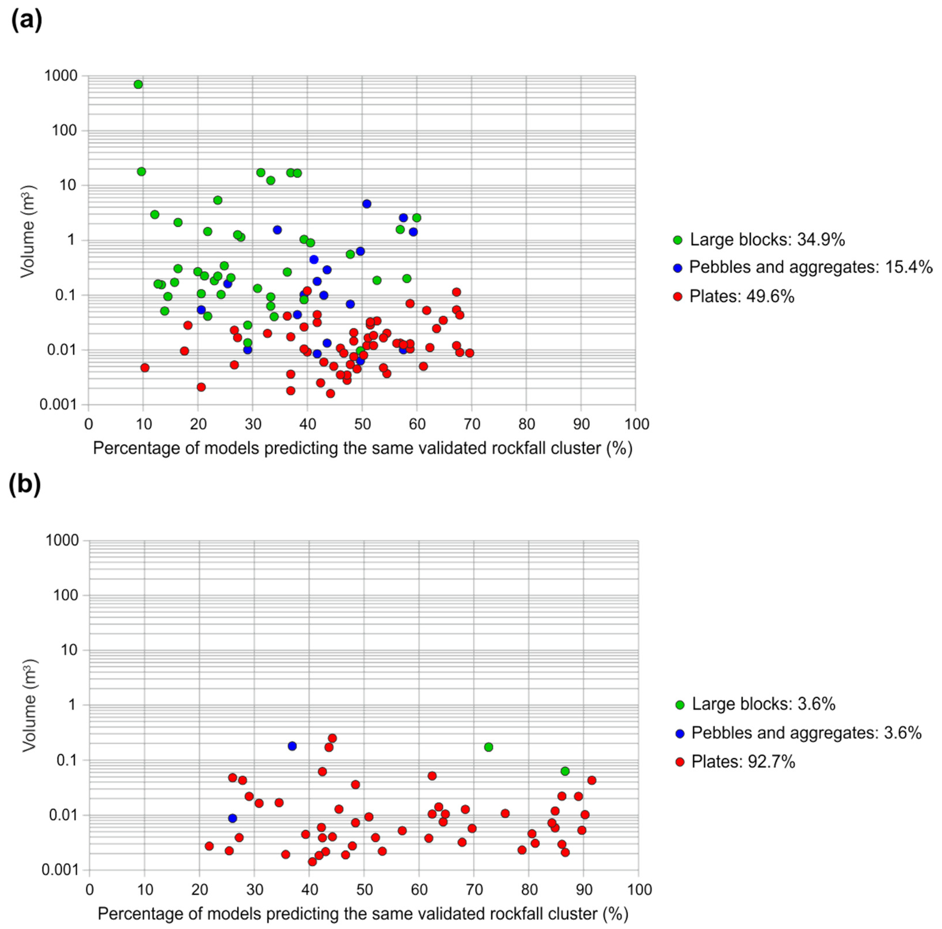
We have observed the difficulty of correlating classification models, trained with clusters of rockfalls, with the best prediction model. For this reason, we use all the combinations of prediction models to validate the most proposed candidates.

-

The success of the rockfall prediction models depends on the homogeneity/heterogeneity of the features that characterize the different categories of the rockfall clusters (large blocks, pebbles and plates) used to train the classification models.

-

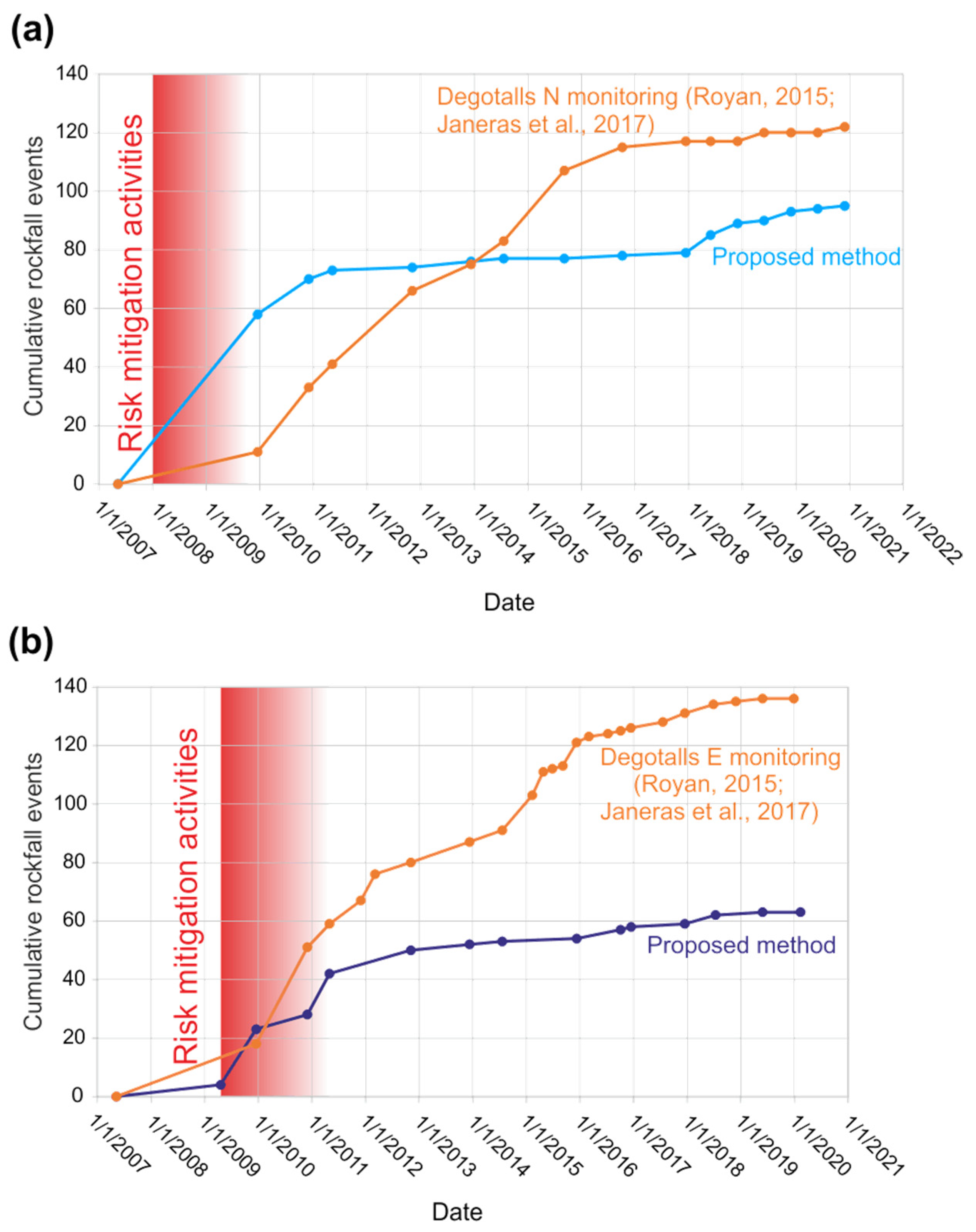
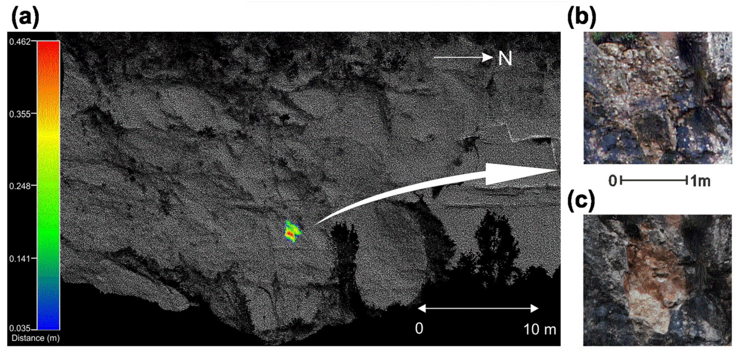
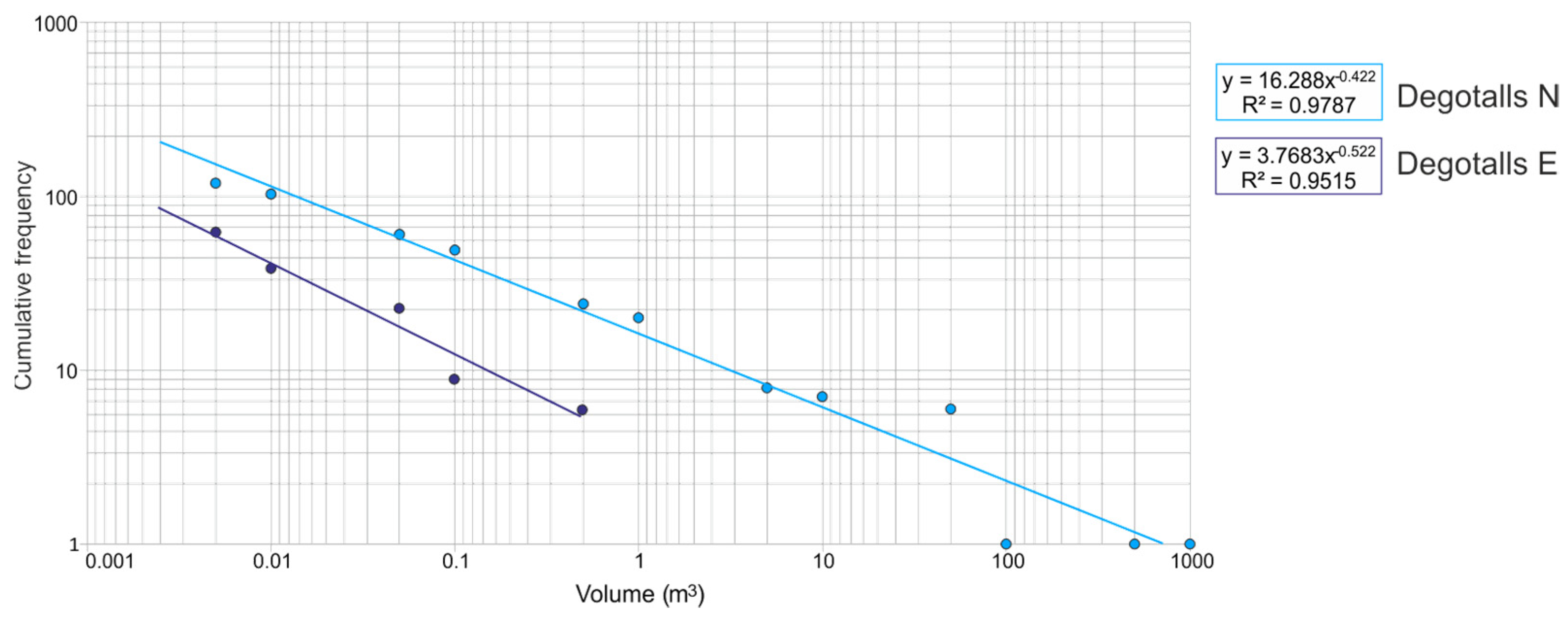
Rockfalls in the Degotalls (Montserrat, Spain) are currently in a phase of stabilization, and those that occur are of small volume and attributable to plates associated with weathering processes. However, since 2018 a slight increase in cases has been observed.

References

1. Erismann, T.H.; Abele, G. Dynamics of Rockslides and Rockfalls; Springer: Berlin/Heidelberg, Germany, 2001; ISBN 978-3-642-08653-3. [Google Scholar]
2. Whalley, W.B. Rockfalls. In Slope Instability; Brunsden, D., Prior, D.B., Eds.; Wiley: Chichester, UK, 1984; pp. 217–256. [Google Scholar]
3. Hungr, O.; Leroueil, S.; Picarelli, L. The Varnes Classification of Landslide Types, an Update. Landslides 2014, 11, 167–194. [Google Scholar] [CrossRef]
4. DiFrancesco, P.-M.; Bonneau, D.; Hutchinson, D.J. The Implications of M3C2 Projection Diameter on 3D Semi-Automated Rockfall Extraction from Sequential Terrestrial Laser Scanning Point Clouds. Remote Sens. 2020, 12, 1885. [Google Scholar] [CrossRef]
5. Volkwein, A.; Schellenberg, K.; Labiouse, V.; Agliardi, F.; Berger, F.; Bourrier, F.; Dorren, L.K.A.; Gerber, W.; Jaboyedoff, M. Rockfall Characterisation and Structural Protection—A Review. Nat. Hazards Earth Syst. Sci. 2011, 11, 2617–2651. [Google Scholar] [CrossRef]
6. Corominas, J.; Copons, R.; Moya, J.; Vilaplana, J.M.; Altimir, J.; Amigó, J. Quantitative Assessment of the Residual Risk in a Rockfall Protected Area. Landslides 2005, 2, 343–357. [Google Scholar] [CrossRef]
7. van Veen, M.; Hutchinson, D.J.; Kromer, R.; Lato, M.; Edwards, T. Effects of Sampling Interval on the Frequency—Magnitude Relationship of Rockfalls Detected from Terrestrial Laser Scanning Using Semi-Automated Methods. Landslides 2017, 14, 1579–1592. [Google Scholar] [CrossRef]
8. Williams, J.G.; Rosser, N.J.; Hardy, R.J.; Brain, M.J. The Importance of Monitoring Interval for Rockfall Magnitude-Frequency Estimation. J. Geophys. Res. Earth Surf. 2019, 124, 2841–2853. [Google Scholar] [CrossRef]
9. Ritchie, A.M. Evaluation of Rockfall and Its Control. Highw. Res. Rec. 1963, 17, 13–28. [Google Scholar]
10. Sturzenegger, M.; Stead, D. Quantifying Discontinuity Orientation and Persistence on High Mountain Rock Slopes and Large Landslides Using Terrestrial Remote Sensing Techniques. Nat. Hazards Earth Syst. Sci. 2009, 9, 267–287. [Google Scholar] [CrossRef]
11. Abellán, A.; Oppikofer, T.; Jaboyedoff, M.; Rosser, N.J.; Lim, M.; Lato, M.J. Terrestrial Laser Scanning of Rock Slope Instabilities. Earth Surf. Process. Landf. 2014, 39, 80–97. [Google Scholar] [CrossRef]
12. Abellan, A.; Derron, M.-H.; Jaboyedoff, M. “Use of 3D Point Clouds in Geohazards” Special Issue: Current Challenges and Future Trends. Remote Sens. 2016, 8, 130. [Google Scholar] [CrossRef]
13. Telling, J.; Lyda, A.; Hartzell, P.; Glennie, C. Review of Earth Science Research Using Terrestrial Laser Scanning. Earth Sci. Rev. 2017, 169, 35–68. [Google Scholar] [CrossRef] [Green Version]
14. Santana, D.; Corominas, J.; Mavrouli, O.; Garcia-Sellés, D. Magnitude–Frequency Relation for Rockfall Scars Using a Terrestrial Laser Scanner. Eng. Geol. 2012, 145–146, 50–64. [Google Scholar] [CrossRef]
15. Corominas, J.; Mavrouli, O.; Ruiz-Carulla, R. Rockfall Occurrence and Fragmentation. In Advancing Culture of Living with Landslides; Springer International Publishing: Cham, Switzerland, 2017; pp. 75–97. [Google Scholar] [CrossRef]
16. Fanti, R.; Gigli, G.; Lombardi, L.; Tapete, D.; Canuti, P. Terrestrial Laser Scanning for Rockfall Stability Analysis in the Cultural Heritage Site of Pitigliano (Italy). Landslides 2013, 10, 409–420. [Google Scholar] [CrossRef]
17. Mazzanti, P.; Schilirò, L.; Martino, S.; Antonielli, B.; Brizi, E.; Brunetti, A.; Margottini, C.; Scarascia Mugnozza, G. The Contribution of Terrestrial Laser Scanning to the Analysis of Cliff Slope Stability in Sugano (Central Italy). Remote Sens. 2018, 10, 1475. [Google Scholar] [CrossRef]
18. Lague, D.; Brodu, N.; Leroux, J. Accurate 3D Comparison of Complex Topography with Terrestrial Laser Scanner: Application to the Rangitikei Canyon (N-Z). ISPRS J. Photogramm. Remote Sens. 2013, 82, 10–26. [Google Scholar] [CrossRef]
19. Tonini, M.; Abellán, A. Rockfall Detection from Terrestrial Lidar Point Clouds: A clustering approach using R. J. Spat. Inf. Sci. 2013, 8, 95–110. [Google Scholar] [CrossRef]
20. Janeras, M.; Jara, J.-A.; Royán, M.J.; Vilaplana, J.-M.; Aguasca, A.; Fàbregas, X.; Gili, J.A.; Buxó, P. Multi-technique Approach to Rockfall Monitoring in the Montserrat Massif (Catalonia, NE Spain). Eng. Geol. 2017, 219, 4–20. [Google Scholar] [CrossRef]
21. Bonneau, D.; DiFrancesco, P.M.; Jean Hutchinson, D. Surface Reconstruction for Three-Dimensional Rockfall Volumetric Analysis. ISPRS Int. J. Geo-Inf. 2019, 8, 548. [Google Scholar] [CrossRef]
22. Bonneau, D.A.; Hutchinson, D.J. The Use of Terrestrial Laser Scanning for the Characterization of a Cliff-Talus System in the Thompson River Valley, British Columbia, Canada. Geomorphology 2019, 327, 598–609. [Google Scholar] [CrossRef]
23. Hendrickx, H.; Le Roy, G.; Helmstetter, A.; Pointner, E.; Larose, E.; Braillard, L.; Nyssen, J.; Delaloye, R.; Amaury, F. Timing, Volume and Precursory Indicators of Rock and Cliff Fall on a Permafrost Mountain Ridge (Mattertal, Switzerland). Earth Surf. Process Landf. 2022, 47, 1532–1549. [Google Scholar] [CrossRef]
24. Rosser, N.; Lim, M.; Petley, D.; Dunning, S.; Allison, R. Patterns of Precursory Rockfall Prior to Slope Failure. J. Geophys. Res. 2007, 112, 148–227. [Google Scholar] [CrossRef]
25. Kromer, R.; Hutchinson, D.; Lato, M.; Gauthier, D.; Edwards, T. Identifying Rock Slope Failure Precursors Using LiDAR for Transportation Corridor Hazard Management. Eng. Geol. 2015, 195, 93–103. [Google Scholar] [CrossRef]
26. Carrea, D.; Abellan, A.; Derron, M.H.; Jaboyedoff, M. Automatic Rockfalls Volume Estimation Based on Terrestrial Laser Scanning Data. In Engineering Geology for Society and Territory—Volume 2: Landslide Processes; Springer International Publishing: Cham, Switzerland, 2015; pp. 425–428. ISBN 9783319090573. [Google Scholar]
27. Blanch, X.; Eltner, A.; Guinau, M.; Abellan, A. Multi-Epoch and Multi-Imagery (MEMI) Photogrammetric Workflow for Enhanced Change Detection Using Time-Lapse Cameras. Remote Sens. 2021, 13, 1460. [Google Scholar] [CrossRef]
28. Kromer, R.; Walton, G.; Gray, B.; Lato, M.; Group, R. Development and Optimization of an Automated Fixed-Location Time Lapse Photogrammetric Rock Slope Monitoring System. Remote Sens. 2019, 11, 1890. [Google Scholar] [CrossRef]
29. Williams, J.; Rosser, N.J.; Hardy, R.; Brain, M.; Afana, A. Optimising 4-D Surface Change Detection: An Approach for Capturing Rockfall Magnitude–Frequency. Earth Surf. Dyn. 2018, 6, 101–119. [Google Scholar] [CrossRef]
30. Schovanec, H.; Walton, G.; Kromer, R.; Malsam, A. Development of Improved Semi-Automated Processing Algorithms for the Creation of Rockfall Databases. Remote Sens. 2021, 13, 1479. [Google Scholar] [CrossRef]
31. Eberhardt, E.; Stead, D.; Coggan, J.S. Numerical Analysis of Initiation and Progressive Failure in Natural Rock Slopes—the 1991 Randa Rockslide. Int. J. Rock Mech. Min. Sci. 2004, 41, 69–87. [Google Scholar] [CrossRef]
32. Zoumpekas, T.; Puig, A.; Salamó, M.; García-Sellés, D.; Blanco-Nuñez, L.; Guinau, M. An Intelligent framework for End-to-End Rockfall Detection. Int. J. Intell. Syst. 2021, 36, 6471–6502. [Google Scholar] [CrossRef]
33. Weidner, L.; Walton, G.; Kromer, R. Classification Methods for Point Clouds in Rock Slope Monitoring: A Novel Machine Learning Approach and Comparative Analysis. Eng. Geol. 2019, 263, 105326. [Google Scholar] [CrossRef]
34. Brodu, N.; Lague, D. 3D Terrestrial Lidar Data Classification of Complex Natural Scenes Using a Multi-Scale Dimensionality Criterion: Applications in Geomorphology. ISPRS J. Photogramm. Remote Sens. 2012, 68, 121–134. [Google Scholar] [CrossRef] [Green Version]
35. Zhang, W.; Qi, J.; Wan, P.; Wang, H.; Xie, D.; Wang, X.; Yan, G. An Easy-to-Use Airborne LiDAR Data Filtering Method Based on Cloth Simulation. Remote Sens. 2016, 8, 501. [Google Scholar] [CrossRef]
36. Evans, J.S.; Hudak, A.T. A Multiscale Curvature Algorithm For Classifying Discrete Return LiDAR in Forested Environments. IEEE Trans. Geosci. Remote Sens. 2007, 45, 1029–1038. [Google Scholar] [CrossRef]
37. Kromer, R.; Lato, M.; Hutchinson, D.J.; Gauthier, D.; Edwards, T. Managing Rockfall Risk through Baseline Monitoring of Precursors Using a Terrestrial Laser Scanner. Can. Geotech. J. 2017, 54, 953–967. [Google Scholar] [CrossRef]
38. Mazzanti, P.; Caporossi, P.; Brunetti, A.; Mohammadi, F.I.; Bozzano, F. Short-Term Geomorphological Evolution of the Poggio Baldi Landslide Upper Scarp via 3D Change Detection. Landslides 2021, 18, 2367–2381. [Google Scholar] [CrossRef]
39. Royán, M.J.; Abellán, A.; Jaboyedoff, M.; Vilaplana, J.M.; Calvet, J. Spatio-Temporal Analysis of Rockfall Pre-Failure Deformation Using Terrestrial LiDAR. Landslides 2014, 11, 697–709. [Google Scholar] [CrossRef]
40. Ester, M.; Kriegel, H.-P.; Sander, J.; Xu, X. A Density-Based Algorithm for Discovering Clusters in Large Spatial Databases with Noise. In Proceedings of the Second International Conference on Knowledge Discovery and Data Mining, Portland, OR, USA, 2–4 August 1996; Simoudis, E., Fayyad, U., Han, J., Eds.; AAAI Press: Menlo Park, CA, USA, 1996; pp. 226–231. [Google Scholar]
41. Girardeau-Montaut, D.; Roux, M.; Marc, R.; Thibault, G. Change Detection on Points Cloud Data Acquired with a Ground Laser scanner. In Proceedings of the ISPRS WG III/3, III/4, V/3Workshop “Laser Scanning 2005”, Enschede, The Netherlands, 12–14 September 2005; Vosselman, G., Brenner, C., Eds.; 2005; pp. 30–35. Available online: https://www.isprs.org/proceedings/xxxvi/3-w19/ (accessed on 21 June 2022).
42. Innovmetric. Polyworks. Quebec City. 2022. Available online: https://www.innovmetric.com (accessed on 18 May 2022).
43. Visual Studio 2019. Microsoft. Available online: https://Visualstudio.microsoft.com (accessed on 18 May 2022).
44. Barnhart, T.B.; Crosby, B.T. Comparing TwoMethods of Surface Change Detection on an Evolving Thermokarst Using High-Temporal-Frequency Terrestrial Laser Scanning, Selawik River, Alaska. Remote Sens. 2013, 5, 2813–2837. [Google Scholar] [CrossRef]
45. Cignoni, P.; Rocchini, C.; Scopigno, R. Metro: Measuring Error on Simplified Surfaces. Comput. Graph. Forum 1998, 17, 167–174. [Google Scholar] [CrossRef]
46. Kazhdan, M.; Bolitho, M.; Hoppe, H. Poisson Surface Reconstruction. In Eurographics Symposium on Geometry Processing; Sheffer, A., Poithier, K., Eds.; The Eurographics Association, 2006; Available online: http://diglib.eg.org/handle/10.2312/SGP.SGP06.061-070 (accessed on 18 May 2022).
47. Girardeu-Montaut, D. CloudCompare, Version 2.12.1 Alpha. Available online: http://www.cloudcompare.org/ (accessed on 18 May 2022).
48. Abellán, A.; Jaboyedoff, M.; Oppikofer, T.; Vilaplana, J.M. Detection of Millimetric Deformation Using a Terrestrial Laser Scanner: Experiment and Application to a Rockfall Event. Nat. Hazards Earth Syst. Sci. 2009, 9, 365–372. [Google Scholar] [CrossRef]
49. Jolliffe, I. Principal Component Analysis. In International Encyclopedia of Statistical Science; Springer: Berlin/Heidelberg, Germany, 2011. [Google Scholar] [CrossRef]
50. Woodcock, N. Specification of fabric shapes using an Eigenvalue method. Geol. Soc. Am. Bull. 1977, 88, 1231–1236. [Google Scholar] [CrossRef]
51. García-Sellés, D.; Falivene, O.; Arbués, P.; Gratacós, O.; Tavani, S.; Muñoz, J.A. Supervised Identification and Reconstruction of Near-Planar Geological Surfaces from Terrestrial Laser Scanning. Comput. Geosci. 2011, 37, 1584–1594. [Google Scholar] [CrossRef]
52. Benjamin, J.; Rosser, N.J.; Brain, M.J. Emergent Characteristics of Rockfall Inventories Captured at a Regional Scale. Earth Surf. Process Landf. 2020, 45, 2773–2787. [Google Scholar] [CrossRef]
53. Carrea, D.; Abellan, A.; Derron, M.-H.; Gauvin, N.; Jaboyedoff, M. MATLAB Virtual Toolbox for Retrospective Rockfall Source Detection and Volume Estimation Using 3D Point Clouds: A Case Study of a Subalpine Molasse Cliff. Geosciences 2021, 11, 75. [Google Scholar] [CrossRef]
54. Wang, Y.; Xiao, J.; Liu, L.; Wang, Y. Efficient Rock Mass Point Cloud Registration Based on Local Invariants. Remote Sens. 2021, 13, 1540. [Google Scholar] [CrossRef]
55. Zhou, Q.-Y.; Park, J.; Koltun, V. Open3D: A Modern Library for 3D Data Processing. arXiv 2018, arXiv:1801.09847. [Google Scholar] [CrossRef]
56. Pedregosa, F.; Varoquaux, G.; Gramfort, A.; Michel, V.; Thirion, B.; Grisel, O.; Blondel, M.; Prettenhofer, P.; Weiss, R.; Dubourg, V.; et al. Scikit-learn: Machine Learning in Python. J. Mach. Learn. Res. 2011, 12, 2825–2830. [Google Scholar] [CrossRef]
57. Royan, M. Rockfall Characterization and Prediction by Means of Terrestrial LiDAR. Ph.D. Thesis, Universitat de Barcelona, Barcelona, Spain, September 2015. Available online: http://hdl.handle.net/10803/334400 (accessed on 12 June 2022).
58. Yen, S.J.; Lee, Y.S. Cluster-Based Under-Sampling Approaches for Imbalanced Data Distributions. Expert Syst. Appl. 2008, 36, 5718–5727. [Google Scholar] [CrossRef]
59. Chawla, N.; Bowyer, K.; Hall, L.; Kegelmeyer, W.P. SMOTE: Synthetic Minority Over-sampling Technique. J. Artif. Intell. Res. 2002, 16, 321–357. [Google Scholar] [CrossRef]
60. He, H.; Bai, Y.; Garcia, E.A.; Li, S. ADASYN: Adaptive Synthetic Sampling Approach for Imbalanced Learning. In Proceedings of the 2008 IEEE International Joint Conference on Neural Networks (IEEE World Congress on Computational Intelligence), Hong Kong, China, 1–8 June 2008; pp. 1322–1328. [Google Scholar] [CrossRef]
61. Stefanowski, J.; Wilk, S. Selective Pre-processing of Imbalanced Data for Improving Classification Performance. In Data Warehousing and Knowledge Discovery; Song, I.Y., Eder, J., Nguyen, T.M., Eds.; DaWaK 2008; Lecture Notes in Computer Science; Springer: Berlin/Heidelberg, Germany, 2008; Volume 5182, pp. 283–292. [Google Scholar] [CrossRef] [Green Version]
62. Sharma, S.; Bellinger, C.; Krawczyk, B.; Zaiane, O.; Japkowicz, N. Synthetic Oversampling with the Majority Class: A New Perspective on Handling Extreme Imbalance. In Proceedings of the 2018 IEEE International Conference on Data Mining (ICDM), Singapore, 17–20 November 2018; pp. 447–456. [Google Scholar] [CrossRef]
63. Gazzah, S.; Amara, N.E. New Oversampling Approaches Based on Polynomial Fitting for Imbalanced Data Sets. In Proceedings of the Eighth IAPR International Workshop on Document Analysis Systems, Nara, Japan, 16–19 September 2008; pp. 677–684. [Google Scholar] [CrossRef]
64. Barua, S.; Islam, M.; Murase, K. ProWSyn: Proximity Weighted Synthetic Oversampling Technique for Imbalanced Data Set Learning. In Advances in Knowledge Discovery and Data Mining; Pei, J., Tseng, V.S., Cao, L., Motoda, H., Xu, G., Eds.; Lecture Notes in Computer Science (including subseries Lecture Notes in Artificial Intelligence and Lecture Notes in Bioinformatics); PAKDD Springer: Berlin/Heidelberg, Germany, 2013; Volume 7819, pp. 317–328. [Google Scholar] [CrossRef]
65. Sáez, J.A.; Luengo, J.; Stefanowski, J.; Herrera, F. SMOTE-IPF: Addressing the Noisy and Borderline Examples Problem in Imbalanced Classification by a re-Sampling Method with Filtering. Inf. Sci. 2015, 291, 184–203. [Google Scholar] [CrossRef]
66. Lee, J.; Kim, N.; Lee, J.-H. An Over-Sampling Technique with Rejection for Imbalanced Class Learning. In Proceedings of the 9th International Conference on Ubiquitous Information Management and Communication, Bali, Indonesia, 8–10 January 2015; ACM: New York, NY, USA; pp. 1–6. [Google Scholar] [CrossRef]
67. Cao, Q.; Wang, S. Applying Over-Sampling Technique Based on Data Density and Cost-Sensitive SVM to Imbalanced Learning. In Proceedings of the 4th International Conference on Information Management, Innovation Management and Industrial Engineering, Shenzhen, China, 26–27 November 2011; Volume 2, pp. 543–548. [Google Scholar] [CrossRef]
68. Douzas, G.; Bação, F. Geometric SMOTE: Effective Oversampling for Imbalanced Learning Through a Geometric Extension of SMOTE. arXiv 2017, arXiv:1709.07377. [Google Scholar] [CrossRef]
69. Nakamura, M.; Kajiwara, Y.; Otsuka, A.; Kimura, H. LVQ-SMOTE—Learning Vector Quantization based Synthetic Minority Over–sampling Technique for biomedical data. BioData Min. 2013, 6, 16. [Google Scholar] [CrossRef]
70. Zhou, B.; Yang, C.; Guo, H.; Hu, J. A Quasi-Linear SVM Combined with Assembled SMOTE for Imbalanced Data Classification. In Proceedings of the 2013 International Joint Conference on Neural Networks (IJCNN), Dallas, TX, USA, 4–9 August 2013; pp. 1–7. [Google Scholar] [CrossRef]
71. Batista, G.E.A.P.A.; Prati, R.C.; Monard, M.C. A Study of the Behavior of Several Methods for Balancing Machine Learning Training Data. ACM SIGKDD Explor. Newsl. 2004, 6, 20–29. [Google Scholar] [CrossRef]
72. Ma, Z.; Mei, G.; Piccialli, F. Machine Learning for Landslides Prevention: A Survey. Neural Comput. Appl. 2021, 33, 10881–10907. [Google Scholar] [CrossRef]
73. Hastie, T.; Friedman, J.; Tibshirani, R. The Elements of Statistical Learning; Springer: New York, NY, USA, 2001. [Google Scholar] [CrossRef]
74. Awad, M.; Khanna, R. Support Vector Machines for Classification. In Efficient Learning Machines; Apress: Berkeley, CA, USA, 2015; pp. 39–66. [Google Scholar] [CrossRef]
75. Murtagh, F. Multilayer Perceptrons for Classification and Regression. Neurocomputing 1991, 2, 183–197. [Google Scholar] [CrossRef]
76. Zhu, J.; Zou, H.; Rosset, S.; Hastie, T. Multi-class AdaBoost. Stat. Interface 2009, 2, 349–360. [Google Scholar] [CrossRef]
77. Geurts, P.; Ernst, D.; Wehenkel, L. Extremely Randomized Trees. Mach. Learn. 2006, 63, 3–42. [Google Scholar] [CrossRef]
78. Chen, T.; Guestrin, C. XGBoost. In Proceedings of the 22nd ACM SIGKDD International Conference on Knowledge Discovery and Data Mining, San Francisco, CA, USA, 13–17 August 2016; ACM: New York, NY, USA; pp. 785–794. [Google Scholar] [CrossRef]
79. Anadón, P.; Marzo, M.; Puigdefàbregas, C. The Eocene fan-delta of Montserrat (Southeastern Ebro Basin, Spain). In 6th European Meeting Excursion Guidebook; Milà, M.D., Rosell, J., Eds.; IAS/Institut d’Estudis Ilerdencs: Lleida, Spain, 1985; pp. 109–146. [Google Scholar]
80. López-Blanco, M.; Marzo, M.; Burbank, D.W.; Vergés, J.; Roca, E.; Anadón, P.; Piña, J. Tectonic and Climatic Controls on the Development of Foreland Fan Deltas: Montserrat and Sant Llorenç Del Munt Systems (Middle Eocene, Ebro Basin, NE Spain). Sediment. Geol. 2000, 138, 17–39. [Google Scholar] [CrossRef]
81. Gómez-Paccard, M.; López-Blanco, M.; Costa, E.; Garcés, M.; Beamud, E.; Larrasoaña, J.C. Tectonic and Climatic Controls on the Sequential Arrangement of an Alluvial Fan/Fan-Delta Complex (Montserrat, Eocene, Ebro Basin, NE Spain). Basin Res. 2012, 24, 437–455. [Google Scholar] [CrossRef]
82. Alsaker, E.; Gabrielsen, R.H.; Roca, E. The Significance of the Fracture Pattern of the Late-Eocene Montserrat Fan-Delta, Catalan Coastal Ranges (NE Spain). Tectonophysics 1996, 266, 465–491. [Google Scholar] [CrossRef]
83. García-Sellés, D.; Sarmiento, S.; Gratacós, O.; Granado, P.; Carrera, N.; Lakshmikantha, M.R.; Cordova, J.C.; Muñoz, J.A. Fracture analog of the sub-Andean Devonian of southern Bolivia: Lidar applied to Abra Del Condor. In Petroleum Basins and Hydrocarbon Potential of the Andes of Peru and Bolivia; Zamora, G., McClay, K.M., Ramos, V., Eds.; AAPG Memoir, 2018; Volume 117, pp. 577–612. Available online: https://pubs.geoscienceworld.org/books/book/2153/chapter-abstract/120760614/Fracture-Analog-of-the-Sub-Andean-Devonian-of?redirectedFrom=fulltext (accessed on 18 May 2022).
84. Teledyne Optech. ILRIS Summary Specification Sheet; Teledyne Optech Incorporated: Vaughan, ON, Canada, 2014. [Google Scholar]
85. Mineo, S.; Pappalardo, G.; Mangiameli, M.; Campolo, S.; Mussumeci, G. Rockfall Analysis for Preliminary Hazard Assessment of the Cliff of Taormina Saracen Castle (Sicily). Sustainability 2018, 10, 417. [Google Scholar] [CrossRef] [Green Version]
Figure 1. Comparative of the standard workflow with the method proposed in this study to identify rockfalls from point clouds. The proposed workflow uses 33 features and point cloud texture intensity for machine learning classification. Letters refer to text explanation in Section 1.1.
Remotesensing 14 04306 g001
Figure 2. Depiction of the M3C2 adaption algorithm. From each point of the reference 3D point cloud, a normal vector (VN) is computed with the neighboring points in a user defined search radius (Rs). The normal vector (VN) defines the direction in which the closest point is sought (PCOM) in the compared 3D point cloud. The maximum and minimum horizontal distance and maximal vertical distances (MaxHd, MinHd, and MaxVd) are parameters assigned by the user to define a double truncated cone (for inward or outward searches).
Remotesensing 14 04306 g002
Figure 3. Depiction of the method for calculating the LoD and interpretation of the result. (a) Distribution of the differences between the initial data acquisition and the repetition in the minimum time interval (T0–T1), with the aim of repeating the same conditions in order to calculate the systematic error. (b) Distribution of the feature differences calculated during the monitoring for a certain period of time (T0–T2). (c) Superposition of distributions to calculate the LoD (intersection between orange and blue lines). The areas in red mark the values assigned to advanced processes, and those in blue assigned to decrease due to a loss of volume.
Remotesensing 14 04306 g003
Figure 4. (a) Reference distribution of the differences between the calibration system and monitoring. (b) Possible scenarios during the monitoring of a rock cliff and its interpretation in the distribution of the differences: (1) System noise when the cluster distribution of the differences has a random distribution below the LoD. (2) Deformation when the values of differences are classified predominantly as advances. (3) Rockfall when the values of differences are predominantly classified as retreats. (4) This scenario can be interpreted as vegetation: e.g., when the advance and retreat classifications have a random distribution and exceed the LoD, and is mathematically similar to noise predominance.
Remotesensing 14 04306 g004
Figure 5. Flowchart of the supervised machine learning model to classifier clusters of rockfalls. Data collection corresponds to clusters of points created with PCM software.
Remotesensing 14 04306 g005
Figure 6. (a) Regional setting of the Montserrat massif, on the boundary of the Catalan Coastal Range and the Ebro Foreland Basin. (b) Degotalls Cliff location (41°35′54″N, 1°50′00″E). Orthoimage of the area (source: Cartographic and Geological Institute of Catalonia), the Montserrat sanctuary is 600 m to the SW. (c) Degotalls study area. Left side, Degotalls N orientated E-W, and right side Degotalls E with N-S orientation. (d) Fracture orientations in Degotalls rock cliff. (e) Strike azimuth rose diagram of the fractures modeled with TLS.
Remotesensing 14 04306 g006
Figure 7. Depiction of the large blocks sequence detachment during the 2001–2009 period in Degotalls N cliff. The detachment was controlled by discontinuities produced by fractures and stratigraphic layers. In the 2001 image: Degotalls area before the rockfall (in dashed lines). In 2008, the surface of the cliff stabilized after different rockfalls episodes, resulting in a total rockfall volume higher than 1000 m3. Data collection and processing.
Remotesensing 14 04306 g007
Figure 8. (a) Time series relating to the TLS surveys in the Degotalls area. All TLS acquisition were conducted with the same device from two stations (Degotalls N and Degotalls E). The survey also included high-resolution images to validate data. (b) Point cloud of the Degotalls N cliff: 2,370,000 points. Station 1 (c) South section point cloud of the Degotalls E cliff: 2,860,000 points. Station 2, orientation 1 (d) North section point cloud of the Degotalls E cliff: 2,060,000 points. Station 2, orientation 2 (re-orientation of the scanner). Point clouds and figures correspond to the texture intensity of the TLS returned signal (1530 nm).
Remotesensing 14 04306 g008
Figure 9. (a) Point cloud intensity in Degotalls E with the difference feature values of cluster #1326 (South section, period 2017–2019) shown in a multi-color scale. The dimensions in this example are 1.4 m (height) and 1 m (wide). (b) Cluster image before the rockfall. (c) Image post rockfall where the wedge and the surface of the fractures that control the detachment are visible (Fracture set A and the conjugate fracture set B with orientation NE-SW). This rockfall was classified as a large block.
Remotesensing 14 04306 g009
Figure 10. Rockfall events in (a) Degotalls N and (b) Degotalls E Orange lines represent the number of events registered with the methodology used to date with the standard methodology for monitoring point clouds [20,57]. Cyan and Purple lines represent the results of the proposed methodology in this study. Mitigation activities are marked from start to finish in red.
Remotesensing 14 04306 g010
Figure 11. Relationship between the volume of the rockfall clusters, classes of rockfalls, and the percentage of models predicting the same validated rockfall clusters at the Degotalls. (a) Rockfall classes of Degotalls N are majority plates, usually associated with weathering processes with small volumes, and large blocks, due to the large detachment during the 2007–2009 period. Both classes define a heterogeneous scenario that gives rise to more difficulties in the training stage of predictive models. (b) Degotalls E presents a homogeneous class with small volumes that facilitate the identification of predictive models.
Remotesensing 14 04306 g011
Figure 12. Cumulative frequency–rockfalls volume in both Degotalls cliffs. The power law functions are depicted on the upper left for each scenario. The values of volume are grouped into intervals.
Remotesensing 14 04306 g012