Microwave Emissivity of Typical Vegetated Land Types Based on AMSR2

Abstract

To investigate the microwave radiation characteristics of different vegetation types, the “pure pixels” of 12 typical vegetated land types were selected and corresponding emissivity was retrieved under clear sky based on L1C AMSR2 observed brightness temperatures (TBs). According to the retrieved values for the 12 types, the spectral features in summer from 10.65 to 89 GHz were analyzed first. Then, the temporal variations in emissivity at 10.65, 18.7, and 36.5 GHz H-polarized (hereinafter 10H, 18H and 36H) are shown for the period from January 2018 to September 2020. Finally, the responses of 10H emissivity to surface skin temperature (SKT), the normalized differential vegetation index (NDVI), and soil moisture content (SMC) were quantitatively evaluated using a step-by-step analysis method. The general results are as follows: H-polarized (H-pol) emissivity increases with frequency and vegetation biomass, while the polarization differences decrease with frequency and vegetation biomass. The responses of V-pol emissivity to frequency and biomass are different from those of H-pol emissivity, and there are negative correlations with frequency and unusually high low-frequency values in grasslands and open shrublands (OS). The temporal variation amplitude of emissivity seems to be negatively correlated with vegetation biomass, and evergreen broadleaf forests show little variation. In general, the seasonal changes in emissivity are consistent with those of NDVI for most vegetation types. Nevertheless, in some cases, the change in emissivity is obviously ahead or behind that of NDVI, revealing that NDVI and emissivity may be sensitive to different vegetation elements that do not change in sync. In addition, variations in emissivity at different frequencies also show different amplitudes and turning points. Generally, the response of the 10H emissivity to SKT is weak, regardless of whether the response is positive or negative. The relatively large negative responses can be attributed to other indirect causes. NDVI plays a positive role in emissivity of the low-biomass vegetation in drier environments and medium- or high-biomass vegetation with clear seasonal variation. SMC is a complex factor that can have a positive or negative effect on emissivity.

1. Introduction

Microwave land surface emissivity (MLSE) is defined as the ratio of microwave heat radiation emitted from the land surface to that emitted from the blackbody at the same temperature [1]. MLSE is an important background signal during earth observation from satellites, and it is of great significance for the retrieval of atmospheric profiles as well as for numerical weather prediction. Additionally, MLSE can be affected by many land surface parameters, such as the surface temperature, soil characteristics (humidity, texture and roughness), and vegetation features (species, water content, and density). Therefore, MLSE has potential to be used in surface temperature estimation [2,3], soil moisture retrievals [4,5,6,7,8,9], vegetation water content assessment [10,11,12], snow monitoring [13,14], etc. Therefore, the accurate estimation of emissivity plays a significant role in microwave remote sensing applications. However, due to the heterogeneity and variability of the land surface, MLSE estimation has always been a challenge.

The forward model can provide the first guess for microwave emissivity, but it lacks significant dynamic variability when compared to the retrieved values [15,16], especially for the higher frequencies. In vegetated areas, due to poor penetration, high-frequency radiation is more determined by the vegetation canopy. However, these plant parameters are set to experience value in the physical model, which can result in less variability in simulated emissivity. On the other hand, various surfaces prior knowledge is poorly obtained on a global scale, and the interaction between electromagnetic waves and the land surface are complicated to simulate [17], so it is almost impossible to build an absolute physical model without the introduction of empirical parameters and the simplification of mechanisms.

With the development of remote sensing technology, a series of passive microwave sensors have been put into use and there is lots of experience using observed TBs to derive the MLSE of global or regional area. Prigent et al. [18] proposed the emissivity retrieval method and produced the first global maps [19] of MLSE based on cloud-free SSM/I observations and radiative transfer theory. The results showed the potential of using microwave emissivity to monitor vegetation phenology. Later, much retrieval work was conducted with commonly used passive microwave sensors, including AMSR-2 [20], AMSR-E [10,21,22], MWRI [1], SSM/I [19], AMSU [23], TRMM [24], and WindSat [25]. According to the retrieved values, a series of research has been carried out on various land cover types [26,27,28,29,30]. As for the vegetated areas, the main concerns include spatial patterns of MLSE globally or locally [1,31]; the frequency dependence and angle dependence of emissivity [23,32,33]; the seasonal variations in emissivity over different vegetation cover types [20,34,35,36]; the microwave vegetation index for vegetation monitoring [11,37]; and the responses of emissivity to climate and land surface factors [1,38]. In addition, the error analysis of MLSE retrievals [39,40] and the assessments of consistency among different MLSE products [41,42] are also conducted.

Due to the inhomogeneity of the land surface, the emissivity exhibits different characteristics in the TBs measured by spaceborne microwave radiometers. However, in any given area of the land, the surface type is a nearly invariant natural environment with almost stable composition of soil structure, vegetation type, and surface topography, as well as constant or slowly changing manufactured landscapes, thus leading to a relatively consistent emissivity of the area at large spatial scales and for long time scales, although climate is an important influencing factor, leading to vegetation growth, decline, and even death. Therefore, MLSE can be treated as a constant term determined by land cover type plus some residual terms caused by climate and instantaneous weather changes, that is, land cover type-oriented emissivity. Before putting this concept into practice, we need to understand the microwave radiation characteristics of different land cover types, which is one of the goals of this paper.

Here, we mainly focus on 12 vegetation types and carry out related work according to the MLSE derived from AMSR2 data. Firstly, the MLSE spectral features of V-pol, H-pol, and polarization differences are shown from 10.65 to 89 GHz. Then, the temporal variations of emissivity in the period from January 2018 to September 2020 for different vegetated areas are analyzed. Finally, the responses of 10H emissivity to surface skin temperature (SKT), the normalized differential vegetation index (NDVI), and soil moisture content (SMC) are quantitatively evaluated using the correlation coefficient.

2. Data and Instantaneous MLSE Retrieval

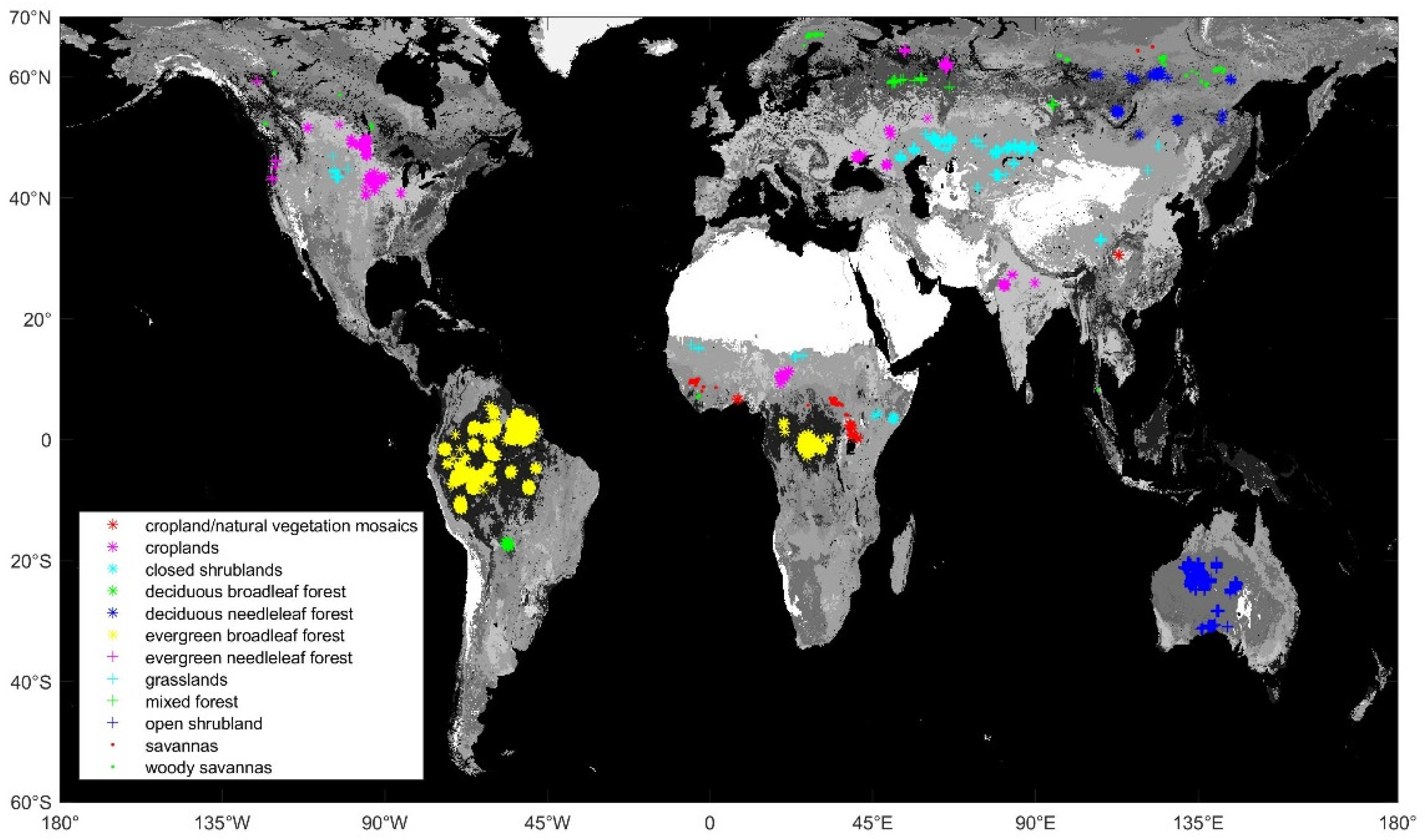
2.1. Passive Microwave Radiometers and Ancillary Data

Table 1. The datasets and adopted parameters used in this study.

Datasets	Parameters	Spatial Resolution	Temporal Resolution
L1C AMSR2	TBs	Varying with frequency	-
ERA5 hourly data on pressure levels	liquid water profile,water vapor profile, and atmosphere temperature profile	0.25 degrees	1 h
ERA5 hourly data on single level	SKT, surface pressure (SP), total column cloud liquid water content, snow depth and volume of water in soil layer of 0–7 cm	0.25 degrees	1 h
MCD12C1	global land cover types	0.05 degrees	-
MOD13C1	NDVI	0.05 degrees	16 days

presents the datasets and adopted parameters used in the study, as well as their temporal resolution and spatial resolution. The Advanced Microwave Scanning Radiometer-2 (AMSR2), onboard the Global Change Observation Mission 1st Water (GCOM-W1 or “SHIZUKU”) satellite, is a conical scanning passive microwave radiometer that operates at 6.925, 7.3, 10.65, 18.7, 23.8, 36.5 and 89 GHz with vertical (V) and horizontal (H) polarizations. Its incidence angle is about 55 degrees, and its ground resolution varies with the frequency: from 35 km × 62 km at 6.925 GHz to 3 km × 5 km at 89 GHz [43]. In this paper, the nearly 3-year Global Precipitation Measurement (GPM) Level 1C (L1C) (https://disc.gsfc.nasa.gov/datasets?keywords=1C&page=1&project=GPM,TRMM accessed on 19 July 2021) AMSR2 data [44] are adopted, which recalibrate the AMSR2 Level 1B data using GPM Microwave Imager (GMI) as the reference standard. The L1C AMSR2 data contain six frequencies from 10.65 GHz to 89 GHz. Since large temperature fluctuations during the day can lead to inaccurate temperature measurements [37,45], only the TBs from L1C AMSR2 that were observed during the night are used in this work.

Ancillary information required for atmospheric radiative transfer, including the liquid water profile, water vapor profile, and atmosphere temperature profile, is from ERA5 hourly data on pressure levels (https://cds.climate.copernicus.eu/cdsapp#!/dataset/reanalysis-era5-pressure-levels?tab=form accessed on 15 May 2022), i.e., the fifth generation European Centre for Medium-Range Weather Forecasts (ECMWF) reanalysis for the global climate and weather. The atmospheric data used here are hourly estimated, with a regular latitude-longitude grid of 0.25 degrees. In addition, land surface parameters, including the SKT, surface pressure (SP), total column cloud liquid water, snow depth, and volume of water in a soil layer of 0–7cm, are from ERA5 hourly data on single level (https://cds.climate.copernicus.eu/cdsapp#!/dataset/reanalysis-era5-single-levels?tab=overview accessed on 15 May 2022) with a spatial resolution of 0.25 degrees and a temporal resolution of 1 h.

The global MOD13C1 product (https://lpdaac.usgs.gov/products/mod13c1v061/ accessed on 15 January 2022) provides NDVI and is produced on 16-day intervals and at a spatial resolution of 0.05 degrees (~5.6 km at the equator). Land surface classification and coverage data employ the MODIS MCD12C1 Version 6 product (https://lpdaac.usgs.gov/products/mcd12c1v006/ accessed on 15 January 2022), which has a spatial resolution of 0.05 degrees. The land classification scheme adopts the IGBP global land cover classification system, which divides the earth surface into 16 types. However, only 12 vegetation types were selected for this research, as indicated in

Table 2. The screening criteria and results of pure pixels in MCD12C1 for 12 typical vegetation types.

Abbreviations	Land Cover Type	Screening Criteria	Count of Pure Pixels
ENF	evergreen needleleaf forests	$C_c$$> 95, C_7$$> 85, C_{wws}$$=0, C_{7\_wws}$< 5	183/N
EBF	evergreen broadleaf forests	$C_c$$=100, C_{21}$$> 98, C_{wws }$$=0, C_{21\_wws}$= 0	8901/N & S
DNF	deciduous needleleaf forests	$C_c$$> 80, C_3$$> 50, C_{wws}$$=0, C_{3\_wws}$< 5	71/N
DBF	deciduous broadleaf forests	$C_c$$> 95, C_{11}$$> 85, C_{wws}$$=0, C_{11\_wws}$< 5	125/S
MF	mixed forests	$C_c$$> 95, C_{11 }$$> 85, C_{wws}$$=0, C_{11\_wws}$< 5	128/N
CS	closed shrublands	$C_c$$> 95, C_7$$> 50, C_{wws}$$=0, C_{7\_wws}$< 5	23/N
OS	open shrublands	$C_c$$=100, C_{21}$$> 98, C_{wws}$$=0, C_{21\_wws}$= 0	3323/S
WS	woody savannas	$C_c$$> 90, C_{11}$$> 70, C_{wws }$$=0, C_{7\_wws }$< 5	746/N
-	savannas	$C_c$$> 95, C_{11}$$> 95, C_{wws}$$=0, C_{11\_wws}$< 1	606/N
-	grasslands	$C_c$$> 100, C_{21 }$$> 98, C_{wws}$$=0, C_{21\_wws}$= 0	1862/N
-	croplands	$C_c$$> 95, C_{11}$$> 95, C_{wws}$$=0, C_{11\_wws}$< 1	522/N
CNV	cropland/natural vegetation mosaics	$C_c$$> 80, C_{11}$$> 60, C_{wws}$$=0, C_{7\_wws}$< 5	48/N

.

Because of the lower spatial resolution of the microwave radiometer, many MCD12C1 data points can be present in the same AMSR2 footprint. Therefore, to have a single vegetation type within a footprint, as for a certain land type, the selection of its “pure pixel” in MCD12C1 should ensure higher coverage not only in the central pixel, but also in the surrounding pixels. On the other hand, if a certain land cover type has a small global distribution, the screening criterion should be lowered appropriately to obtain more samples. Since the microwave emissivity of water is much lower than that of land without water cover, pixels with high water and wetland coverage should be removed. In addition, to avoid the shielding effect of snow on the canopy, pixels with snow should also be excluded. As the seasons in the northern (N) and southern (S) hemispheres are opposite, samples from the same hemisphere are preferentially selected for each type. Evergreen broadleaf forests (EBF) are located near the equator, where seasonality is not apparent, so the pure pixels of this vegetation type are from both the S and N hemispheres.

Table 2 shows the abbreviations of the vegetation types, the screening criteria for the pure pixels, and the number of pure pixels in the N or S hemisphere for the 12 vegetated land types. Here, the letter $C_c$ represents the coverage in a central MCD12C1 pixel, $C_n$ is the coverage in surrounding n × n pixels, $C_{wws}$ is the water, wetland, and snow coverage in a central pixel, and $C_{n-wws}$ is the water, wetland and snow coverage in surrounding n × n pixels. Figure 1 shows the global distribution of pure pixels for the 12 vegetation types. EBF is concentrated in the Congo rainforest of Africa and the Amazon rainforest of South America. DBF is clustered in central South America and south of the Amazon rainforest. MF and DNF are located in the high latitudes of Europe and Asia, at about 60°N. CS is concentrated in eastern Africa, near the equator. OS is widely distributed in Australia. The other types are scattered across the continents. Croplands and grasslands are found in North America, Asia, Europe, and central Africa. CNV is mainly distributed in central Africa, and a few samples are present in the Sichuan basin of China. ENF is located in the eastern mountains and north of North America and northern Europe. Samples of savannas and WS are located across a wide latitude span, occurring at both low latitudes (central Africa) and high latitudes (North America and northern Europe and Asia). Moreover, two less obvious samples of WS are located in Malaysia.

To explore the relationship between instantaneous MLSE and land surface properties, the TBs were not averaged over time and space. The AMSR2 data falling on an MCD12C1 pixel were regarded as the TBs of that pixel. The matching of the AMSR2 and ERA5 data followed the rule of nearest proximity in time and space. Additionally, the NDVI data were first resampled to a spatial resolution of 0.25 degrees, and then spatially and temporally matched with AMSR2 data following the nearest neighbor rule.

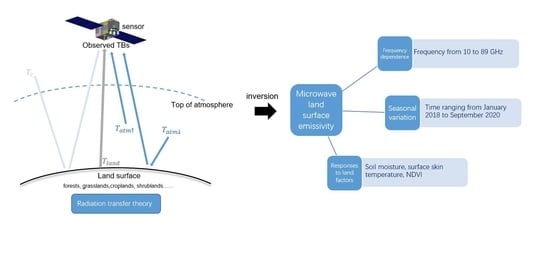
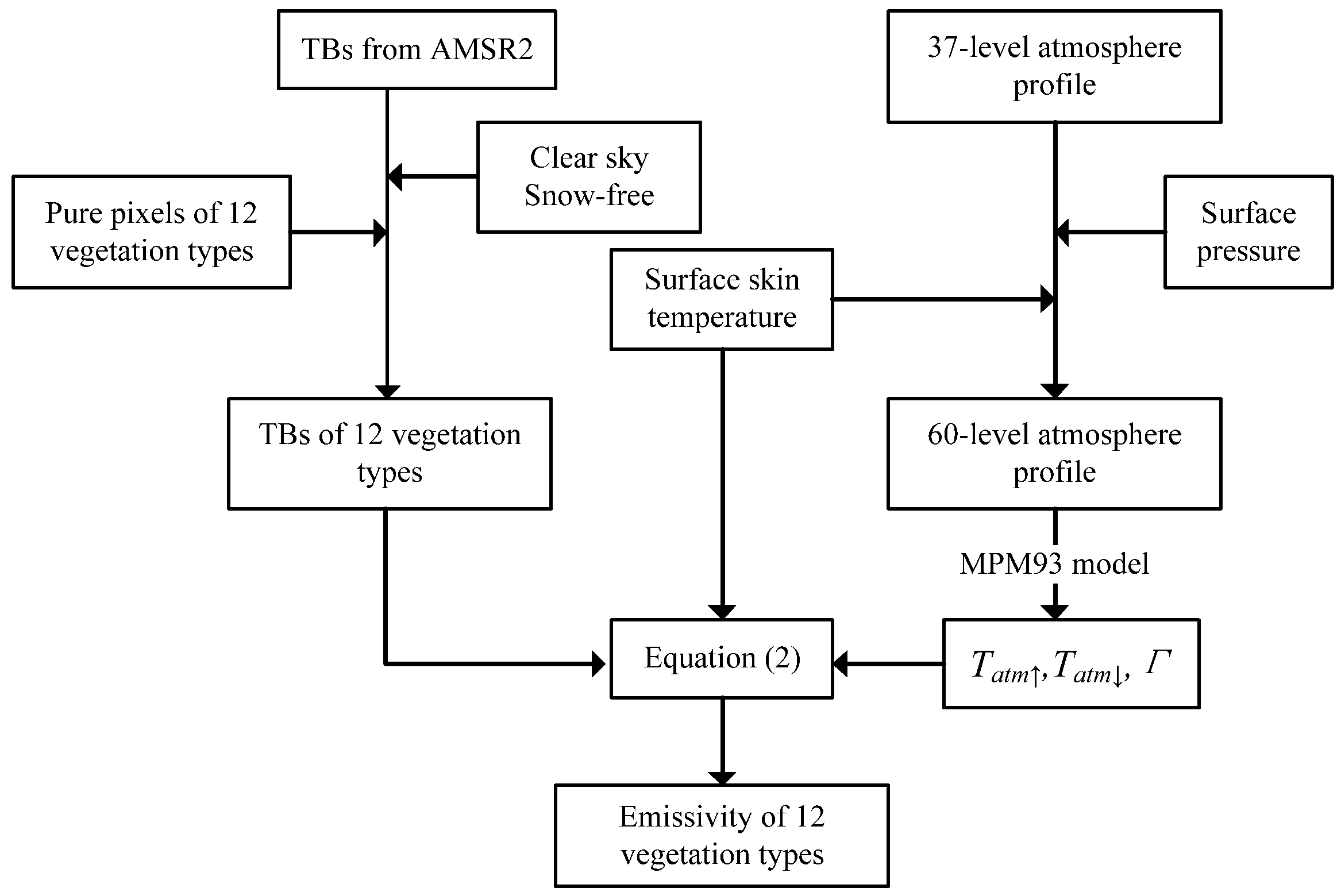
2.2. Instantaneous MLSE Retrieval

The retrieval is mainly based on radiative transfer theory. For the observation angle of 55°, the error introduced by treating the ground as a smooth surface can be negligible, especially in the window channels [21,23], so here it is used to simplify the radiative transfer. Assuming a plane parallel atmosphere with no scattering, the integrated radiative transfer equation in Rayleigh–Jeans approximation can be written as Equation (1) at given frequency f and polarization p [17]. From Equation (1), the signals received by the sensors consist of four components. The first and second terms are the upwelling radiations from the land surface and atmosphere. The third term describes the atmospheric downwelling radiation that is reflected by the land surface and received by the receiver. The fourth term represents the cosmic downwelling radiation that travels through the atmosphere to the surface and that is then reflected by the earth’s surface before re-penetrating the atmosphere, eventually entering the receiver.

$$\begin{array}{l}T{b}_{(f,p)}=e_{(f,p)}\cdot Ts\cdot \Gamma +T_{atm\uparrow }+T_{atm\downarrow }\left(1-e_{(f,p)}\right)\cdot \Gamma \\ +Tc\left(1-e_{(f,p)}\right)\cdot {\Gamma }^2\end{array}$$

(1)

The emissivity can be derived as

$$e_{\left(f,p\right)}=\frac{T{b}_{\left(f,p\right)}-T_{atm\uparrow }-Tc\cdot {\Gamma }^2}{Ts\cdot \Gamma -T_{atm\downarrow }\cdot \Gamma -Tc\cdot {\Gamma }^2}.$$

(2)

where $T{b}_{\left(f,p\right)}$ and $e_{\left(f,p\right)}$ are the TBs and emissivity at frequency f and polarization p; Ts is the surface skin temperature; $T_{atm\uparrow }={{\displaystyle \int }}_0^{H}T\left(z\right)\left[\alpha \left(z\right)/\mu \right]e^{-\tau \left(z,H\right)/\mu }dz$ is the atmospheric upwelling radiation; $T_{atm\downarrow }={{\displaystyle \int }}_H^{0}T\left(z\right)\left[\alpha \left(z\right)/\mu \right]e^{-\tau \left(z,0\right)/\mu }dz$ is the atmospheric downwelling radiation; $\Gamma =e^{-\tau \left(0,H\right)/\mu }$ is the transmittivity of the atmosphere; α(z) and T(z) are the atmosphere absorption and temperature at altitude z; $\mathsf{\tau }\left(z_1,z_2\right)={{\displaystyle \int }}_{z_1}^{z_2}\alpha \left(z\right)dz$ represents the atmosphere extinction from $z_1$ to $z_2$; μ is the cosine of the incidence angle on the surface; H is the orbiter height; and Tc is cosmic background TBs, 2.73 K.

Figure 2 shows the flow of instantaneous MLSE retrieval under cloud-free and snow-free conditions. In this work, it is assumed that total column cloud liquid water content less than 0.02 is for the clear sky retrievals [43]. The TBs with snow cover are removed using the indicator from the ERA5 data. After removing unwanted data, the TBs of the 12 vegetation types are selected according to the locations of their pure pixels.

In the theory of atmospheric radiative transfer, the calculation of atmospheric absorption is a core issue. The atmospheric profiles used here include liquid water (LW) profile, water vapor (WV) profile, and atmosphere temperature profile, and the ERA5 data divide the profiles vertically into 37 layers according to the pressure from the top of atmosphere to the land surface, with values ranging from 1 to 1000 hPa. However, the land surface pressure is not usually under ideal conditions, so it is necessary to adjust the profile levels according to the parameter SP. If SP is greater than 1000, SP and SKT are seen as the 38th-level pressure and temperature, and the corresponding LW and WV values are set to 0. Otherwise, the LW, WV, and temperature near the ground need to be recalculated by interpolation according to the position of SP in the 37-level pressure. After correcting the layers, the profiles are interpolated into 60 levels and the new profiles are used to calculate atmospheric absorption with the MPM93 model. $T_{atm\uparrow },$ $T_{atm\downarrow }$, and Γ can be obtained using the integral formula mentioned above, and finally emissivity can be easily determined with Equation (2).

3. Results

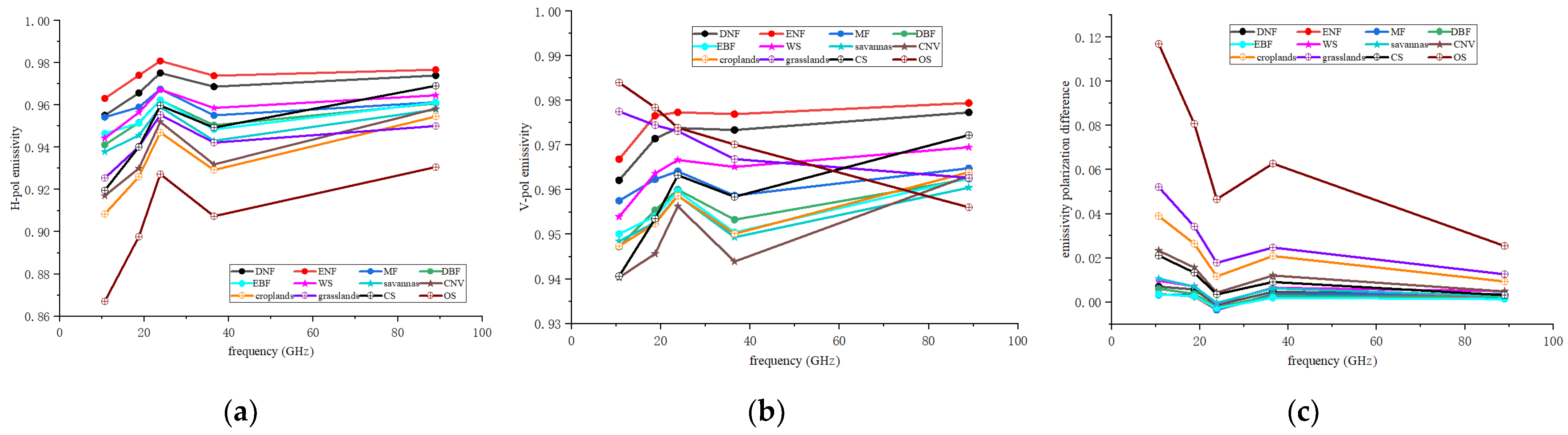
3.1. MLSE Spectral Features from 10.65 to 89 GHz

In summer, vegetation is in its prime growth period, and at this time, its emissivity is relatively stable and can be used as the characteristic emissivity. Therefore, the emissivity in summer (June–August in the North hemisphere and December–February in the South hemisphere) from 2018 to 2020 was used to analyze the spectral features of different vegetation types. For the 12 vegetation types, Figure 3 shows the mean emissivity of the H-pol, V-pol, and polarization differences (V-pol minus H-pol) as a function of frequency from 10.65 to 89 GHz.

In Figure 3a, the emissivity at H-pol is positively correlated with vegetation biomass. The two types of coniferous forests show the largest emissivity. WS, MF, DBF, EBF, and SAV have relatively higher biomass and emissivity values, and their emissivity values are comparable and indistinguishable. It is worth noting that the emissivity of CS, OS, grasslands, CNV, and croplands is relatively small at 10.65 GHz, but it increases rapidly with frequency, and the emissivity of CS even exceeds that of broadleaf forest at 89 GHz. Therefore, the difference of vegetation microwave radiation characteristics decreases with frequency, and the low-frequency emissivity is more helpful in distinguishing vegetation biomass. Remarkably, OS exhibits the lowest emissivity at all frequencies due to relatively sparse plants with coverage of 10–60%. In general, the H-pol emissivity increases with frequency. The emissivity peak at 23.8 GHz is widely present in all vegetation types, which may be related to the incomplete removal of water vapor absorption from the atmosphere. The emissivity of 18.7 GHz in MF and EBF is slightly less than that of 36.5 GHz, which can also be found in the results of LiRui et al. [1], Min et al. [46], and Li et al. [10]. Li et al. [10] attributed it to scattering depression from the vegetation elements, such as leaves, stems, and branches.

Compared to Figure 3a, the V-pol emissivity displays a smaller range of variations and a more complicated picture that the response of V-pol emissivity to vegetation biomass or density is different from that of H-pol. This issue may be explained by the different response of the roughness effect to the two polarizations [47]. In addition, there is an apparent anomaly in grasslands and OS that their emissivity decreases with increasing frequency. We speculate that this phenomenon may be caused by volume scattering. According to previous research [48,49], volume scattering generally occurs in bare soil and snow, where particles strongly scatter the upwelling radiation, leading to decreased emissivity. Moreover, the scattering effect increases with frequency, resulting in a negative correlation between emissivity and frequency. Here, the relatively sparse and low plants in grasslands and OS allow the signals from the soil to be detected, thus leading to this abnormal phenomenon. Besides, unusually high emissivity at low frequencies is discovered in grasslands and OS, and the most likely explanation for this is inconsistencies between the effective temperature and SKT in arid and semi-arid areas [22,26,33]. Under the joint action of many factors, it is difficult to interpret the spectral behaviors of V-pol emissivity. Further investigations need to be carried out to understand the complex problem.

From Figure 3a,b, the emissivity of needleleaf forests is apparently greater than that of broadleaf forests, regardless of the frequency and polarization. Wegmuller et al. [50] also observed this phenomenon. Matzler [51] pointed out that leaf orientation can make a difference in the emissivity of vegetation, that is, horizontal leaves usually have a lower emissivity than vertical leaves. Moreover, the water content in needleleaf is usually lower than that in broadleaf, which may be another possible factor explaining this issue.

According to Figure 3c, the polarization difference of emissivity is negatively correlated with vegetation biomass, and the densely vegetated types (several forest types) exhibit negligible polarization differences. In general, leaves in the canopy are randomly oriented and radiation is almost independent of polarization. With the increase in vegetation density, H-pol radiation strengthens, while V-pol radiation weakens, leading to a decrease in polarization difference [19]. Additionally, the emissivity polarization difference generally decreases with increasing frequency, because the relative roughness of the vegetation surface increases with the frequency and indirectly contributes to a smaller polarization difference. Over the dense vegetation types, the polarization differences at 23.8 GHz are slightly negative, which is unexpected, and Prigent et al. [18] suspected that it is caused by a calibration error.

Above all, the emissivity of vegetation shows a high value that is generally greater than 0.9 between 10.65 and 89 GHz for non-sparse vegetation areas. As the frequency increases, the emissivity of different vegetation types gradually converges. The compact values make it difficult to accurately distinguish different vegetation types using emissivity alone. However, dense forests and sparse vegetation can be clearly recognized at 10.65 GHz according to their polarization difference.

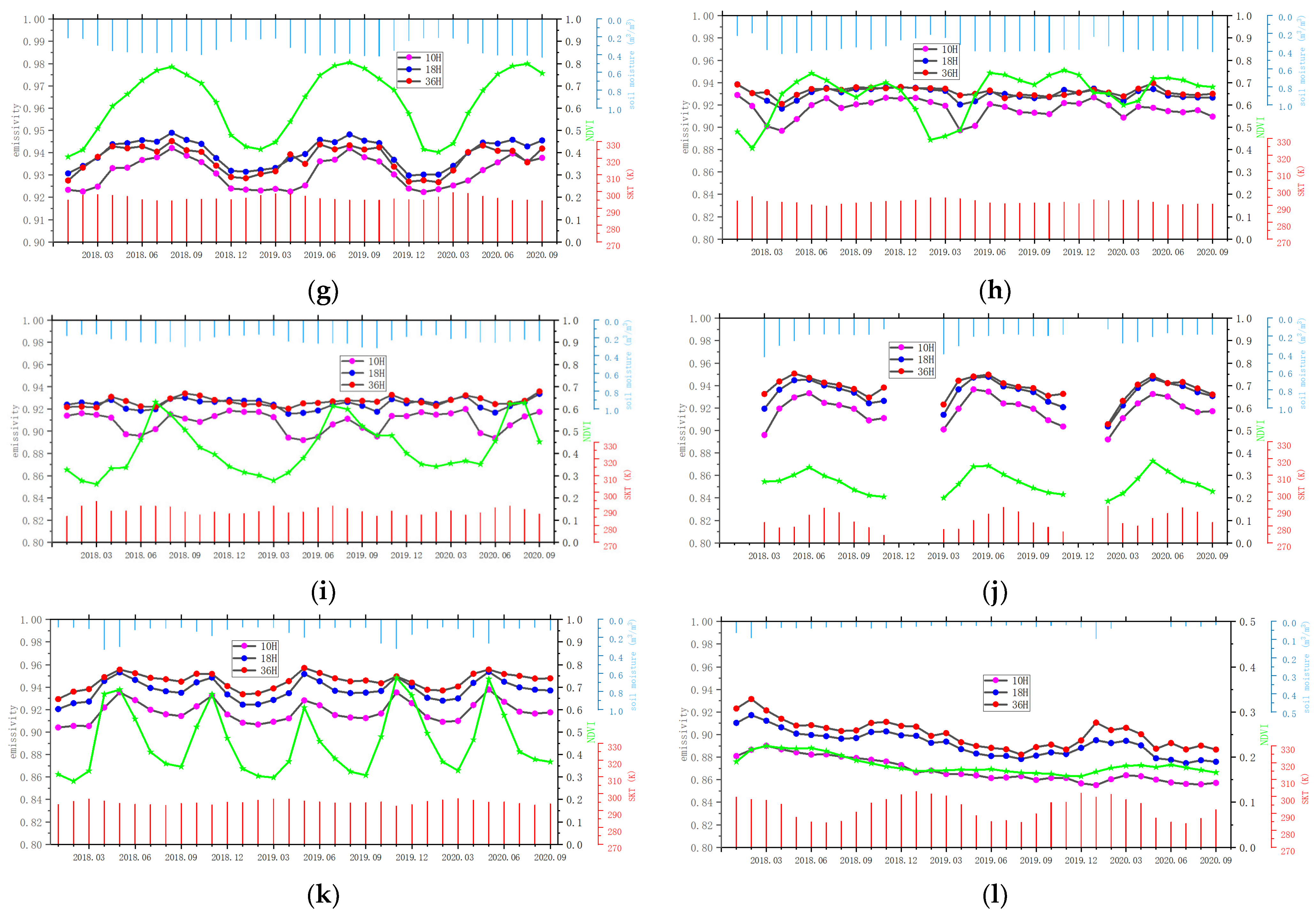
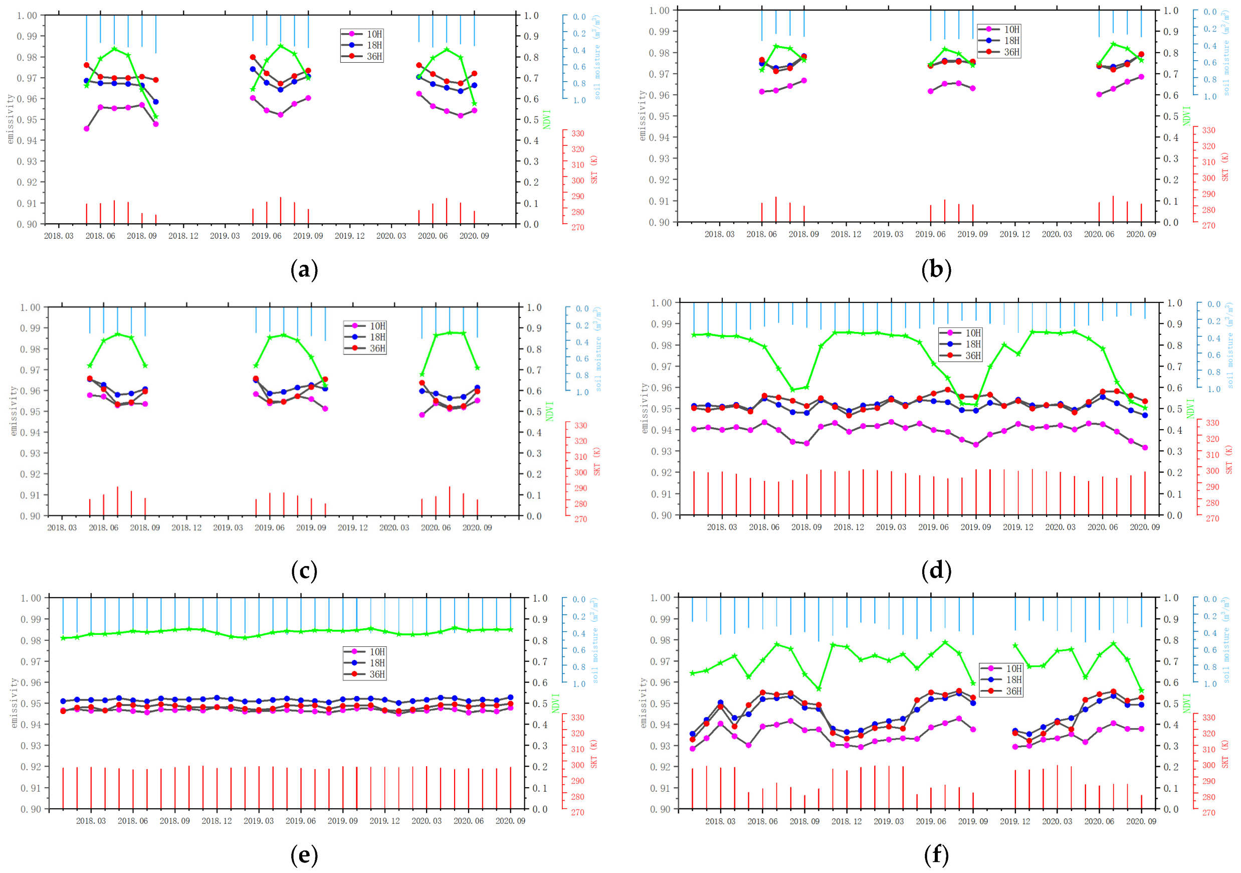
3.2. Temporal Variations of MLSE

At given vegetation types, temporal variations of MLSE can reflect seasonal changes in vegetation characteristics, such as biomass and water content. Figure 4 shows the time series of the monthly mean emissivity at three window frequencies (10.65, 18.7, and 36.5) in H-pol (Hereinafter referred to as 10H, 18H and 36H) for 12 vegetated areas, with time ranging from January 2018 to September 2020. Overlapped are associated time series of NDVI, SKT, and SMC. Since snow-covered data points have been removed, the figures of ENF, DNF, MF, WS, and grasslands show incomplete annual cycles.

In Figure 4a–c, temporal variations of DNF, ENF, and MF are limited in the late spring, summer, and early fall months. The amplitudes of the curves in the three figures are weak, with the range (the difference between the maximum value and the minimum value) less than 0.02. The variations of NDVI have good consistency with the temperature, rising first and then declining, and the peak value generally occurs in July. Unexpectedly, the seasonal variations of emissivity are negatively correlated with that of NDVI and SKT in some cases, and it seems that the higher the frequency, the more pronounced this phenomenon is. This puzzling problem also appeared in the results of Li et al. [1], for reasons that remain unknown.

In Figure 4a, the higher soil moisture in May 2018 had a different influence on the 10H, 18H, and 36H emissivity. On the 10H curve, the SMC had a great effect, leading to a sudden decrease in emissivity. For the 18H curve, the SMC showed a moderate impact, neutralizing the upward trend of emissivity. As for the 36H curve, the SMC had a weakened effect, and the emissivity remained at a higher value. Moreover, in October 2018, NDVI declined rapidly, resulting in a significant decrease in the 10H emissivity, a moderate decrease in the 18H emissivity, and a slight decrease in the 36H emissivity.

A similar phenomenon also appears in October 2019, as shown in Figure 4c. The above analysis indicates that with the increase of frequency, the sensitivity of microwave to vegetation and soil decreases, and the 36H emissivity is less sensitive to soil moisture in forest areas.

In Figure 4d, emissivity shows clear seasonal variation and a mild amplitude. Along the 10H emissivity curve, there are small valleys in August and September every year, which is consistent with NDVI. The 18H emissivity has a similar variation pattern to the 10H emissivity, but with a smaller amplitude. The curve of the 36H emissivity has a consistent inflection point with that of the 18H emissivity, but with a larger rise and smaller decline. As for EBF, in Figure 4e, the amplitude of the seasonal variation is the smallest among all the 12 types, with a range less than 0.005. EBF is located in tropical rainforest regions, which are warm and rainy all year round, and this vegetation type does not experience an obvious annual cycle of growth and senescence. Over the years, the emissivity at the three frequencies remained extremely stable.

In Figure 4f, since the samples of WS have a large latitude range from 0 to 70°N, the emissivity curves display two characteristics with time: vegetation in high-latitude region dominates from May to October, while vegetation in the equatorial area dominates in other months when the high-latitude areas are covered by snow. Every year from May to October, the variation trend of the 10H emissivity is similar to that of NDVI and SKT, and the variations in 18H and 36H occur significantly earlier, one month before. Moreover, NDVI declined rapidly from July 2019 to September 2019, while emissivity remains at a high level and shows a slight downward trend in September. The above statements reveal that temporal variations in NDVI and emissivity at different frequencies do not always change in sync, perhaps due to differences in their sensitivity to different vegetation features. Additionally, although the NDVI is comparable in winter and summer, the emissivity in winter is significantly lower than that in summer. This can be attributed to the other possible effects that contribute to emissivity.

As for savannas, as shown in Figure 4g, the temporal variations in emissivity are highly season-related, consistent with NDVI and negatively correlated with temperature. The three curves have moderate amplitudes, and the range is close to 0.02. The emissivity peaks occur every summer and are highly consistent with soil moisture, indicating that water in the soil is an important factor affecting the growth of savannas.

In Figure 4h, the 10H emissivity curve displays clear fluctuations, and there is an obvious time deviation in the temporal variation between emissivity and NDVI. The first valley value of emissivity occurs in April 2018 and lags significantly behind that of NDVI by two months. In addition, NDVI showed a trough from February to April 2019, while emissivity showed the corresponding trough two months later. The time deviation indicates that the changes in vegetation elements that are related to microwave radiation, such as water content, are not always synchronized with the variations in chlorophyll represented by NDVI. The variation intensity of 10H is greater than that of 18H and 36H, proving once again that the higher the frequency, the less sensitive it is to the land surface state.

Cropland is a complex vegetation type with strong variability and inhomogeneity. Different climates can lead to different crops with diverse plant heights, leaf shapes, planting densities, and soil conditions. From Figure 1, the pure pixels of croplands are located across several continents, with most of the samples in temperate climates and a small number in tropical climates. Summer is the peak period for crop growth and generally shows higher NDVI and emissivity. However, for croplands in tropical areas, they will show a lower emissivity because of their relatively higher soil moisture. As shown in Figure 4i, the 10H curve has several distinct troughs associated with tropical crops that occur from May to July of 2018, from April to June of 2019, and from May to July of 2020. The SMC does not show higher values during the corresponding periods because fewer data from tropical areas were lost during the statistical process. In addition, there are troughs in October 2018 and 2019, which are due to this time representing the harvest period in temperate croplands. In winter, NDVI is low, but 10H emissivity is at a high level. This inconsistency is also observed in Figure 4f and has been explained previously. Moreover, the amplitudes of 18H and 36H are significantly less than that of 10H because of the weaker sensitivity to soil moisture. In any case, it is surprising that the 10H emissivity can reveal more details regarding the seasonal variations in vegetation than NDVI, especially in terms of soil moisture information.

In Figure 4j, the NDVI of grasslands is always at a low level but has clear seasonal variation characteristics. The variation of emissivity is highly consistent with that of NDVI, but with a greater amplitude. An interesting phenomenon can be observed: emissivity and NDVI usually peak in May or June rather than in July, which is when temperatures are the highest. The most likely reason for this is the effect of soil moisture on vegetation growth. In spring, the higher soil moisture encourages grass growth, leading to a rapid increase in emissivity. In summer, the arid climate inhibits growth, resulting in a slow decline in emissivity. In addition, it should be noted that the effect of soil moisture on grass growth demonstrates a certain time lag here.

In Figure 4k, the three emissivity curves show apparent seasonal variation with a large amplitude. Since samples of CS are located in the region between the northern loop and the equator, where the sun shines directly twice a year, there are five peaks in the NDVI and emissivity curves. Similar to the situation observed for savannas, the peaks are highly correlated with soil moisture, indicating that the growth of CS is strongly dependent on the water in the soil.

Although both are shrublands, the situation with OS is completely different from that of CS. From Figure 4l, the emissivity and NDVI of OS are relatively low all the time with little seasonal variation. According to the changes in NDVI over the past three years, the vegetation density or growing status of OS is on a declining trend, leading to reduced emissivity. In January and February of 2018, the relatively high soil moisture resulted in distinct peaks in the three emissivity curves, and the higher the frequency, the more pronounced the peak. Moreover, in January 2020, the higher soil moisture corresponds to high emissivity at 36H and 18H, but low emissivity at 10H. This phenomenon proves that the effect of soil moisture on vegetation emissivity is very complex. In general, microwave radiation at 18 and 36 GHz is mainly from the vegetation canopy, while that of 10 GHz is from both the vegetation and soil. With the increase of soil moisture, vegetation grows rapidly, leading to the enhancement of two high-frequency radiation. However, 10 GHz radiation may increase or decrease, depending on the complex physical interactions between the vegetation and soil.

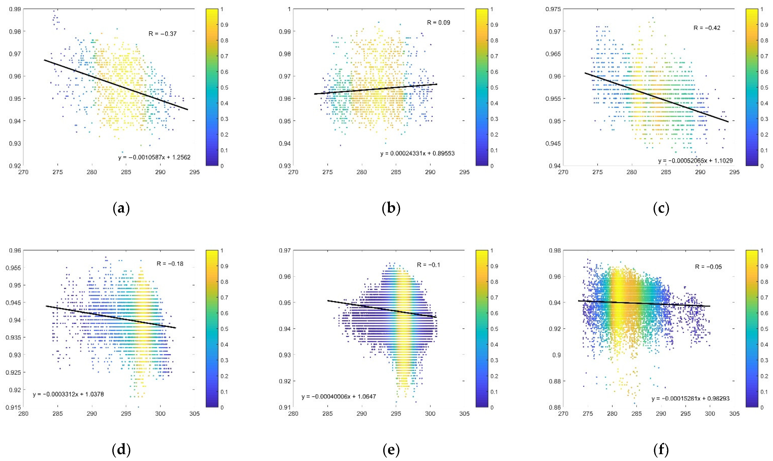
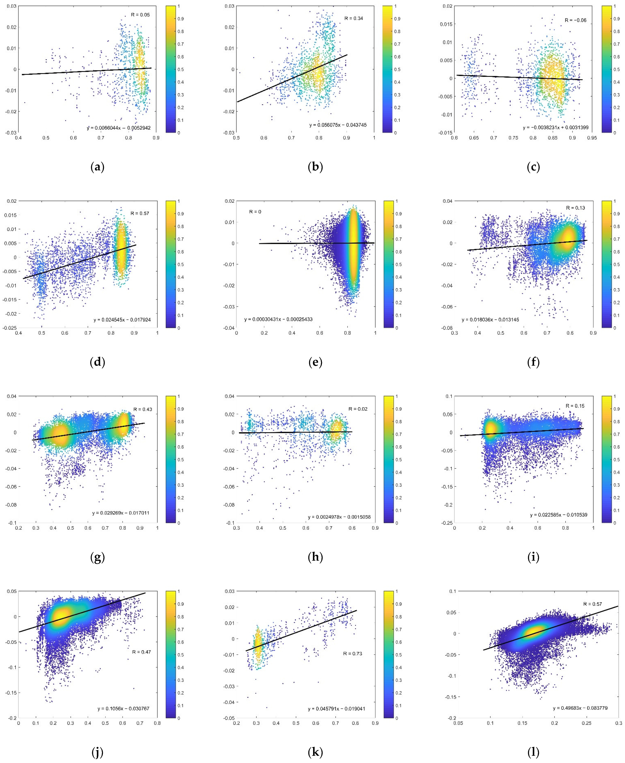
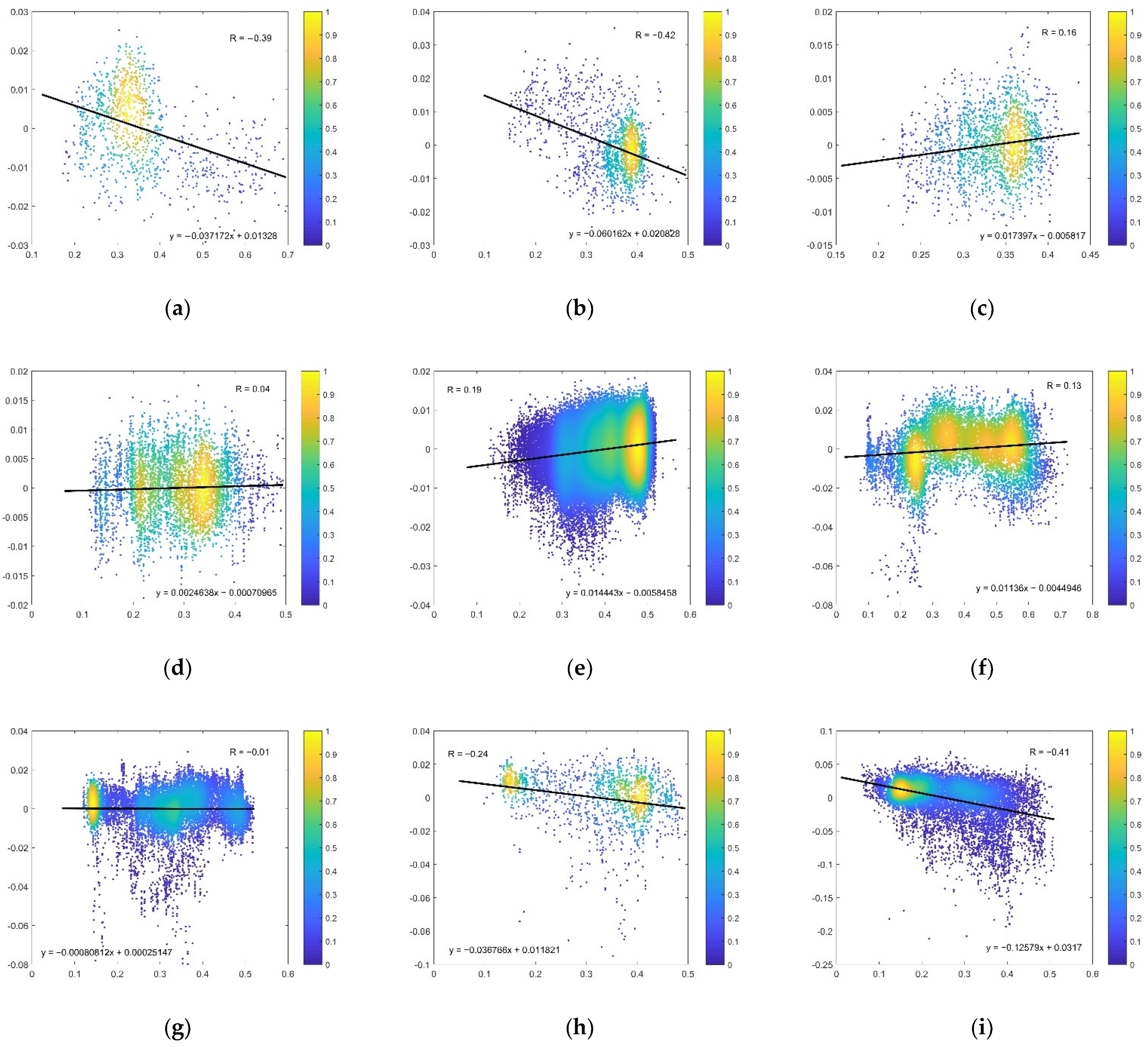
3.3. Responses of 10H Emissivity to SKT, NDVI and SMC

As low-frequency radiation is less affected by atmospheric composition, and H-pol emissivity is more sensitive to land surface information, the 10H channel was selected here to explore the relationship between emissivity and land surface parameters. In terms of availability, the three factors, including NDVI, SMC, and SKT, were chosen as candidates for the correlation analysis.

During a seasonal cycle, SKT is a variable that experiences large variation, followed by NDVI, and SMC shows the smallest change. In statistical processes, large influencing factors can mask the role of small influencing factors. For example, if temperature has a great effect on emissivity, and SMC has a weaker impact on emissivity, it is difficult to determine the true correlation between emissivity and SMC without removing the influence of temperature. To avoid the above problem, we propose a step-by-step method for stripping the impact factors and introduce two intermediate variables, Delta1 and Delta2, to the correlation analysis. Equations (3) and (4) show the calculation of Delta1 and Delta2. In these equations, Ts is the surface skin temperature; $p_1$ and $p_2$ are the fitting coefficients of SKT for the linear equation that is the best fit (in a least-squares sense) for the 10H emissivity; $p_3$ and $p_4$ are the linear fitting coefficients of NDVI for the equation that is the best fit for the Delta1. The values of $p_1$,$p_2$,$p_3$, and $p_4$ are presented in Appendix A. Using this method, the influence of SKT can be stripped in rough when discussing the impact of NDVI on emissivity, and the contributions of SKT and NDVI can be roughly removed when discussing the influence of SMC on emissivity.

$$\mathrm{Delta}1=e_{\left(10.65,H\right)}-\left(p_1\times Ts+p_2\right)$$

(3)

$$\mathrm{Delta}2=\mathrm{Delta}1-\left(p_3\times NDVI+p_4\right)$$

(4)

According to the instantaneous MLSE retrieved in 2019, Figure 5, Figure 6 and Figure 7 show the density scatter diagrams for the 12 vegetation types between SKT and the 10H emissivity, NDVI and Delta1, and SMC and Delta2. R represents the correlation coefficient, and the black line is the regression line that fits the scatter points.

In Figure 5, the emissivity of most vegetation types shows a weak positive or negative correlation with SKT, and the larger absolute values appear in DNF, MF, savannas, and CS. In general, as the surface temperature increases, the radiation energy of both the blackbody and land surface increase, but the temperature increase of the blackbody is greater than that of the land surface, leading to a smaller ratio, that is, emissivity [52]. However, the effect of SKT on emissivity should be relatively small, and the large correlations in the four types should be attributed to other possible reasons. From Figure 1 and Figure 4g, the samples of savannas mostly located near the equator can be seen to experience different periods of rain and heat. A likely explanation for this is that emissivity is mainly affected by NDVI, the variation of which is opposite to that of temperature, which indirectly leads to a negative correlation between emissivity and temperature. The same reason can also apply to CS, while the possible reason for DNF and MF requires further investigation. On the other hand, rising temperatures encourage vegetation to grow and counteract its negative effects to some extent, so it is also reasonable for the weak positive correlations in figures of ENF and croplands.

As shown in Figure 6, the correlation between Dalta1 and NDVI varies with different vegetation types. In the figures of grasslands, CS and OS, Delta1 is highly dependent on NDVI, which indicates that the emissivity of low-biomass vegetation is mainly determined by plant growth. Moreover, an interesting phenomenon can be seen in Figure 6j, in which Delta1 first increases with NDVI when NDVI is lower, and then Delta1 increases slowly or tends to be saturated with the further increase of NDVI. This indicates that the positive role of NDVI can weaken with the increase of NDVI. For DBF and savannas, which show a clear annual cycle of growth and senescence, the response of Delta1 to NDVI is also strongly positive, with correlation coefficients of 0.57 and 0.43. ENF exhibits a moderate correlation with R of 0.34, and WS and croplands show relatively low correlation, with values of 0.13 and 0.15. For DNF, MF, and EBF, the dense vegetation types with less seasonal variation, the role of NDVI can be negligible. In addition, due to the significant asynchrony of the temporal variations between emissivity and NDVI, the R of CNV also shows a relatively low value.

As for the response of emissivity to SMC, there is a more complicated case. On the one hand, soil moisture promotes vegetation growth, which in turn increases emissivity. On the other hand, due to the large dielectric constant of water, increasing soil moisture will reduce emissivity if the soil can be detected. Therefore, whether the correlation between emissivity and SMC is positive or negative depends on the complex interaction between vegetation and soil. In Figure 7a,b, the values of Delta2 show a strong negative correlation, while the other forest types exhibit a weak positive correlation. The possible reason for this is that needle leaves, which are not dense enough, have gaps that allow soil information to be detected. On the contrary, broadleaves with large leaf area can better conceal ground signals and thus only show positive effects of soil moisture. In Figure 7i, R has a larger negative value of −0.41, indicating that SMC has a dominant negative effect on croplands, which is also reflected in the lower emissivity of tropical croplands, which had a higher SMC in the previous section.

In Figure 4d,g,j,k, SMC plays a positive role in the growth of DBF, savannas, grasslands, and CS, whereas the correlation coefficients are small positive or negative values in Figure 7d,g,j,k. For the four types, SMC and NDVI experience coupling in which NDVI increases with SMC. In the process of removing the dependence of NDVI, the positive effect of SMC is also weakened, and only the slightly positive or negative effect is retained. As for MF, EBF, and WS, SMC has a relatively weak positive effect on their emissivity, with correlation coefficients of 0.16, 0.19, and 0.13. In addition, an interesting phenomenon can be observed in Figure 7f: SMC plays a positive role on Delta2 when its value is less than 0.3, and SMC shows a negative effect as it further increases. This phenomenon reveals that the positive effect of SMC is dominant under drought conditions because of the dependence of vegetation growth on soil moisture, and the negative effects were more common under humid conditions.

Above all, each vegetation type has one or two highly correlated influence factors, except for EBF, CNV, and WS. EBF has almost no fluctuations in emissivity and the three factors, leading to a poor correlation. From Figure 4h, the variations in emissivity for CNV are obviously out of sync with the changes in the factors, resulting in a low correlation. The same reason can partly explain the low correlation of WS. Moreover, according to Figure 1 and Figure 4f, the emissivity of WS displays two characteristics, and the relatively stable emissivity at low latitudes can reduce the overall correlation. Besides, R can only represent the degree of linear correlation, and it cannot show the nonlinear part between Delta2 and SMC.

4. Discussion

To understand the microwave radiation characteristics of different vegetation types, the observed TBs were used to retrieve the emissivity for the typical vegetated land types. Although the retrieval was conducted under clear sky, inaccuracies in the atmospheric profile data and the incomplete removal of cloud can introduce errors. According to the MLSE spectral behaviors in this paper, the retrieved values show good performances in the atmospheric window bands. Nevertheless, there is still atmospheric contamination at 23.8 GHz, i.e., the water vapor absorption channel. This has also been discovered in previous results [23,32,41], and efforts to deal with the complex physical problem have been made.

The discrepancy between the effective temperature and the surface skin temperature is another thorny problem. Microwave has relatively strong penetration ability and can obtain information about the vertical structure of vegetation, woody parts, and soil. This feature can extend our understanding of the Earth’s surface, but it also introduces difficulties in MLSE retrieval. In areas with sparse vegetation, the microwave signals are from vegetation and the soil within a certain depth. Therefore, the corresponding temperature used in Equation (2) should theoretically be the comprehensive contribution within the penetration depth, i.e., the effective temperature.

In the absence of direct effective temperature information at relatively large spatial scales, some scholars have attempted to deal with effective temperature using physical models. Prigent et al. [26] calculated the temperature at different depths in desert areas with a one-dimensional, time-dependent heat conduction model. Later, Moncet et al. [21] improved on Prigent’s model and applied it to semi-arid areas. Norouzi et al. [22] built a lookup table of effective temperature using Prigent’s model to reduce globally the day-night discrepancies of MLSE. Prakash et al. [20] proposed a statistical correction factor for arid regions that used the monthly mean TB and mean daily skin temperature. However, the land surface is very complex, especially in vegetation-covered areas. The heat conduction model can make sense over bare land but may not work well in vegetated areas. Moreover, the effective temperature in the lookup table can hardly explain the dynamic variability of the land surface. In this work, since the calculation of instantaneous emissivity has high requirements for the temporal resolution of the input data, the SKT from ERA5 was used. Although there are some errors in the low-frequency emissivity of grasslands and OS, it is acceptable for the other vegetation types. In future work, how to deal with this problem will be one of the main goals.

In Section 3.2, it was shown that the variation of emissivity can be ahead or behind that of NDVI in the annual cycle of the seasons, indicating that microwaves and optics are sensitive to the different vegetation elements that change asynchronously. NDVI is calculated by the reflectivity values of visible and near infrared bands, which are influenced by the chlorophyll content in leaves. While the microwave bands are mainly determined by the dielectric constant, they are mostly sensitive to the water content of the vegetation. The inconsistency between emissivity and NDVI changes reveals that the time and intensity of changes in chlorophyll may be different from the changes in the vegetation water content at the turn of the seasons. Moreover, the time curve of cropland emissivity shows two distinct characteristics, one for temperate farmland and the other for tropical farmland. Cropland is almost the most complex type of vegetation and is strongly influenced by human activities. The characteristics of different crops vary greatly, so further subdivision of cropland into subtypes will help to improve our understanding of its emissivity.

The responses of the 10H emissivity to SKT, NDVI, and SMC is significantly complex. In general, with the rise of surface temperature, the increased energy of the black body is greater than that of the land surface, resulting in a slight decrease in emissivity. On the other hand, a higher SKT can promote vegetation growth, compensating for the negative response of emissivity to temperature. According to previous studies [11,38,53], NDVI usually has a positive effect on MLSE. However, the temporal variation of emissivity may occur before or after the temporal variation of NDVI, which may reduce the correlation significantly. As for SMC, one would expect a reduction in emissivity under high soil moisture according to previous arguments. However, soil moisture can promote vegetation growth, resulting in a higher emissivity. Therefore, both the positive and negative effects of SMC on vegetation emissivity are reasonable. In relatively arid regions, increased soil moisture caused by precipitation should have a negative effect on emissivity in the short term (within several hours or a day) but a positive effect in the long term [1]. Furthermore, as shown in Figure 7f, SMC can promote emissivity when it has a relatively low value. As SMC increases further, its negative effects can play a leading role. In addition, three factors cannot fully explain the change of MLSE, so there are some outliers in Figure 5, Figure 6 and Figure 7. Accordingly, other factors still need to be considered for further study.

In addition, there is a limitation in the step-by-step method that the dependency of the factor removed in the previous step can sometimes weaken the effect of the next factor because there are coupling effects between those factors. Moreover, correlation can only reflect the linear relationship between two variables, while it is difficult for this parameter to reflect the nonlinear relationship.

5. Conclusions

In summer, the emissivity of vegetation is high and increases with frequency. The H-pol emissivity has a larger dynamic range than the V-pol emissivity, indicating that H polarization has a stronger sensitivity to the land surface than V polarization. Moreover, H-pol emissivity is positively correlated to vegetation biomass or density, while the polarization difference is negatively correlated with vegetation biomass. An unusual phenomenon occurs in the V-pol emissivity of grasslands and OS that declines with increasing frequency, and the possible cause of it is the volume scattering effect.

The seasonal variations in the monthly mean emissivity at 10H, 18H, and 36H vary with vegetation type. The amplitude of emissivity variation in evergreen forests is significantly small, especially for EBF, with little change being observed over the years. DBF, DNF, MF, WS, and savannas show moderate amplitude of variation, with a range of less than 0.02. CNV, croplands, CS, and OS display relatively large seasonal fluctuations, and grasslands show the largest dynamic variation range of more than 0.04. For most vegetation types, the seasonal variation trends of emissivity are consistent with those of NDVI. As for WS, CNV, and croplands, the changes in NDVI and emissivity are asynchronous.

As for the responses of the 10H emissivity to SKT, NDVI, and SMC, the main results are as follows. For most vegetation types, SKT shows a relatively weak effect. However, for DNF, MF, savannas, and CS, SKT has a relatively strong negative correlation with emissivity, with the correlation coefficient R of −0.37, −0.42, −0.46, and −0.32. NDVI plays a positive role in MLSE for several vegetation types. For DBF, CS, grassland and OS, the emissivity is strongly driven by NDVI, with R values greater than 0.45. In grasslands, it is worth noting that the positive effect of NDVI can be weakened with the increase of NDVI. Savannas and ENF display a moderate positive correlation with NDVI, with R of 0.43 and 0.34. WS and CROP show a weak positive correlation with NDVI, and their correlation coefficients are 0.13 and 0.15. For DNF, MF and EBF, the dense vegetation types with less seasonal variation, the role of NDVI can be negligible. In addition, due to the significant asynchrony of the temporal variations between emissivity and NDVI, R also has a relatively small value in CNV. In this paper, the negative effect of SMC can be clearly seen in DNF, ENF, and croplands, which have R values of −0.39, −0.42, and −0.41. The values of R are also negative for savannas, grasslands, and CS, which clearly contradicts the results in Figure 4. This is because the positive role of SMC is weakened when the dependence of NDVI is removed, as described in Section 4.

The vegetated areas are significantly complex land covers, the microwave radiation of which has always been a challenging subject in remote sensing. Based on the idea that the same vegetation cover land has similar radiation characteristics, we selected pure pixels of 12 vegetated land types from the global scale, and then analyzed the responses of their emissivity to possible factors, respectively. The promising results obtained here can help build a land cover type-oriented emissivity model in future work. On the other hand, due to relatively stronger penetration ability, the results of microwave detection can provide a new perspective for vegetation monitoring from space and can supplement the results of optical remote sensing.

References

1. Li, R.; Hu, J.; Wu, S.; Zhang, P.; Letu, H.; Wang, Y.; Wang, X.; Fu, Y.; Zhou, R.; Sun, L. Spatiotemporal Variations of Microwave Land Surface Emissivity (MLSE) over China Derived from Four-Year Recalibrated Fengyun 3B MWRI Data. Adv. Atmos. Sci. 2022, 39, 1536–1560. [Google Scholar] [CrossRef]
2. Qiu, Y.; Guo, H.; Shi, J.; Lemmetyinen, J.; Shi, L. An emissivity-based land surface temperature retrieval algorithm. In Proceedings of the 2012 IEEE International Geoscience and Remote Sensing Symposium, Munich, Germany, 22–27 July 2012. [Google Scholar] [CrossRef]
3. Yin, C.L.; Meng, F.; Yu, Q.R. Calculation of land surface emissivity and retrieval of land surface temperature based on a spectral mixing model. Infrared Phys. Technol. 2020, 108, 103333. [Google Scholar] [CrossRef]
4. Zhao, T.; Shi, J.; Bindlish, R.; Jackson, T.; Cosh, M.; Jiang, L.; Zhang, Z.; Lan, H. Parametric exponentially correlated surface emission model for L-band passive microwave soil moisture retrieval. Phys. Chem. Earth Parts ABC 2015, 83, 65–74. [Google Scholar] [CrossRef]
5. Rodriguez-Fernandez, N.J.; Aires, F.; Richaume, P.; Kerr, Y.H.; Prigent, C.; Kolassa, J.; Drusch, M. Soil Moisture Retrieval Using Neural Networks: Application to SMOS. IEEE Trans. Geosci. Remote Sens. 2015, 53, 5991–6007. [Google Scholar] [CrossRef]
6. Wigneron, J.P.; Jackson, T.J.; O’Neill, P.; De Lannoy, G.; de Rosnay, P.; Walker, J.P.; Ferrazzoli, P.; Mironov, V.; Bircher, S.; Grant, J.P.; et al. Modelling the passive microwave signature from land surfaces: A review of recent results and application to the L-Band SMOS & SMAP soil moisture retrieval algorithms. Remote Sens. Environ. 2017, 192, 238–262. [Google Scholar] [CrossRef]
7. Li, Z.L.; Leng, P.; Zhou, C.; Chen, K.S.; Zhou, F.C.; Shang, G.F. Soil moisture retrieval from remote sensing measurements: Current knowledge and directions for the future. Earth-Sci. Rev. 2021, 218, 103673. [Google Scholar] [CrossRef]
8. Moradizadeh, M.; Srivastava, P.K. A new model for an improved AMSR2 satellite soil moisture retrieval over agricultural areas. Comput. Electron. Agric. 2021, 186, 106205. [Google Scholar] [CrossRef]
9. Zhang, S.; Weng, F.; Yao, W. A Multivariable Approach for Estimating Soil Moisture from Microwave Radiation Imager (MWRI). J. Meteorol. Res. 2020, 34, 732–747. [Google Scholar] [CrossRef]
10. Li, R.; Min, Q. Dynamic response of microwave land surface properties to precipitation in Amazon rainforest. Remote Sens. Environ. 2013, 133, 183–192. [Google Scholar] [CrossRef]
11. Li, R.; Wang, Y.; Hu, J.; Wang, Y.; Min, Q.; Bergeron, Y.; Valeria, O.; Gao, Z.; Liu, J.; Fu, Y. Spatiotemporal variations of satellite microwave emissivity difference vegetation index in China under clear and cloudy skies. Earth Space Sci. 2020, 7, e2020EA001145. [Google Scholar] [CrossRef]
12. Wang, Y.P.; Li, R.; Min, Q.L.; Fu, Y.F.; Wang, Y.; Zhong, L.; Fu, Y.Y. A three-source satellite algorithm for retrieving all-sky evapotranspiration rate using combined optical and microwave vegetation index at twenty AsiaFlux sites. Remote Sens. Environ. 2019, 235, 111463. [Google Scholar] [CrossRef]
13. Shahroudi, N.; Rossow, W. Using land surface microwave emissivities to isolate the signature of snow on different surface types. Remote Sens. Environ. 2014, 152, 638–653. [Google Scholar] [CrossRef]
14. Xiao, X.; Zhang, T.; Zhong, X.; Shao, W.; Li, X. Support vector regression snow-depth retrieval algorithm using passive microwave remote sensing data. Remote Sens. Environ. 2018, 210, 48–64. [Google Scholar] [CrossRef]
15. Ringerud, S.; Kummerow, C.; Peters-Lidard, C.; Tian, Y.; Harrison, K.A. Comparison of Microwave Window Channel Retrieved and Forward-Modeled Emissivities Over the U.S. Southern Great Plains. IEEE Trans. Geosci. Remote Sens. 2014, 52, 2395–2412. [Google Scholar] [CrossRef]
16. Ringerud, S.; Kummerow, C.D.; Peters-Lidard, C.D. A Semi-Empirical Model for Computing Land Surface Emissivity in the Microwave Region. IEEE Trans. Geosci. Remote Sens. 2015, 53, 1935–1946. [Google Scholar] [CrossRef]
17. Prigent, C.; Aires, F.; Rossow, W.B. Land surface microwave emissivities over the globe for a decade. Bull. Amer. Meteorol. Soc. 2006, 87, 1573–1584. [Google Scholar] [CrossRef]
18. Prigent, C.; Rossow, W.B.; Matthews, E. Microwave land surface emissivities estimated from SSM/I observations. J. Geophys. Res. Atmos. 1997, 102, 21867–21890. [Google Scholar] [CrossRef]
19. Prigent, C.; Rossow, W.B.; Matthews, E. Global maps of microwave land surface emissivities: Potential for land surface characterization. Radio Sci. 1998, 33, 745–751. [Google Scholar] [CrossRef]
20. Prakash, S.; Norouzi, H.; Azarderakhsh, M.; Blake, R.; Tesfagiorgis, K. Global land surface emissivity estimation from AMSR2 observations. IEEE Geosci. Remote Sens. Lett. 2016, 13, 1270–1274. [Google Scholar] [CrossRef] [Green Version]
21. Moncet, J.; Liang, P.; Galantowicz, J.F.; Lipton, A.E.; Uymin, G.; Prigent, C.; Grassotti, C. Land surface microwave emissivities derived from AMSR-E and MODIS measurements with advanced quality control. J. Geophys. Res. 2011, 116, D16104-1–D16104-20. [Google Scholar] [CrossRef]
22. Norouzi, H.; Rossow, W.; Temimi, M.; Prigent, C.; Azarderakhsh, M.; Boukabara, S.; Khanbilvardi, R. Using microwave brightness temperature diurnal cycle to improve emissivity retrievals over land. Remote Sens. Environ. 2012, 123, 470–482. [Google Scholar] [CrossRef]
23. Karbou, F.; Prigent, C. Calculation of microwave land surface emissivity from satellite observations: Validity of the specular approximation over snow-free surfaces? IEEE Geosci. Remote Sens. Lett. 2005, 2, 311–314. [Google Scholar] [CrossRef]
24. Furuzawa, F.A.; Masunaga, H.; Nakamura, K. Development of a land surface emissivity algorithm for use by microwave rain retrieval algorithms. Remote Sens. Atmos. Clouds Precip. IV 2012, 8523, 269–280. [Google Scholar] [CrossRef]
25. Turk, F.J.; Li, L.; Haddad, Z. A physically based soil moisture and microwave emissivity data set for Global Precipitation Measurement (GPM) applications. IEEE Trans. Geosci. Remote Sens. 2014, 52, 7637–7650. [Google Scholar] [CrossRef]
26. Prigent, C.; Rossow, W.B.; Matthews, E.; Marticorena, B. Microwave radiometric signatures of different surface types in deserts. J. Geophys. Res. Atmos. 1999, 44, 12147–12158. [Google Scholar] [CrossRef]
27. Guan, Y.H.; Wang, W.J.; Lu, Q.F.; Bao, Y.S.; Zheng, T.W. Linear retrieval of microwave land surface emissivity over the desert area in January. Laser Optoelectron. Prog. 2021, 57, 284–296. [Google Scholar]
28. Bao, Y.S.; Mao, F.; Min, J.Z.; Min, J.Z.; Wang, D.M.; Yan, J. Retrieval of bare soil moisture from FY—3B/MWRI data. Remote Sens. Land Resour. 2014, 26, 131–137. [Google Scholar]
29. Prigent, C.; Matthews, E.; Aires, F.; Rossow, W.B. Remote sensing of global wetland dynamics with multiple satellite data sets. Geophys. Res. Lett. 2001, 28, 4631–4634. [Google Scholar] [CrossRef]
30. Prigent, C.; Aires, F.; Rossow, W.; Matthews, E. Joint characterization of vegetation by satellite observations from visible to microwave wavelengths: A sensitivity analysis. J. Geophys. Res. Atmos. 2001, 106, 20665–20685. [Google Scholar] [CrossRef]
31. Hu, J.; Fu, Y.; Zhang, P.; Min, Q.; Gao, Z.; Wu, S.; Li, R. Satellite Retrieval of Microwave Land Surface Emissivity under Clear and Cloudy Skies in China Using Observations from AMSR-E and MODIS. Remote Sens. 2021, 13, 3980. [Google Scholar] [CrossRef]
32. Zhang, Y.P.; Jiang, L.M.; Qiu, Y.B.; Wu, S.L.; Shi, J.C.; Zhang, L.X. Study of the Microwave Emissivity Characteristics over Different Land Cover Types. Spectrosc. Spectr. Anal. 2010, 30, 1446–1451. [Google Scholar]
33. Prigent, C.; Chevallier, F.; Karbou, F.; Peter, B.; Graeme, K. AMSU-A land surface emissivity estimation for numerical weather prediction assimilation schemes. J. Appl. Meteorol. 2005, 44, 416–426. [Google Scholar] [CrossRef] [Green Version]
34. Shi, L.J.; Qiu, Y.B.; Shi, J.C. Study of the microwave emissivity characteristics of vegetation over the North Hemisphere. Spectrosc. Spectr. Anal. 2013, 33, 1157–1162. [Google Scholar]
35. Wang, Y.Q.; Shi, J.C.; Liu, Z.H. Retrieval algorithm for microwave surface emissivities based on multi-source, remote-sensing data: An assessment on the Qinghai-Tibet Plateau. Sci. China Earth Sci. 2013, 56, 93–101. [Google Scholar] [CrossRef]
36. Zhang, Y.; Zhu, Z.; Liu, Z.; Zeng, Z.; Ciais, P.; Huang, M.; Liu, Y.; Piao, S. Seasonal and interannual changes in vegetation activity of tropical forests in Southeast Asia. Agric. For. Meteorol. 2016, 224, 1–10. [Google Scholar] [CrossRef]
37. Shi, J.; Jackson, T.; Tao, J.; Du, J.; Bindlish, R.; Lu, L.; Chen, S. Microwave vegetation indices for short vegetation covers from satellite passive microwave sensor AMSR-E. Remote Sens. Env. 2008, 112, 4285–4300. [Google Scholar] [CrossRef]
38. Norouzi, H.; Temimi, M.; Rossow, W.; Pearl, C.; Azarderakhsh, M.; Khanbilvardi, R. The sensitivity of land emissivity estimates from AMSR-E at C and X bands to surface properties. Hydrol. Earth Syst. Sci. 2011, 15, 3577–3589. [Google Scholar] [CrossRef]
39. Yang, H.; Weng, F. Error Sources in Remote Sensing of Microwave Land Surface Emissivity. IEEE Trans. Geosci. Remote Sens. 2011, 49, 3437–3442. [Google Scholar] [CrossRef]
40. Tian, Y.; Peters-Lidard, C.D.; Harrison, K.W.; Prigent, C.; Norouzi, H.; Aires, F.; Masunaga, H. Quantifying Uncertainties in Land-Surface Microwave Emissivity Retrievals. IEEE Trans. Geosci. Remote Sens. 2014, 52, 829–840. [Google Scholar] [CrossRef]
41. Norouzi, H.; Temimi, M.; Prigent, C.; Turk, J.; Khanbilvardi, R.; Tian, Y.; Furuzawa, F.A.; Masunaga, H. Assessment of the consistency among global microwave land surface emissivity products. Atmos. Meas. Tech. Discuss. 2014, 7, 9993–10013. [Google Scholar] [CrossRef]
42. Prakash, S.; Norouzi, H.; Azarderakhsh, M.; Blake, R.; Prigent, C.; Khanbilvardi, R. Estimation of consistent global microwave land surface emissivity from AMSR-E and AMSR2 observations. J. Appl. Meteorol. Climatol. 2018, 57, 907–919. [Google Scholar] [CrossRef]
43. Okuyama, A.; Imaoka, K. Intercalibration of Advanced Microwave Scanning Radiometer-2 (AMSR2) brightness temperature. IEEE Trans. Geosci. Remote Sens. 2015, 53, 4568–4577. [Google Scholar] [CrossRef]
44. NASA. NASA Global Precipitation Measurement (GPM) Level 1C Algorithms; Version 1.6; National Aeronautics and Space Administration: Greenbelt, MD, USA, 2016.
45. Owe, M.; de Jeu, R.; Walker, J. A methodology for surface soil moisture and vegetation optical depth retrieval using the microwave polarization difference index. IEEE Trans. Geosci. Remote Sens. 2001, 39, 1643–1654. [Google Scholar] [CrossRef] [Green Version]
46. Min, Q.L.; Lin, B.; Li, R. Remote sensing vegetation hydrological states using passive microwave measurements. IEEE J. Sel. Top. Appl. Earth Obs. Remote Sens. 2010, 3, 124–131. [Google Scholar] [CrossRef]
47. Shi, J.C.; Chen, K.S.; Li, Q.; Jackson, T.J.; O’Neill, P.E.; Leung, T. A parameterized surface reflectivity model and estimation of bare-surface soil moisture with L-band radiometer. IEEE Trans. Geosci. Remote Sens. 2002, 40, 2674–2686. [Google Scholar] [CrossRef]
48. Qiu, Y.B.; Shi, L.J.; Wu, W.B. Study of the microwave emissivity characteristics over Gobi Desert. IOP Conf. Ser. Earth Environ. Sci. 2014, 17, 012065. [Google Scholar] [CrossRef]
49. Li, L.; Njoku, E.G.; Im, E.; Chang, P.S.; Germain, K.S. A preliminary survey of radio-frequency interference over the U.S. in Aqua AMSR-E data. IEEE Trans. Geosci. Remote Sens. 2004, 42, 380–390. [Google Scholar] [CrossRef]
50. Wegmuller, U.; Matzler, C.; Weise, T. Absorption von Mikrowellen in Nadelbaumen; Auftragsstudie Zuhanden der PTT; Institute of Applied Physics, University of Bern: Bern, Switzerland, 1993. [Google Scholar]
51. Matzler, C. Passive Microwave Signatures of Landscapes in Winter. Meteorol. Atmos. Phys. 1994, 54, 241–260. [Google Scholar] [CrossRef]
52. Wang, X.F.; Li, X.G.; Xu, D.H. Simulation and analysis of microwave emissivity of vegetation cover based on CRTM. Mod. Agric. Technol. 2017, 24, 220–221. [Google Scholar]
53. Morland, J.C.; Grimes, D.I.; Hewison, T. Satellite observations of the microwave emissivity of a semi-arid land surface. Remote Sens. Environ. 2001, 77, 149–164. [Google Scholar] [CrossRef]
Figure 1. Global distribution of pure pixels for 12 vegetated land types.
Remotesensing 14 04276 g001
Figure 2. Flow chart of instantaneous MLSE retrieval for 12 vegetation types.
Remotesensing 14 04276 g002
Figure 3. Relationship between microwave emissivity and frequency for 12 vegetation types in summer from 10.65 to 89 GHz: (a) variations in mean emissivity of H-pol; (b) variations in mean emissivity of V-pol; (c) variations in mean emissivity polarization difference.
Remotesensing 14 04276 g003
Figure 4. The temporal variations in monthly mean emissivity of 10H, 18H and 36H for 12 vegetation types, time ranging from January 2018 to September 2020. (a) deciduous needleleaf forests; (b) evergreen needleleaf forests; (c) mixed forests; (d) deciduous broadleaf forests; (e) evergreen broadleaf forests; (f) woody savannas; (g) savannas; (h) cropland/natural vegetation mosaics; (i) croplands; (j) grasslands; (k) closed shrublands; (l) open shrublands.
Remotesensing 14 04276 g004aRemotesensing 14 04276 g004b
Figure 5. The density scatter diagrams between 10H emissivity (vertical axis) and SKT (horizontal axis) for the 12 vegetation types. (a) deciduous needleleaf forests; (b) evergreen needleleaf forests; (c) mixed forests; (d) deciduous broadleaf forests; (e) evergreen broadleaf forests; (f) woody savannas; (g) savannas; (h) cropland/natural vegetation mosaics; (i) croplands; (j) grasslands; (k) closed shrublands; (l) open shrublands.
Remotesensing 14 04276 g005aRemotesensing 14 04276 g005b
Figure 6. The density scatter diagrams between Delta1 (vertical axis) and NDVI (horizontal axis) for the 12 vegetation types. (a) deciduous needleleaf forests; (b) evergreen needleleaf forests; (c) mixed forests; (d) deciduous broadleaf forests; (e) evergreen broadleaf forests; (f) woody savannas; (g) savannas; (h) cropland/natural vegetation mosaics; (i) croplands; (j) grasslands; (k) closed shrublands; (l) open shrublands.
Remotesensing 14 04276 g006
Figure 7. The density scatter diagrams between Delta2 (vertical axis) and SMC (horizontal axis) for the 12 vegetation types. (a) deciduous needleleaf forests; (b) evergreen needleleaf forests; (c) mixed forests; (d) deciduous broadleaf forests; (e) evergreen broadleaf forests; (f) woody savannas; (g) savannas; (h) cropland/natural vegetation mosaics; (i) croplands; (j) grasslands; (k) closed shrublands; (l) open shrublands.
Remotesensing 14 04276 g007aRemotesensing 14 04276 g007b