Article

Evaluation of HY-2 Series Satellites Mapping Capability on Mesoscale Eddies

1
College of Information Science and Engineering, Ocean University of China, Qingdao 266100, China
2
Qingdao National Laboratory for Marine Science and Technology, Qingdao 266200, China
3
National Satellite Ocean Application Service, Beijing 100081, China
*
Author to whom correspondence should be addressed.
Remote Sens. 2022, 14(17), 4262; https://doi.org/10.3390/rs14174262
Submission received: 29 June 2022 / Revised: 22 August 2022 / Accepted: 24 August 2022 / Published: 29 August 2022
(This article belongs to the Special Issue Remote Sensing Technology for New Ocean and Seafloor Monitoring)

Abstract

:
With the launches of HY-2B, HY-2C and HY-2D, the National Satellite Ocean Application Service (NSOAS) successfully established the first batch of HY-2 constellation on 19 May 2021, dedicated to detecting the marine dynamic environment. While the validation and calibration of HY-2 series satellites have been well studied, using both in situ and cross-track measurements, further evaluation is required of HY-2 series satellites mapping capability on mesoscale eddies. In this study, we conducted two groups of pseudo-observations obtained by ocean models output at positions and times of the satellite along ground tracks. The two altimetry satellite combinations are the Jason-3+Sentinel-3A/B configuration (reference group) and the Jason-3+Sentinel-3A/B+HY-2B/C/D configuration (evaluation group). Three regions at different latitudes were selected as the study areas. Then, we gridded the satellite along ground tracks into synthetic SSH products for each satellite configuration group. Finally, the attributes of mesoscale eddies extracted from gridded products were analyzed to evaluate the mapping capability of HY-2 series satellites. Our results suggest that the gridded products of evaluation groups are more similar to model data compared to reference groups, with a maximum difference reduced by 23%. In terms of eddy identification, the evaluation groups using HY-2 series satellites can alleviate eddy incorrect estimation and add more details to the spatial distribution of eddy radius and amplitude. Additionally, the evaluation groups displayed better performance in mesoscale eddy detection, with a maximum enhancement of 14% and 16% in eddy recognition rate and accuracy.

Graphical Abstract

1. Introduction

Satellite altimetry is an unprecedented observing system for a large number of applications that arose in the 1970s [1,2]. It allows sea surface height (SSH) to be systematically identified on a global scale for the first time [3,4]. While a satellite measures SSH along ground tracks, it produces 6–7 km along-track sampling but leaves 200–300 km cross-track gaps [5]. In the case of multiple satellites in orbit, data from different altimeter satellites can be fused by an optimal interpolation (OI) analysis [6]. The synthetic product of two satellites can achieve a spatial resolution of 150 km [7]. While a good representation of mesoscale variability requires at least two altimeter satellites [8,9], near-real-time studies require more than three to four satellites [10,11].
Thus, in order to satisfy the requirement of having at least two altimeter satellites work in orbit simultaneously, a series of altimeter missions have been implemented. Since the launch of the first high-precision altimetry satellite (Topex/Poseidon) in 1992 [12], the National Satellite Ocean Application Service (NSOAS) also launched HY-2 series satellites and constructed the first batch of HY-2 constellation dedicated to the ocean dynamic environment on 19 May 2021 [13]. The first batch of HY-2 constellation consists of HY-2B [14], HY-2C [15] and HY-2D [13], integrating active and passive microwave sensors to acquire oceanic environmental information [16]. These altimetry satellites are roughly equipped with similar detection devices but operate in different orbits, with HY-2B in a sun-synchronous orbit but HY-2C/D operating in ±66° inclined orbits [17]. This orbital design permits oceanic and polar observations and facilitates in-orbit calibration and validation, making HY-2 an independent, controllable and highly detectable satellite constellation [18].
However, studies of HY-2 series satellites have mainly focused on the precise orbit determination and data quality on radar altimeters [19,20], and the oceanic observations for single, dual satellites or in combination with other satellites [21,22,23], lacking an evaluation of the ocean phenomena of HY-2 constellation. Mesoscale eddies [4] are typical mesoscale phenomena that exist almost everywhere in the ocean [24]. They can trap and transport water with heat, mass and energy, playing an essential role in multiple ocean processes [25,26]. Thus, the analysis of the detection performance on mesoscale eddies could provide a potential approach to evaluating HY-2 series satellites.
In this paper, we selected three oceanic regions at different latitudes as interest regions and constructed pseudo-observations based on the geographical and temporal positions of altimetry satellite along ground tracks, using the outputs from the HYCOM model. Two altimetry satellite combinations were selected, namely, the reference group in the Jason-3+Sentinel-3A/B configuration and the evaluation group in the Jason-3+Sentinel-3A/B+HY-2B/C/D configuration. After generating synthetic SSH maps by an OI procedure, we applied the eddy identification algorithm to the original model outputs and the gridded products and then compared the eddy fields characteristics. The remainder of this paper is organized as follows: Section 2 describes the materials and methods used in the paper. In Section 3, the improvement of HY-2 series satellites on along-track coverage and synthetic gridded products is assessed, and the impact of HY-2 series satellites on the eddy identification capability is examined. Section 4 is a discussion, in which eddy identification in models and gridded products are presented. Section 5 is the conclusions.

2. Materials and Methods

2.1. Materials

2.1.1. Along-Track Altimeter Data

To assess the performance of HY-2 series satellites, we set the Jason-3+Sentinel-3A/B configuration as a reference group and the Jason-3+Sentinel-3A/B+HY-2B/C/D configuration as an evaluation group for comparison. It is worth noting that several satellites were not chosen because Cryosat-2 is designed for cryosphere sounding [27], SARAL/AltiKa is in the drifting orbit and is about to retire [28], and Sentinel-6 had just been launched without data distribution at the time of our experiment [29].
The HY-2B, HY-2C and HY-2D, oceanic dynamic environment series satellites of China are handled by the National Satellite Ocean Application Service (NSOAS, https://osdds.nsoas.org.cn/ (accessed on 18 February 2022)). Jason-3 [30] is a cooperative satellite launched by the National Oceanic and Atmospheric Administration (NOAA); National Aeronautics and Space Administration (NASA); Center National ďEtudes Spatiales (CNES); and the European Organization for Exploitation of Meteorological Satellites (EUMETSAT), with data distribution obtained by the Copernicus Marine and Environment Monitoring Service (CMEMS, https://marine.copernicus.eu/ (accessed on 18 February 2022)). Sentinel-3A/B [31] are joint missions conducted by the European Space Agency (ESA) and EUMETSAT, which are distributed by CMEMS. The main characteristics of each mission are summarized in Table 1.

2.1.2. Ocean Model Data

The hybrid coordinate ocean model (HYCOM, https://www.hycom.org/ (accessed on 8 November 2021)) was used as the ground truth for satellite sampling [32]. It is a hybrid coordinate ocean model with vertical coordinates that remain at equal density in the open stratified ocean. In this paper, we used HYCOM/NCODA global 1/12° reanalysis data (GLBy0.08 expt_93.0), the dataset with a horizontal resolution of 0.04° × 0.08° (latitude × longitude). In order to unify the resolution, we resampled it to 0.08° × 0.08°. Since we were studying the orbital characteristics of the satellite constellation rather than their detection precision, we used perfect observation [1] here during the satellites simulation sampling process. The perfect observation means that no observation error is added to the pseudo-observation.

2.1.3. DUACS DT2018 Data

To test the accuracy of our interpolation algorithm, we compared the interpolated data with the most popular gridded altimetric product. At present, the best altimetric data are the Data Unification and Altimeter Combination System (DUACS) product, which was developed by Collect Localization Satellites (CLS) with the support of CNES and distributed by CMEMS (https://marine.copernicus.eu/ (accessed on 8 November 2021)) [26]. The newly released DUACS DT2018 product provides interpolated global sea level anomaly (SLA) maps from 1993 to 2017 with a resolution of 1/4° × 1/4° [2].

2.2. Methods

2.2.1. Experimental Design

In order to analyze the effect of HY-2 series satellites to detect mesoscale phenomena, we selected three 12° × 12° boxes for our study areas: the north Atlantic at high latitudes, the northwest Pacific at middle latitudes and the north Indian Ocean at low latitudes. It is worth noting that we set the latitude coverage of high latitudes to 52–60°, which was limited by the maximum latitude coverage of HY-2C and Jason-3 orbits. The selection scheme of the regions is a balance of the East–West and North–South hemispheres, involving coverage at different latitudes and ranging from areas of intense sea surface variability to areas of gentle sea surface variability.
The workflow of the experiment is shown in Figure 1. For each region, we performed two groups of satellite simulation sampling on HYCOM data. Next, we used the OI algorithm to transform the satellite along-track data into SSH gridded products. Then, the eddy identification algorithm was applied to the models and two groups of synthetic gridded products to obtain eddy datasets. Finally, we evaluated the mapping capability of HY-2 series satellites on mesoscale eddies by comparing along-track coverage, OI gridded product precision and the mesoscale eddies identification of two groups of constellations.

2.2.2. Optimal Interpolation

The optimal interpolation (OI) [6] uses minimum variance estimation to organically integrate observations with error into the background field, in order to obtain an optimized estimate of the initial value of the model [33]. Specifically, the analyzed value at each spatial grid is obtained by adding the revised variance to the first guess, and the variance is weighted by the observations deviation from the background field at a certain range of grid points. The background error covariance matrix B we used was chosen as follows:
B x i t 1 , x j t 2 = B i i B j j e x p d i j 2 L x 2 d t 2 L t 2
where i , j = 1 , 2 , , d i m x ; d i j is the physical distance between x i and x j ; d t = t 1 t 2 ; d t is the time interval between moment t 1 and t 2 ; and C = e x p d i j 2 / L x 2 d t 2 / L t 2 refers to the spatial–temporal correlation. The OI algorithm depends strongly on the smoothing scales. Thus, the parameters of spatial scalar L x and temporal scale L t are tuned so that the algorithm can produce the minimum RMSE between the gridded products and model data. Every group of smoothing scales for the reference group and evaluation group at high, middle and low latitudes is shown in Table 2.
The multi-satellite mapping procedure used in DUACS is OI [25,34]. To confirm the data merging capability of the OI analysis, we selected January 2019 Kuroshio extension as the study target, with six altimeters available. The SLA generated by the mapping procedure was then compared to the DUACS DT2018 product. After sensitivity tests, the final parameters were chosen to be L t = 21 days, L x = 200 km, and r = 0.03, respectively.
Detailed analysis results of the comparison are shown in Figure 2; the RMS values of the DUACS product (Figure 2a) and SLA synthetic product (Figure 2b) are 18.18 cm and 18.28 cm, respectively, and the RMSE value between two datasets is 2.2 cm. The difference (Figure 2c) between two products is around 0–2 cm on the whole, while it can be as intense as 4–6 cm at the transition regions between cold and warm eddies. However, these differences can be acceptable according to the error budget of DUACS products [2,26]. Generally, our mapping procedure can well reflect the SLA field, thus, we can infer that it is equivalent to the interpolation algorithm in the DUACS product.

2.2.3. Eddy Identification Algorithm

Several eddy identification algorithms for mesoscale eddies have been proposed [35,36,37,38,39]. Meng et al. [40] and Escudier et al. [41] compared different eddy identification methods and concluded that all methods are feasible for identifying mesoscale eddies. Since our goal is to compare the variance of eddies detected in different datasets, rather than to compare the differences of the methods themselves, it is sufficient to use the same method operating on all datasets.
Thus, we choose the eddy identification algorithm from Josué et al. [42]. The identification algorithm assumes that eddies can be represented as isolated anisotropic Gaussian anomalies, so that we can reconstruct the mesoscale eddy field by fitting optimal Gaussian anomalies to each identified eddy. Once the reconstructed SSH field is obtained, we can extract eddy kinetic energy from it to identify mesoscale eddies.

3. Results

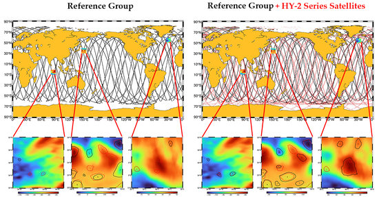
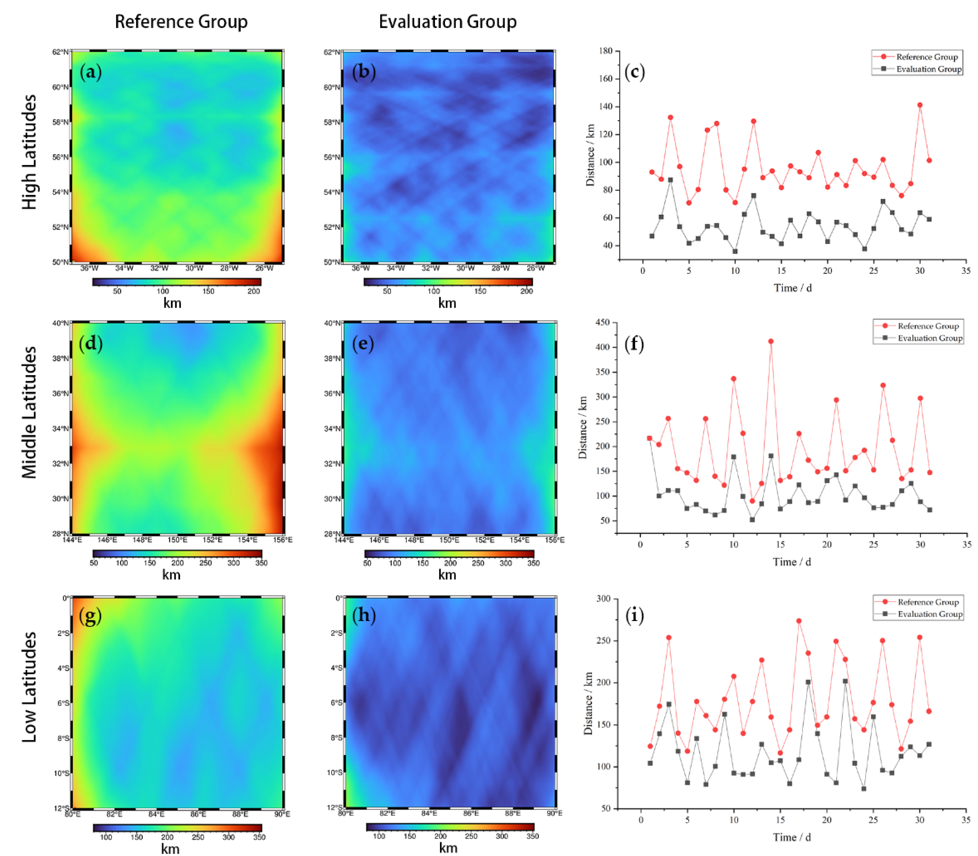
3.1. Comparing Along-Track Coverage

To assess the observation efficiency of HY-2 series satellites, we analyzed the distance to the nearest observation of the reference groups and evaluation groups at different latitudes. The shorter the distance to the nearest observation, the higher the density of orbital coverage. Generally, the orbital densities of three regions are, in descending order, high latitudes, middle latitudes and low latitudes. Regarding the spatial distribution of reference groups, it varies at different latitudes. At high latitudes (Figure 3a), the orbital coverage shows a decrease from top to bottom. At middle latitudes (Figure 3d), it is an hourglass shape, with a lower orbital coverage collected at the left and right edges. At low latitudes (Figure 3g), the orbital coverage is similar in all locations, except for low values at the north-west and south-west corners. In evaluation groups, the average distances to the nearest observation are decreased to 54 km at high latitudes (Figure 3b), 102 km at middle latitudes (Figure 3e) and 116 km at low latitudes (Figure 3h). The distance decreased by 43% at high latitudes (Figure 3c), 47% at middle latitudes (Figure 3f) and 35% at low latitudes (Figure 3i). Compared to the reference groups, it is a significant enhancement in the observation efficiency of evaluation groups.
It is worth noting that the increase in orbital density may reduce the tuned parameters in the OI algorithm. As can be seen from Table 2, for the same regions, the correlation scales of the evaluation groups decrease at both middle and high latitudes. When the along-ground tracks are sparse, observations cannot be effectively interpolated, which leads to a reduction in the accuracy of the gridded products. Thus, a suitable increase in correlation scales would prevent the results from containing fewer observations, improving the accuracy of the gridded products. However, correlation scales that are too large would smooth out the gridded products, leaving them lacking details. In summary, the selection of correlation scales is a compromise between the characteristics of the SSH field and the sampling capability of altimeter constellation.

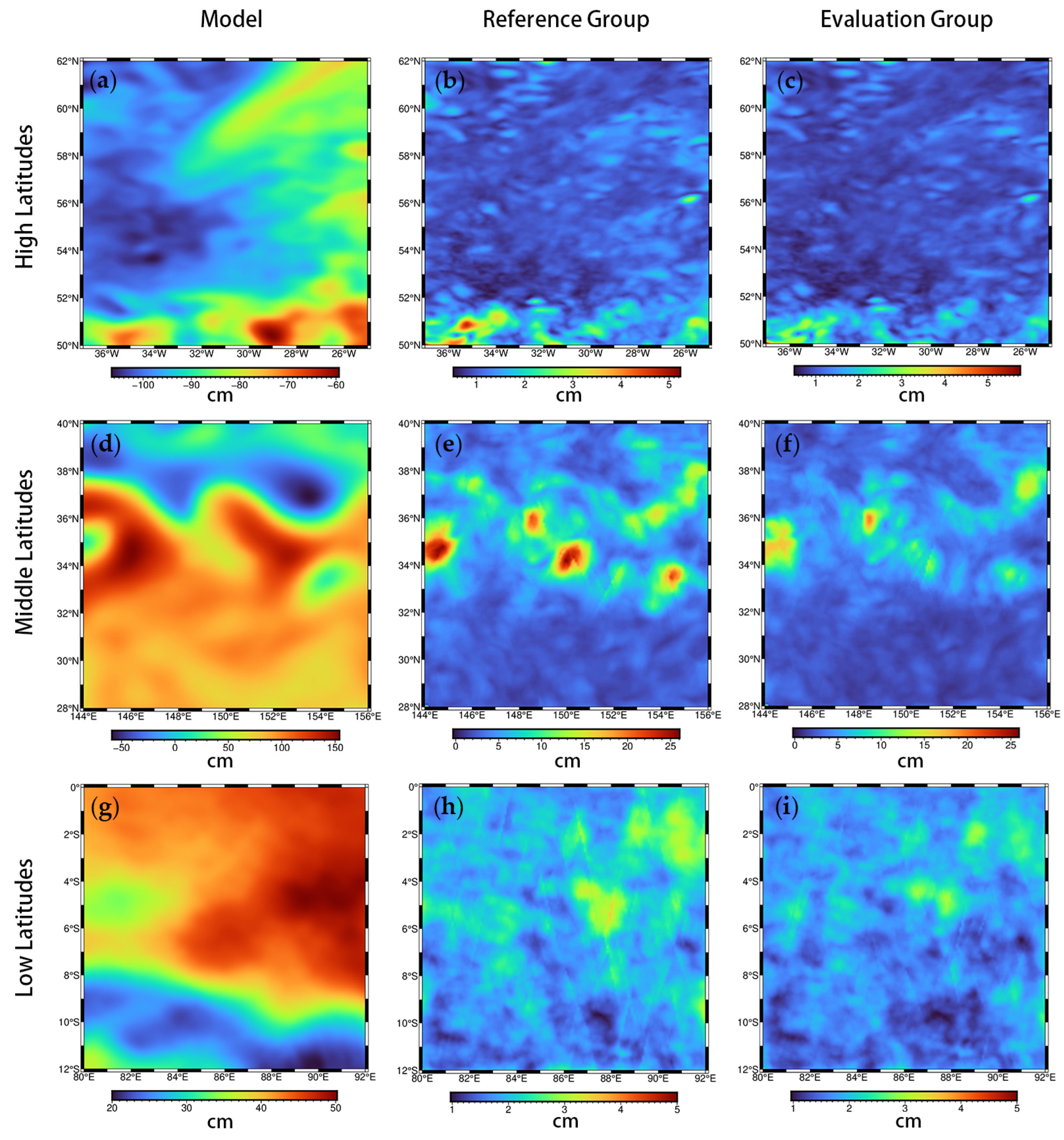
3.2. Comparing OI Gridded Product

We interpolated the altimetry satellite along ground tracks to gridded products by an OI analysis. Then, we tuned the parameters in the mapping procedure and obtained the best restoration of the gridded products.
The comparison results of the SSH fields are shown in Figure 4. The differences between the reference groups and evaluation groups are (Figure 4a) 1.16 cm and (Figure 4b) 1.07 cm at high latitudes; (Figure 4d) 5.04 cm and (Figure 4e) 3.87 cm at middle latitudes; and (Figure 4g) 1.95 cm and (Figure 4h) 1.75 cm at low latitudes. This indicates that the evaluation groups have an overall improvement of 8%, 23% and 10% at high, middle and low latitudes due to the addition of HY-2 series satellites. Similarly, the RMSE values for the reference groups and evaluation groups are 1.52 cm and 1.40 cm at high latitudes, 8.16 cm and 6.24 cm at middle latitudes, and 2.57 cm and 2.31 cm at low latitudes, with a difference of approximately 0.12 cm, 1.92 cm and 0.26 cm, respectively. It is worth noting that the errors mainly occurred at the transition regions between cold eddies and warm eddies, and the increase in orbital coverage had a pronounced enhanced effect on areas with high SSH variability.

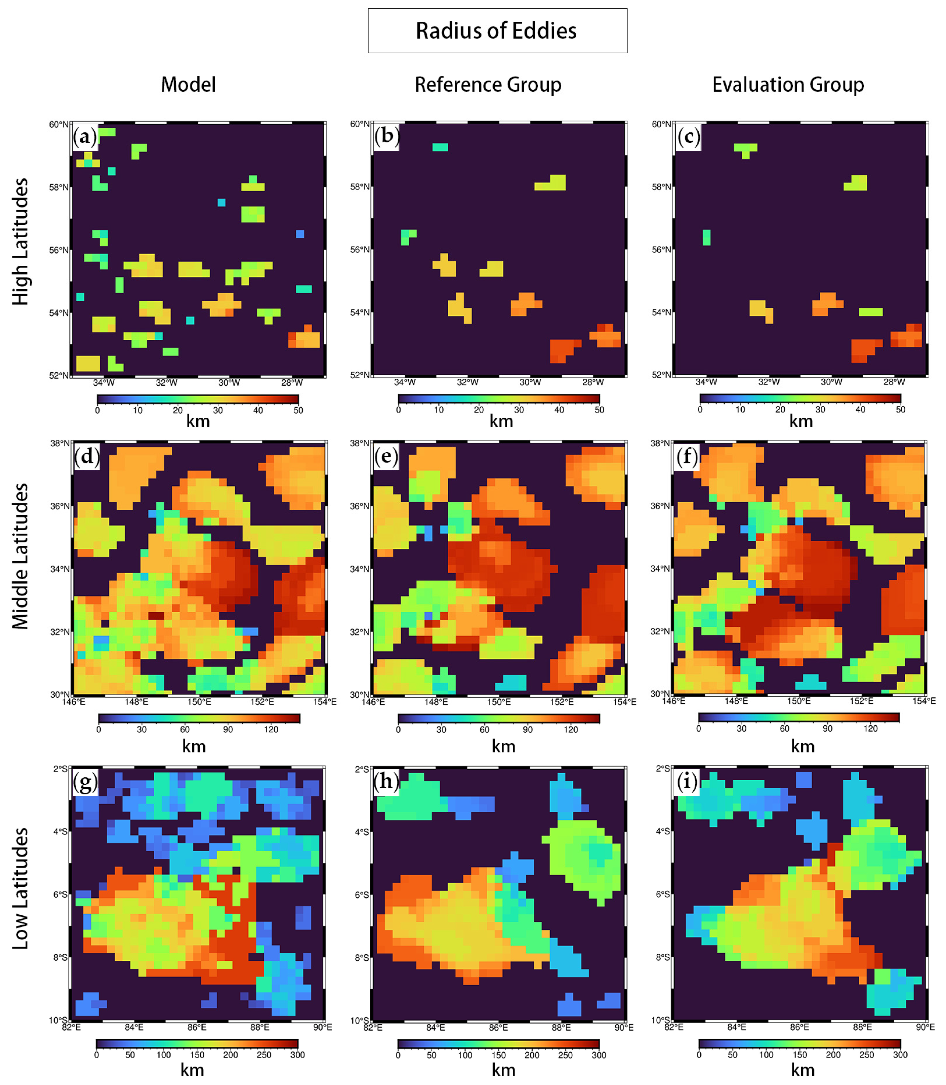
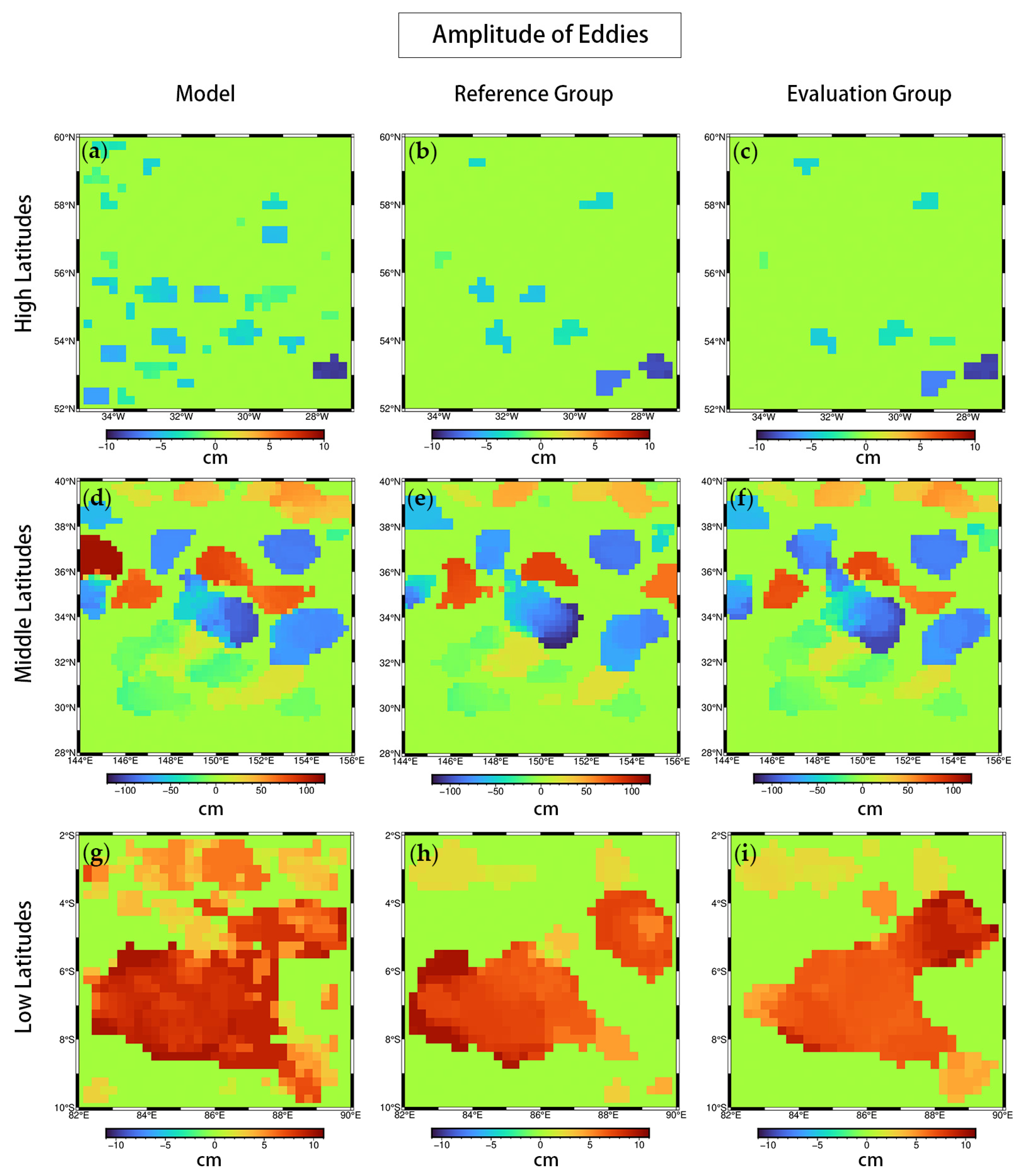
3.3. Comparing Identified Mesoscale Eddies

We applied the eddy identification algorithm to the model and two groups of gridded SSH products to identify mesoscale eddies at daily intervals. Due to the significant distortion of eddy fields at boundaries, we extended inward the eddy datasets with a scale of 2°. The resolution of synthetic data primarily affects eddies’ identification properties [43], thus, we ensured the same resolution of 0.08° × 0.08° in detection.
We selected eddy amount, radius and amplitude as the assessment criteria for mesoscale eddy identification. Eddy amount is defined as the number of mesoscale eddies counted. To identify only mesoscale eddies, the area of each individual eddy should be less than the area of a circle with a radius equal to the first baroclinic Rossby radius. Eddy effective radius is defined as R = S / π and S is the area enclosed by outlines. Eddy amplitude refers to the level of variation in eddy fluctuations.
It is illustrated in Table 3 that the statistics results of the eddies in the evaluation groups are similar to the eddies in the reference groups, with a slight improvement in eddy amount and radius, and poor performance in eddy amplitude. This may be related to the limited mapping improvement space from three to six satellites [8]. It is worth noting that the eddy datasets of the gridded SSH field show a serious incorrect estimation of the amount and radius of eddies at low latitudes. As can be seen from Figure 5c, there are a large number of smaller mesoscale eddies in the gridded products that are not captured correctly but over-identified some larger mesoscale eddies. This explains the incorrect statistical values of eddies at low latitudes.
The distribution of the eddy dataset attributes is statistically presented in Figure 5. It shows that smaller mesoscale eddies dominate high latitudes, with the radius distributed around 30 km (Figure 5a), while middle and low latitudes achieve a wider radius range than high latitudes, with the radius up to 140 km and 250 km, respectively (Figure 5b,c). The eddy amplitudes at high latitudes and low latitudes vary little and are distributed around 5 cm (Figure 5d–f). In contrast, the amplitudes at middle latitudes are more dispersed and the maximum value can reach 1.2 m (Figure 5e).
The distribution of eddies amount is shown in Figure 6, and the value of each grid represents the times of eddy identification in this location. High latitudes are distributed with smaller mesoscale eddies, which are sparse and discrete. Middle latitudes are dominated by mesoscale eddies throughout the region, which are large in number. While the center of low latitudes is clustered with eddy swarms, the margins are scattered with few mesoscale eddies. From the spatial distribution of eddy amount, HY-2 constellation alleviates eddies overestimation at middle latitudes (36–38°N, 152–154°E) and low latitudes (6–9°S, 84–86°E), as well as eddy underestimation at high latitudes (53–54°N, 28–29°W); middle latitudes (34–35°N, 152–154°E); and low latitudes (2–5°S, 84–87°E). However, it appears that there are a large number of small radius mesoscale eddies that are underestimated at low latitudes.
The distribution of eddy radius is shown in Figure 7, and the value of each grid represents the average eddy radius identified in this location. As can be seen from Figure 7, the spatial distribution of eddy radius is very well represented at high latitudes. However, for other regions, in the case of middle latitudes with a similar orbital density to low latitudes, middle latitudes have better eddy fields, but low latitudes do not reconstruct satisfactory eddy fields. At low latitudes, the eddy radius in gridded SSH fields is larger than in the model, indicating that some smaller mesoscale eddies are captured as bigger structures.
The distribution of eddy amplitude is shown in Figure 8, and the value of each grid represents the average eddy amplitude identified in this location. The spatial distribution of eddy amplitude variation is well reconstructed at both high latitudes and middle latitudes, while at low latitudes, both eddy datasets from gridded products are not able to capture enough eddies with small amplitude. However, the evaluation groups add more information on the amplitude of the eddy field than the reference groups to alleviate eddy underestimation.

4. Discussion

The results demonstrate the differences in the ability of altimetry satellites to improve the detection of eddies at different latitudes. On the one hand, although high latitudes have the greatest density of orbital coverage among three regions, it results in some eddies being underestimated because smaller mesoscale eddies (~30 km) are not easily captured. On the other hand, low and middle latitudes, where the orbital coverage is similar, produce quite different results. Specifically, the eddy fields are well identified at middle latitudes, while serious misidentification occurs at low latitudes, where the number of eddies is halved and their radius doubled.
To further investigate this problem, we selected several representative examples for transient observations. Figure 9 shows the eddies detected in three missions at different latitudes. We used eddies in the models as real eddies to compare the performance of eddies detected from synthetic SSH fields. A real eddy is considered to be captured if there is a similar shape and overlapping area to the eddies in the model.
The first feature illustrated in the figure is that the differences in orbital coverage could affect eddy detection. Specifically, both high latitudes and low latitudes have low sea surface variability and simpler eddy fields, while the orbital coverage at high latitudes is twice as high as orbital coverage at low latitudes. However, the result is that more than half of the eddies are correctly identified at high latitudes, with the eddy contours matching well with the model, but the area of eddies at low latitudes is generally exaggerated, with some smaller mesoscale eddies being identified as larger structures. The second feature illustrated in the figure is that the complexity of the eddy fields also affects the eddy identification results. To be specific, the orbital coverage is similar at middle latitudes and low latitudes, but due to the complexity of the eddy fields at middle latitudes, which have a higher number and larger radius of eddies, it instead produces better eddy matching results.
To better reflect the ability to identify real eddies, we analyzed the results of all real eddies captured from synthetic SSH fields and calculated eddy recognition rates and accuracy, as shown in Table 4. It can be seen that the eddy recognition rates are similar to the results obtained in Figure 9, with the highest values at middle latitudes, followed by high latitudes and finally, low latitudes. Specifically, eddy recognition rates and accuracy at middle latitudes are all around 50%, at high latitudes around 30%, while eddy recognition rates at low latitudes are only around 20% but can reach nearly half in accuracy. Then, we compared the differences in eddy recognition between the reference groups and evaluation groups in all regions. We found that under the background of an increase in orbital coverage of around 40% at three latitudes, the eddy recognition rates of the evaluation groups improved by 14% and 14% at high and low latitudes, and the accuracy rates of the evaluation groups improved by 16% and 7% at high and low latitudes.
In summary, it can be seen that the enhancement of eddy detection capability by HY-2 series satellites varies with regions. On the one hand, the orbital coverage is latitudinal and the enhancement is not equitable. For regions with similar eddy field complexity, such as the high latitudes and low latitudes in this paper, although they are both dominated by smaller mesoscale eddies, the probability of eddies being detected is enhanced by the increased orbital coverage. On the other hand, SSH field variability affects the accuracy of the eddy identification results. Under the same orbital coverage, such as the middle latitudes and low latitudes, smaller mesoscale eddies may more easily be distorted into larger structures by the mapping procedure [43], while the detection of larger mesoscale eddies is likely to be correctly captured. Thus, the accuracy of eddy detection seems like the result of a combination of the level of orbital coverage and the complexity of the eddy field.

5. Conclusions

In this paper, we analyzed the impact of HY-2 series satellites on the detection of mesoscale eddies by combining them with Jason-3, Sentinel-3A and Sentinel-3B missions at three latitude regions. We achieved this through a series of pseudo-observation experiments based on the geographical and temporal positions of altimetry satellite along ground tracks, using the outputs from the HYCOM model. Two altimetry satellite combinations were selected, namely, the reference group in the Jason-3+Sentinel-3A/B configuration and the evaluation group in the Jason-3+Sentinel-3A/B+HY-2B/C/D configuration. After generating synthetic SSH maps by an OI procedure, we applied the eddy identification algorithm to the original model outputs and the gridded products and then compared the eddy fields characteristics.
The result shows that the addition of HY-2 series satellites reduced the distance to the nearest observation by approximately 40% in all regions, with the distance to the nearest observation of 54 km at high latitudes, 102 km at middle latitudes and 116 km at low latitudes. Compared to the reference groups, the evaluation groups including HY-2 series satellites can effectively reduce synthetic product differences by 8%, 23% and 10% at high latitudes, middle latitudes, and low latitudes, which shows a great enhancement of satellite sampling capability. Moreover, the evaluation groups could alleviate eddy mis-estimation and add details to the eddy radius and amplitude. By comparing with eddies captured from model datasets, we found that the eddy recognition rate and accuracy were highest in the middle latitude regions, with values of around 50%, while the superior ability of HY-2 was demonstrated at high latitudes, with maximum improvements of 14% and 16% in eddy recognition rate and accuracy. This indicates that the enhancement of the eddy detection capability of HY-2 series satellites is not uniform. Both the level of orbital coverage and the complexity of the eddy field affect the results. Generally speaking, HY-2 series satellites can effectively improve the mapping capability of mesoscale eddies with a significant increase in orbital coverage.
This study provides a comprehensive assessment of the ocean observation capability of the HY-2 series satellites and offers a basis for the future scientific use of the HY-2 satellite data. However, in this paper, the detection performance of the HY-2 series satellites is only assessed in terms of mesoscale eddy detection, and the detection capability on the ocean dynamics environment still deserves further detailed study.

Author Contributions

Conceptualization, F.Y., J.Q. and G.C.; methodology, F.Y. and J.Q.; software, J.Q.; validation, F.Y., Y.J. and G.C.; formal analysis, F.Y.; investigation, J.Q.; resources, Y.J. and G.C.; data curation, J.Q.; writing—original draft preparation, J.Q.; writing—review and editing, F.Y. and G.C.; visualization, J.Q.; supervision, F.Y.; project administration, F.Y. and G.C.; funding acquisition, F.Y. and G.C. All authors have read and agreed to the published version of the manuscript.

Funding

This research was funded by the following programs: (1) the National Key R&D Program of China, (Grant No. 2019YFD0901001); (2) the Marine S&T Fund of Shandong Province for the Pilot National Laboratory for Marine Science and Technology (Qingdao) (Grant No. 2021WHZZB1705); (3) the Marine S&T Fund of Shandong Province for the Pilot National Laboratory for Marine Science and Technology (Qingdao) (Grant No. 2022QNLM050301).

Data Availability Statement

Not applicable.

Acknowledgments

We are thankful to the NSOAS, NOAA, NASA, CNES, EUMETSAT, ESA, CLS, CMEMS, DUACS and HYCOM for providing the data.

Conflicts of Interest

The authors declare no conflict of interest.

Abbreviations

The following abbreviations are used in this manuscript:
HY-2Haiyang-2
HY-2BHaiyang-2B
HY-2CHaiyang-2C
HY-2DHaiyang-2D
NSOASNational Satellite Ocean Application Service
NOAANational Oceanic and Atmospheric Administration
NASANational Aeronautics and Space Administration
CNESCenter National ďEtudes Spatiales
EUMETSATEuropean Organization for Exploitation of Meteorological Satellites
ESAEuropean Space Agency
HYCOMHybrid Coordinate Ocean Model
DUACSData Unification and Altimeter Combination System
CLSCollect Localization Satellites
CMEMSCopernicus Marine and Environment Monitoring Service
SLASea Level Anomaly
OIOptimal Interpolation
SSHSea Surface Height
CLSCollect Localization Satellites

References

  1. Zhen, Y.C.; Tandeo, P.; Leroux, S.; Metref, S.; Penduff, T.; Le Sommer, J. An Adaptive Optimal Interpolation Based on Analog Forecasting: Application to SSH in the Gulf of Mexico. J. Atmos. Ocean. Tech. 2020, 37, 1697–1711. [Google Scholar] [CrossRef]
  2. Taburet, G.; Sanchez-Roman, A.; Ballarotta, M.; Pujol, M.I.; Legeais, J.F.; Fournier, F.; Faugere, Y.; Dibarboure, G. DUACS DT2018: 25 years of reprocessed sea level altimetry products. Ocean Sci. 2019, 15, 1207–1224. [Google Scholar] [CrossRef]
  3. Chelton, D.B.; Schlax, M.G.; Samelson, R.M.; de Szoeke, R.A. Global observations of large oceanic eddies. Geophys. Res. Lett. 2007, 34. [Google Scholar] [CrossRef]
  4. Samelson, R.M.; Schlax, M.G.; Chelton, D.B. Global observations of nonlinear mesoscale eddies. J. Phys. Oceanogr. 2014, 44, 2588–2589. [Google Scholar] [CrossRef]
  5. Fu, L.L.; Ubelmann, C. On the Transition from Profile Altimeter to Swath Altimeter for Observing Global Ocean Surface Topography. J. Atmos. Ocean. Tech. 2014, 31, 560–568. [Google Scholar] [CrossRef]
  6. Gandin, L.S. Objective Analysis of Meteorological Fields. Isr. Program Sci. Transl. 1963, 286. [Google Scholar]
  7. Ducet, N.; Le Traon, P.Y.; Reverdin, G. Global high-resolution mapping of ocean circulation from TOPEX/Poseidon and ERS-1 and-2. J. Geophys. Res. Ocean. 2000, 105, 19477–19498. [Google Scholar] [CrossRef]
  8. Le Traon, P.Y.; Dibarboure, G. Mesoscale mapping capabilities of multiple-satellite altimeter missions. J. Atmos. Ocean. Tech. 1999, 16, 1208–1223. [Google Scholar] [CrossRef]
  9. Koblinsky, C. Oceans and climate change: The future of spaceborne altimetry. Trans. Am. Geophys. Union 1992, 73, 403. [Google Scholar] [CrossRef]
  10. Morrow, R.; Le Traon, P.Y. Recent advances in observing mesoscale ocean dynamics with satellite altimetry. Adv. Space Res. 2012, 50, 1062–1076. [Google Scholar] [CrossRef]
  11. Le Traon, P.Y.; Dibarboure, G. Velocity mapping capabilities of present and future altimeter missions: The role of high-frequency signals. J. Atmos. Ocean. Tech. 2002, 19, 2077–2087. [Google Scholar]
  12. Fu, L.L.; Christensen, E.J.; Yamarone, C.A.; Lefebvre, M.; Menard, Y.; Dorrer, M.; Escudier, P. TOPEX/POSEIDON mission overview. J. Geophys. Res. Ocean. 1994, 99, 24369–24381. [Google Scholar]
  13. Wang, Z.X.; Zou, J.H.; Zhang, Y.G.; Stoffelen, A.; Lin, W.M.; He, Y.J.; Feng, Q.; Zhang, Y.; Mu, B.; Lin, M.S. Intercalibration of Backscatter Measurements among Ku-Band Scatterometers Onboard the Chinese HY-2 Satellite Constellation. Remote Sens. 2021, 13, 4783. [Google Scholar]
  14. Guo, Q. China Launches HY-2B Satellite Atop a LM-4B. Aerosp. China 2018, 19, 59. [Google Scholar]
  15. Yueming, R. LM-4B Successfully Launched HY-2C Satellite. Aerosp. China 2020, 21, 56. [Google Scholar]
  16. Zou, J.; Mu, B.; Bao, Q.; Wang, Z.; Lang, S.; Yang, S.; Lin, M. Calibration and Validation of Scatterometer Product of CFOSAT and HY-2 Series Satellites. In Proceedings of the 2021 IEEE International Geoscience and Remote Sensing Symposium IGARSS, Brussels, Belgium, 11–16 July 2021; pp. 8138–8141. [Google Scholar]
  17. Guo, J.Y.; Wang, G.Z.; Guo, H.Y.; Lin, M.S.; Peng, H.L.; Chang, X.T.; Jiang, Y.M. Validating Precise Orbit Determination from Satellite-Borne GPS Data of Haiyang-2D. Remote Sens. 2022, 14, 2477. [Google Scholar]
  18. Lin, M.S.; Jia, Y.J. Past, Present and Future Marine Microwave Satellite Missions in China. Remote Sens. 2022, 14, 1330. [Google Scholar]
  19. Zhou, X.; Yang, L.; Lin, M.; Lei, N.; Tang, Q.; Mu, B. Absolute calibration of HY-2, Jason-2 and Saral/AltiKa from China in-situ calibration site: Qian Li Yan. In Proceedings of the 2015 IEEE International Geoscience and Remote Sensing Symposium (IGARSS), Milan, Italy, 26–31 July 2015; pp. 3659–3662. [Google Scholar]
  20. Liu, Q.X.; Babanin, A.V.; Guan, C.L.; Zieger, S.; Sun, J.; Jia, Y.J. Calibration and Validation of HY-2 Altimeter Wave Height. J. Atmos. Ocean. Tech. 2016, 33, 919–936. [Google Scholar]
  21. Jia, Y.; Lin, M.; Zhang, Y. Current status of the HY-2A satellite radar altimeter and its prospect. In Proceedings of the Geoscience & Remote Sensing Symposium, Quebec City, QC, Canada, 3–18 July 2014. [Google Scholar]
  22. Mingsen, L.; Xingwei, J. Ocean observation from Haiyang satellites. Chin. J. Space Sci. 2020, 40, 898–907. [Google Scholar]
  23. Xingwei, J.; Mingsen, L. Ocean Observation from Haiyang Satellites: 2012–2014. Chin. J. Space Sci. 2014, 34, 710–720. [Google Scholar]
  24. Pascual, A.; Faugère, Y.; Larnicol, G.; Le Traon, P.Y. Improved description of the ocean mesoscale variability by combining four satellite altimeters. Geophys. Res. Lett. 2006, 33. [Google Scholar] [CrossRef] [Green Version]
  25. Le Traon, P.; Faugère, Y.; Hernandez, F.; Dorandeu, J.; Mertz, F.; Ablain, M. Can we merge GEOSAT follow-on with TOPEX/Poseidon and ERS-2 for an improved description of the ocean circulation? J. Atmos. Ocean. Tech. 2003, 20, 889–895. [Google Scholar]
  26. Pujol, M.I.; Faugere, Y.; Taburet, G.; Dupuy, S.; Pelloquin, C.; Ablain, M.; Picot, N. DUACS DT2014: The new multi-mission altimeter data set reprocessed over 20 years. Ocean Sci. 2016, 12, 1067–1090. [Google Scholar]
  27. Dibarboure, G.; Renaudie, C.; Pujol, M.I.; Labroue, S.; Picot, N. A demonstration of the potential of Cryosat-2 to contribute to mesoscale observation. Adv. Space Res. 2012, 50, 1046–1061. [Google Scholar]
  28. Dibarboure, G.; Lamy, A.; Pujol, M.I.; Jettou, G. The Drifting Phase of SARAL: Securing Stable Ocean Mesoscale Sampling with an Unmaintained Decaying Altitude. Remote Sens. 2018, 10, 1051. [Google Scholar]
  29. Donlon, C.J.; Cullen, R.; Giulicchi, L.; Vuilleumier, P.; Francis, C.R.; Kuschnerus, M.; Simpson, W.; Bouridah, A.; Caleno, M.; Bertoni, R.; et al. The Copernicus Sentinel-6 mission: Enhanced continuity of satellite sea level measurements from space. Remote Sens. Environ. 2021, 258, 112395. [Google Scholar]
  30. Vaze, P.; Neeck, S.; Bannoura, W.; Green, J.; Wade, A.; Mignogno, M.; Zaouche, G.; Couderc, V.; Thouvenot, E.; Parisot, F. The jason-3 mission: Completing the transition of ocean altimetry from research to operations. In Proceedings of the Conference on Sensors, Systems, and Next-Generation Satellites XIV, Toulouse, France, 20–23 September 2010. [Google Scholar]
  31. Mavrocordatos, C.; Berruti, B.; Aguirre, M.; Drinkwater, M. The Sentinel-3 mission and its Topography element. In Proceedings of the IEEE International Geoscience and Remote Sensing Symposium (IGARSS), Barcelona, Spain, 23–27 July 2007; pp. 3529–3532. [Google Scholar]
  32. Chassignet, E.P.; Huriburt, H.E.; Smedstad, O.M.; Halliwell, G.R.; Hogan, P.J.; Wallcraft, A.J.; Bleck, R. Ocean prediction with the hybrid coordinate ocean model (HYCOM). In Proceedings of the International Summer School of Oceanography, Agelonde in Lalonde-Les Maures, Agelonde, France, 20 September–1 October 2004; pp. 413–426. [Google Scholar]
  33. Meyers, G.; Phillips, H.; Smith, N.; Sprintall, J. Space and time scales for optimal interpolation of temperature—Tropical Pacific Ocean. Prog. Oceanogr. 1991, 28, 189–218. [Google Scholar]
  34. Le Traon, P.Y.; Ogor, F. ERS-1/2 orbit improvement using TOPEX/POSEIDON: The 2 cm challenge. J. Geophys. Res. Ocean. 1998, 103, 8045–8057. [Google Scholar]
  35. Dong, C.M.; Nencioli, F.; Liu, Y.; McWilliams, J.C. An Automated Approach to Detect Oceanic Eddies From Satellite Remotely Sensed Sea Surface Temperature Data. IEEE Geosci. Remote Sens. Lett. 2011, 8, 1055–1059. [Google Scholar] [CrossRef]
  36. Kurian, J.; Colas, F.; Capet, X.; McWilliams, J.C.; Chelton, D.B. Eddy properties in the California current system. J. Geophys. Res. Ocean. 2011, 116. [Google Scholar] [CrossRef]
  37. Li, Q.Y.; Sun, L.; Lin, S.F. GEM: A dynamic tracking model for mesoscale eddies in the ocean. Ocean Sci. 2016, 12, 1249–1267. [Google Scholar]
  38. Faghmous, J.H.; Le, M.; Uluyol, M.; Kumar, V.; Chatterjee, S. A parameter-free spatio-temporal pattern mining model to catalog global ocean dynamics. In Proceedings of the IEEE 13th International Conference on Data Mining (ICDM), Dallas, TX, USA, 7–10 December 2013; pp. 151–160. [Google Scholar]
  39. Nencioli, F.; Dong, C.M.; Dickey, T.; Washburn, L.; McWilliams, J.C. A Vector Geometry-Based Eddy Detection Algorithm and Its Application to a High-Resolution Numerical Model Product and High-Frequency Radar Surface Velocities in the Southern California Bight. J. Atmos. Ocean. Tech. 2010, 27, 564–579. [Google Scholar]
  40. Meng, Y.; Liu, H.L.; Lin, P.F.; Ding, M.R.; Dong, C.M. Oceanic mesoscale eddy in the Kuroshio extension: Comparison of four datasets. Atmos. Ocean. Sci. Lett. 2021, 14, 100011. [Google Scholar]
  41. Escudier, R.; Renault, L.; Pascual, A.; Brasseur, P.; Chelton, D.; Beuvier, J. Eddy properties in the Western Mediterranean Sea from satellite altimetry and a numerical simulation. J. Geophys. Res. Ocean. 2016, 121, 3990–4006. [Google Scholar]
  42. Martinez-Moreno, J.; Hogg, A.M.; Kiss, A.E.; Constantinou, N.C.; Morrison, A.K. Kinetic Energy of Eddy-Like Features From Sea Surface Altimetry. J. Adv. Modeling Earth Syst. 2019, 11, 3090–3105. [Google Scholar]
  43. Amores, A.; Jordà, G.; Arsouze, T.; Le Sommer, J. Up to what extent can we characterize ocean eddies using present-day gridded altimetric products? J. Geophys. Res. Ocean. 2018, 123, 7220–7236. [Google Scholar]
Figure 1. Workflow of the evaluation methodology.
Remotesensing 14 04262 g001
Figure 2. January 2019 of (a) DUACS DT2018 sea level anomaly (SLA) products; (b) SLA obtained by our optimal interpolation (OI) analysis; and (c) differences between two datasets. Unit of SLA in cm.
Remotesensing 14 04262 g002
Figure 3. Orbital coverage distribution of reference groups and evaluation groups at (a,b) high latitudes, (d,e) middle latitudes, and (g,h) low latitudes. The value of each figure is the distance to the nearest along-track observation, which is used to represent orbital coverage. Time series of daily orbital coverage of reference groups and evaluation groups at (c) high latitudes, (f) middle latitudes, and (i) low latitudes. Unit of distance is km and unit of time is day.
Remotesensing 14 04262 g003
Figure 4. Sea surface height (SSH) products for models, reference groups and evaluation groups at (ac) high latitudes, (df) middle latitudes, and (gi) low latitudes. Unit of SSH in cm.
Remotesensing 14 04262 g004
Figure 5. Statistical histograms of radius at (a) high latitudes, (b) middle latitudes, and (c) low latitudes. Statistical histograms of amplitude at (d) high latitudes, (e) middle latitudes, and (f) low latitudes. Red boxes are for the model datasets, blue boxes for reference groups and green boxes for evaluation groups. Unit of radius is km and unit of amplitude is m.
Remotesensing 14 04262 g005
Figure 6. Distribution of eddies amount generated from models, reference groups and evaluation groups at (ac) high latitudes, (df) middle latitudes, and (gi) low latitudes. The resolution of the grid is 0.25° × 0.25°.
Remotesensing 14 04262 g006
Figure 7. Distribution of eddies radius generated from models, reference groups and evaluation groups at (ac) high latitudes, (df) middle latitudes, and (gi) low latitudes. The resolution of the grid is 0.25° × 0.25°. Unit of radius in km.
Remotesensing 14 04262 g007
Figure 8. Distribution of eddies amplitude generated from models, reference groups and evaluation groups at (ac) high latitudes, (df) middle latitudes, and (gi) low latitudes. The resolution of the grid is 0.25° × 0.25°. Unit of amplitude in cm.
Remotesensing 14 04262 g008
Figure 9. Examples of eddies identified on models, reference groups and evaluation groups at (ac) high latitudes, (df) middle latitudes, and (gi) low latitudes. The background color is from SSH fields of different datasets on the current day. The centers of eddies detected in model datasets are shown as black crosses and their contours as thin black lines. The centers of eddies detected in the reference groups and evaluation groups are black circles and their contours are bold black lines. Unit of SSH in cm.
Remotesensing 14 04262 g009
Table 1. Altimetry satellite information of HY-2B/C/D, Jason-3 and Sentinel-3A/B.
SatelliteAgencyLaunchInclinationSun-
Synchronous
WavebandRepetitive
HY-2BNSOAS2018.1099.3°YesKu/C14day
HY-2CNSOAS2020.0966°NoKu10day
HY-2DNSOAS2021.0566°NoKu10day
Jason-3NOAA&NASA&
CNES&EUMETSAT
2016.0166°NoKu/C10day
Sentinel-3ANOAA&NASA2016.0298.6°YesKu/C27 day
Sentinel-3BNOAA&NASA2018.0498.6°YesKu/C27 day
Table 2. Tuned spatial scale L x and temporal scale L t for reference groups and evaluation groups at high, middle and low latitudes. Unit of L x is km and unit of L t is day.
Reference GroupEvaluation Group
High
Latitudes
Middle
Latitudes
Low
Latitudes
High
Latitudes
Middle
Latitudes
Low
Latitudes
L x /km801001207090120
L t /day773333
Table 3. Eddy amount, radius and amplitude for models, reference groups and evaluation groups at high, middle and low latitudes. Unit of radius is km and unit of amplitude is m.
High LatitudesMiddle LatitudesLow Latitudes
ModelReference GroupEvaluation GroupModelReference GroupEvaluation GroupModelReference GroupEvaluation Group
Ed. Amount1141101082913063041175255
Ed. Radius/km25.1032.2032.6469.0473.2072.4256.19109.03104.96
Ed. Amplitude/cm−4.15−4.67−4.70−10.53−17.64−21.624.265.114.84
Table 4. Eddy recognition rates and accuracy for reference groups and evaluation groups in different latitudes. Eddy recognition rate is equal to the number of real eddies captured in the gridded product divided by its total number of eddies, and eddy recognition accuracy is equal to the number of real eddies captured in the gridded product divided by the total number of eddies in its corresponding model.
Eddy Recognition Rate/%Eddy Recognition Accuracy/%
High
Latitudes
Middle
Latitudes
Low
Latitudes
High
Latitudes
Middle
Latitudes
Low
Latitudes
Reference Group30.9755.3518.8031.8255.8742.31
Evaluation Group35.4052.5621.3737.0455.6645.45
Publisher’s Note: MDPI stays neutral with regard to jurisdictional claims in published maps and institutional affiliations.

