Article

A Generalized Labeled Multi-Bernoulli Filter Based on Track-before-Detect Measurement Model for Multiple-Weak-Target State Estimate Using Belief Propagation

1
School of Electronic Engineering, Xi’an University of Posts & Telecommunications, Xi’an 710121, China
2
National Lab of Radar Signal Processing, Xidian University, Xi’an 710071, China
*
Author to whom correspondence should be addressed.
Remote Sens. 2022, 14(17), 4209; https://doi.org/10.3390/rs14174209
Submission received: 2 August 2022 / Revised: 20 August 2022 / Accepted: 23 August 2022 / Published: 26 August 2022

Abstract

:
In this paper, we propose the specific recursion formula for the generalized labeled multi-Bernoulli filter based on the track-before-detect strategy (GLMB-TBD) using a belief propagation algorithm. The proposed method aims to track multiple weak targets with superior performance. Compared to the Murty algorithm-based and Gibbs sampling-based implementation of GLMB-TBD filter, the proposed algorithm improves the tracking accuracy of multiple weak targets without pruning operation to preserve the relevant association information. The superior performance in tracking accuracy of the algorithm is validated for simulated scenarios using OSPA(2) metric. More importantly, the simulation results demonstrate that the proposed algorithm outputs both the Gibbs sampling-based version and Murty algorithm-based version in computational cost due to linear complex in the number of both Bernoulli components and measurements.

1. Introduction

The object of the multi-target tracking is to jointly estimate the unknown number of moving targets and their time-varying trajectories from measurements provided by remote sensors. Traditional approaches to multi-target tracking include the joint probabilistic data association (JPDA) [1] and multiple hypothesis tracking (MHT) [2]. A more recent class of multi-target tracking methods, namely random finite set (RFS) has attracted significant attention due to its general systematic framework of multi-target systems. The RFS-based method provides the basis for the development of novel filters without specific data association operation such as the probability hypothesis density (PHD) filter [3], cardinalized PHD (CPHD) filter [4,5,6,7], and multi-Bernoulli (MB) filter. These filters, in principle, are not multi-target trackers because their states are estimated, not trajectories. The introduction of the generalized labeled multi-Bernoulli (GLMB) filter has resulted in the development of the firstly tractable and mathematically principled RFS-based multi-target tracker [8,9,10,11,12,13,14].
In the standard detect-before-track approach, multi-target tracking is usually performed on preprocessed data. Compressing information from the raw measurement into finite set of points is very effective for a wide range of applications when computing and memory resources are limited. However, this approach may not be suitable for applications with low signal-to-noise ratio (SNR) since echo information loss will become significant for subsequent multi-target tracking. The track-before-detect (TBD) paradigm can work well in the scenario with low SNR due to preserving the raw echo data [15,16,17,18,19,20]. Early TBD methods are formulated as batch methods using the Hough transform, maximum likelihood estimation and dynamic programming [21]. Its online implementation, however, is cumbersome due to the impracticality of state-space discretization in realistic problems and its requirement for high-dimensional maximization. Finally, the recursive single-frame TBD approach was explored to obtain the superior tracking performance of multiple weak targets. Specifically, the optimal Bayesian solution was formulated as the TBD method based on GLMB filter (GLMB-TBD) [17]. Unfortunately, the posterior density for GLMB-TBD filter is not of the same type of GLMB RFS, whereas the update density for GLMB-TBD filter is labeled RFS mixture density but no longer GLMB form even if the predicted density follows a GLMB distribution [17,19]. That is to say, the GLMB on the state space is not necessarily conjugated prior to the TBD observation model. In general, the multi-target mixture density is intractable as a mathematical analytic solution, resulting in difficultly bein applied in practice. In [17], an approximation based on Kullback–Leibler divergence is adopted to develop a tractable recursive GLMB filter for a generic observation model.
Multi-target tracking is complicated mainly due to the unknown association between measurements and targets. In [22], a graphical model formulation of data association is presented, and an approximate inference method based on belief propagation is used to obtain estimation of marginal association probabilities. In [23], this belief propagation (BP) scheme is used to obtain a fast labeled multi-Bernoulli filter where the GLMB RFS is reformulated in terms of a joint association distribution. In [24], the self-tuning algorithm for multiple sensors is developed for tracking multiple targets using a belief propagation. In [25], an efficient implementation of GLMB filter based on Gibbs sampling is presented with linear complexity both in the number of measurements and in the number of samples. This paper incorporates a variant of the belief propagation scheme to solve the probabilistic association problem in the GLMB-TBD filter.
This paper focuses on tracking the problem of multiple weak targets based on the single-frame recursive TBD algorithm with GLMB RFS. A fast approximation calculation of the marginal association probability using belief propagation algorithm is presented to obtain the specific recursion formulate for the GLMB-TBD filter. Contrary to the traditional GLMB-TBD filter implementations based on Murty’s algorithm and Markov chain Monte Carlo techniques, the GLMB-TBD filter based on belief propagation algorithm can achieve superior tracking accuracy due to preserving the relevant association information. In particular, the belief propagation-based implementation algorithm is highly computationally feasible with linear complexity in the number of Bernoulli components in GLMB posterior, while it is better than Gibbs sampling-based with, at best, quadratic scales.
The rest of this paper is organized as follows. The backgrounds on GLMB RFS and GLMB filter based on the image pixeled TBD model are provided in Section 2. An efficient implementation of the GLMB-TBD filter based on belief propagation algorithm is developed in Section 3. Simulation results follow in Section 4. The discussion on the performance of the BP-based solution is presented in Section 5. Concluding remarks and future research are stated in Section 6.

2. Background

This section provides background on the GLMB-TBD implementation pertinent to the formulation of the proposed multiple-weak-target tracking problem.

2.1. Likelihood Function Based on Pixel TBD Measurement Model

In this section, we develop the multi-target estimation problem based labeled RFS with the pixeled TBD measurement model. The tracking approaches based on the GLMB model under the standard measurement model have been well investigated [26]. One remarkable development is that the GLMB family of posteriors are conjugated prior with respect to the standard multi-target likelihood. The TBD measurement model with the pixeled-image sensor is studied in this paper. The physical scenario considered in this work is illustrated in Figure 1. A target-detect-track radar is used for monitoring a given area with the maximum radar range R and angular extension Θ . The radar positioned at origin x 0 , y 0 receives the echo signal with three dimensional measurements in a "range-Doppler-angle" plane using the pixeled-image-TBD sensor. The collected data at the k frame is processed through the matched filtering, pulsed Doppler processing and envelope detection to yield
z k = z k i , j , ϑ , i = 1 , 2 , , N r , j = 1 , 2 , , N d , ϑ = 1 , 2 , , N θ
where z k i , j , ϑ denotes the intensity information recorded in i , j , ϑ cell at the k th frame. The received intensity information is the energy of the echo signal, i.e., z k i , j , ϑ = z k A i , j , ϑ 2 , where z k A i , j , ϑ denotes the complex signal with
z k A i , j , ϑ = z ^ k A i , j , ϑ + v k i , j , ϑ = x X 1 C x i A x h A i , j , ϑ + v k i , j , ϑ
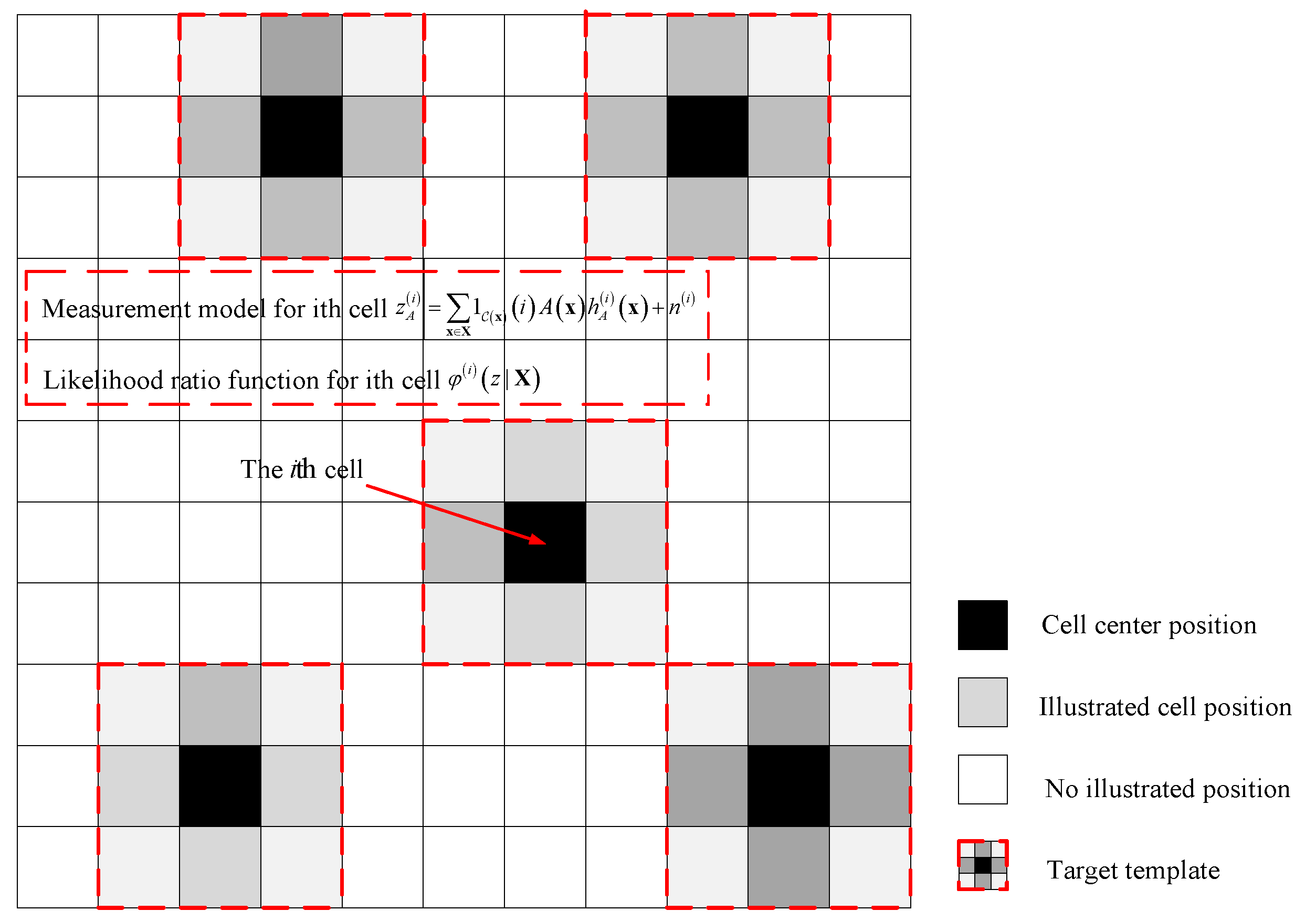
where the measurement noise v k i , j , ϑ is assumed to be white circularly symmetric complex Gaussian process with zero mean and variance 2 σ v 2 . As shown in Figure 2, a target with the state x X illuminates a set of cells, usually referred to the illuminated template. The template C x is defined as the set of image pixels whose center is positioned at a certain distance from the position of the target. The certain distance is referred to be the influenced region of the illustrated template. Hence, the different templates would have the different influenced regions yielding different pixeled measurement models. For example, the effective template 3   pix × 3   pix pixeled square region contributes to nine pixeled grids with adjacent regions. That is to say, the pixeled cells in the template are illustrated by a target, and the illustrated cell position is defined by the center point of the template.
The complex echo in echo signal z ^ k A i , j , ϑ for the target of a Swerling 0 is constant in modulus
A x =   A   ¯ e j θ , θ U 0 , 2 π
The surveillance region based on pixeled-image-TBD sensor is divided into N r × N d × N θ cells, where N r = R / Δ r , N d = D / Δ d + 1 and N θ = Θ / Δ θ denote the number of ranges, Doppler and angle cells, respectively. The range resolution Δ r = c / 2 B is determined by the waveform bandwidth B . The Doppler resolution Δ d = 1 / T is dependent on the coherent processing interval (CPI) T . The angle resolution Δ θ is given by the 3 dB beamwidth.
Given the radar original position x o = x o , y o and target state x k = x k , x ˙ k , y k , y ˙ k T 4 in the Cartesian coordinate. A target with state x k illustrates several cells of its surroundings denoted by C x k . Within the illustrating template of the target with state x k , the intensity contribution to the i , j , ϑ cell follows a point spread function with
h A i , j , ϑ x k = exp r i r k 2 2 Δ r L r d j d k 2 2 Δ d L d θ ϑ θ k 2 Δ θ L θ
where L r , L d and L θ denote loss coefficient in the three-dimension measurement. The unambiguous polar state p k = r k , d k , θ k T is given by
r k = x k x o 2 + y k y o 2
d k = x ˙ k , y ˙ k x k x o y k y o / x k x o 2 + y k y o 2
θ k = arctan y k y o / x k x o
The measurement z k i , j , ϑ in each cell follows a non-central chi-squared distribution with two degrees of freedom and non-centrality parameter z ^ A i , j , ϑ , i.e., z k i , j , ϑ H 1 Rice z ^ A i , j , ϑ , 1 . In the case with no target, it simplifies to a central chi-squared distribution with two degrees of freedom, i.e., z k i , j , ϑ H 0 Rayleigh σ v 2 . Consequently, the likelihood ratio for the cell i , j , ϑ based on pixeled-image TBD model is given by
φ z k i , j , ϑ | X = exp z ^ A i , j , ϑ 2 I 0 z k i , j , ϑ z ^ A i , j , ϑ
where I 0 denotes the modified Bessel function. Assume that measurements in each cell are independently distributed conditioned on the multi-target state X . As a result, the multi-target likelihood for pixeled-image TBD model is given by
g k Z | X i , j , ϑ x X C x φ z k i , j , ϑ | X
Note that multi-target likelihood (9) accommodates super-positional measurement, not only when targets are nearby in the state space, but more generally when they are closely-spaced in the measurement space. Subsequently, the pixeled-image TBD measurement model will be applied into the GLMB filter to achieve superior tracking performance of the low-SNR targets.

2.2. Generalized Labeled Multi-Bernoulli Filter Based on TBD Model

The multi-target estimation problem is formulated as a Bayesian framework by modeling the collection of states and measurement as a finite set. The tracking problem is concerned with calculating the posterior distribution of the random finites set of states given the image observation. Computing the posterior of a random finite set is intractable in general, even for the special case of superpositional measurement models where the image observation is the sum of the observations generated by individual states and noise.
If the multi-target prior is a labeled RFS density with the GLMB form, then the posterior density with respect to the standard dynamic transition model and generic observation model, especially the image pixeled TBD model, is given by
π X k = Δ X k I , ξ , I + , θ + w I + , ξ , θ + δ I + L X k p ξ , θ + x , l
where I F L , ξ Ξ , I + F L + , θ + Θ + , and
w I + , ξ , θ + I w I , ξ 1 Θ + I + θ + 1 P ¯ S ξ I I + P ¯ S ξ I I + 1 r B , + B + I + r B , + B + I + η I
P ¯ S ξ l = p ξ x , l P S x , l d x
p ξ , θ + x , l = g Z | X p + ξ X / η I
p + ξ x + , l + = 1 L l + P S , l + f + x + | , l + , p ξ , l + P ¯ S ξ l + + 1 B + l + p B , + x + , l +
η l 1 , l 2 , , l n = g Z | x 1 , l 1 , , x n , l n j = 1 n p + l 1 , , l n x j , l j d x 1 , , x n
It is observed from (10) that the posterior density at next time becomes p ξ , θ + X | Z after the update each multi-target exponential p + ξ X with respect to image pixeled TBD observation model. In general, the posterior in (10) is not a GLMB density. Hence, the posterior density is not conjugated with regard to the image pixeled TBD observation model at all. Although the reference [26] has indicated that the family of labeled RFS mixture densities can be regarded as conjugate prior with respect to generic observation model, it is numerically intractable, albeit with formal closure under Bayesian recursion.
It is necessary for the recursive tracker to approximate the labeled mixture prior by a GLMB form. Essentially, the prior of GLMB form can be obtained by marginalizing the labeled mixture densities (joint densities) post-update. In order to bring the posterior density back to the required GLMB form, the posterior in (10) can be translated into the product form of marginalization of the labeled mixture posterior density, i.e.,
π X k = Δ X k I + F L + θ k Θ I + w I + , θ k δ I + L X k x k , l X k s l , θ k l x k
The weight w I + , θ k and spatial density s l , θ k l are normalization factors, and can be expressed by
w L , θ k l L k \ L 1 r k | k 1 l l L r k | k 1 l η l , θ k l
where
η k l , m = 1 p D x k , l s k | k 1 l x k d x k m = 0 f z k m | x k , l p D x k , l s k | k 1 l x k d x k λ C z k m m 1 , , M k
and the spatial density is expressed by
s l , m x k = 1 p D x k , l s k | k 1 l x k 1 p D x k , l s k | k 1 l x k d x k m = 0 f z k m | x k , l p D x k , l s k | k 1 l x k f z k m | x k , l p D x k , l s k | k 1 l x k d x k m 1 , , M k

3. Efficient Implementation of the GLMB-TBD Filter Using Belief Propagation

In this section, we now leverage the formulation of the GLMB-TBD filter based on belief propagation. More specifically, the Bayesian recursion is performed by bringing the labeled mixture density back to conjugate prior of the GLMB form, where the marginal densities of the labeled mixture density are approximately calculated using the belief propagation algorithm. Subsequently, the complexity of the proposed algorithm is analyzed to demonstrate the tracking performance.

3.1. GLMB-TBD Filter Based on Belief Propagation Algorithm

In this subsection, we begin with rewriting (9) as
π X k = Δ X k θ k Θ L X k w L X k , θ k x k , l X k 1 L k l s l , θ k l x k
To describe the association between the target and measurement, this paper introduces the association vector a k with element a k l 1 , 0 , , M k , l L k instead of the association mapping θ k . Here, the target with state x k , l generates the measurement m , i.e., a k l = m 0 , 1 , 2 , , M k , with undetected target assigned to 0, and a k l = 1 indicates that it does not exist, i.e., x k , l X k . It is guaranteed from the definition of the association vector a k that any measurement is associated to at most one target. According to the definition of the admissible association vector a k , the posterior density (20) can be rewritten as
π X k = Δ X k a k A k φ a k , X k w a k x k , l X k 1 L k l s l , a k l x k
This factor could reduce the sum over all a k A k to the sum over all corresponding mapping θ k Θ L X k . An efficient algorithm based on belief propagation is presented to calculate approximation of the marginal association probabilities p a k l , l L k from the labeled mixture density (joint probability density) p ξ x , l . The joint association probability density p a k can be further expressed as
p a k Ψ a k l L k β k l , a k l , a k M k L k
Meanwhile, the alternative association vector b k with elements b k m 0 , 1 , 2 , , L k is used in terms of the measurement-oriented association. Here, the measurement m is assigned to l L k , i.e., b k m = l 1 , 2 , , L k , and b k m = 0 indicates the measurement m is not generated by any target. Hence, the joint association probability density p a k , b k in terms of both a k and b k can be reformulated to establish the target-measurement association bijection. Indeed, the generalized joint association probability density p a k , b k can be expressed as
p a k , b k Ψ a k , b k l L k β k l , a k l
Here, the admissibility of vectors a k and b k is enforced by the factor
Ψ a k , b k = l L k m = 1 M k Ψ l , m a k l , b k m
where
Ψ l , m a k l , b k m = 0 , a k l m , b k m = l   or   a k l = m , b k m l 1 ,   otherwise  
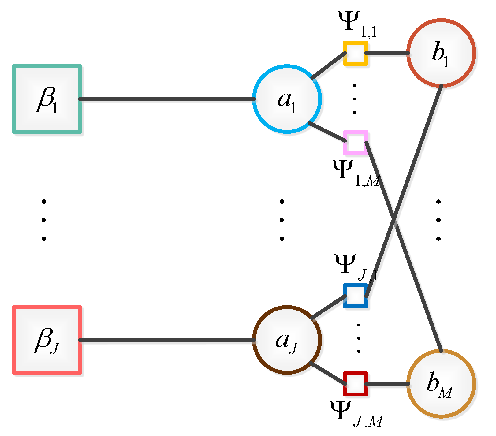
The factorization (23) and (24) can be represented by the factor graph shown in Figure 3. The data association algorithm is done by running belief propagation on the factor graph depicted in Figure 3. Since each factor node is just linked to only two variable nodes, including the target-oriented variable node and the measurement-oriented variable node, an outgoing message from such a factor node is according to
η x j φ q x j = q N j \ q ζ φ q x j x j
where the incoming message from the corresponding variable node is obtained according to
ζ φ q x j x j = φ q x q j N q \ j η x j φ q x j d x j
By further replacing the integral operator by the sum operator, we obtain the messages passed from factor Ψ l , m to target-oriented variable node a k and measurement-oriented variable node b k , respectively, with Equations (28) and (29):
ζ i Ψ l , m b k m b k m = a k l = 1 M k β k l , a k l Ψ l , m a k l , b k m m = 1 m m M k v i 1 Ψ l , m a k l a k l
and
v i Ψ l , m a k l a k l = b k m 0 L k Ψ l , m a k l , b k l l L k \ l ζ i Ψ l , m b k m b k m
for l L k and m 1 , 2 , , M k . The vector-valued message (25) and (26) can be simplified to scalar ones. Due to the admissibility constraint Ψ l , m a k l , b k m each message comprises only two different values. In fact, for ζ i Ψ l , m b k m b k m we get
ζ i Ψ l , m b k m b k m = ζ l , m , b k m = l ζ l , m , b k m l
where
ζ l , m = β k l , m m = 1 m m M k v i 1 Ψ l , m a k l m
and
ζ l , m = a k l = 1 a k l m M k β k l , a k l v i 1 Ψ l , m a k l a k l
Since we are free to normalize message, we define ζ i Ψ l , m b k m b k m as the quotient of Equations (31) and (32) which leads to
ζ i Ψ l , m b k m l = ζ l , m / ζ l , m
and ζ i Ψ l , m b k m b k m = 1 for b k m l . Similarly, we can define the normalized message v i Ψ l , m a k l a k l as
v i Ψ l , m a k l m = v l , m / v l , m
where
v l , m = l L k \ l ζ i Ψ l , m b k m l
and
v l , m = b k m 0 L k b k m l l L k \ l ζ i Ψ l , m b k m b k m
with v i Ψ l , m a k l a k l = 1 for a k l m .
Next, we define the message ζ ¯ i Ψ l , m b k m b k m as the quotient of the quantities ζ ¯ l , m and ζ ¯ l , m , where both quantities are defined equally as ζ l , m and ζ l , m except that v i 1 Ψ l , m a k l m is replaced by their normalized version v i 1 Ψ l , m a k l m . Furthermore, using the fact that all but v i 1 Ψ l , m a k l m = 1 for m = m , the message ζ ¯ i Ψ l , m b k m b k m simplifies to
ζ ¯ i Ψ l , m b k m l = β k l , m β k l , 1 + β k l , 0 + m = 1 m m M k β k l , m v i 1 Ψ l , m a k l m
and ζ ¯ i Ψ l , m b k m b k m = 1 for b k m l . An analogous approach results in the message
v ¯ i Ψ l , m a k l m = 1 1 + l L k \ l ζ k i l m l
and v ¯ i Ψ l , m a k l a k l = 1 for a k l m . Since both message ζ ¯ i Ψ l , m b k m b k m and v ¯ i Ψ l , m a k l a k l just consist of one value that is different from one, we define the scalar-value message ζ k i l m and v k i m l which contain the same information than the vector-valued messages (28) and (29).
As a result, the approximations of both the marginal association probability densities p a k l and p b k l can be obtained via iterative message passing method based on belief propagation. In each belief propagation iteration j 1 , 2 , , J , a message ζ k j l m is passed from variable node a k l via factor node Ψ l , m a k l , b k m to variable node b k m . A message v k j m l is passed from variable node b k m via factor node Ψ l , m a k l , b k m to variable node a k l . According to the principle based on belief propagation and outgoing messages (37) and (38), we can conclude these messages with
ζ k j l m = β k l , m β k l , 1 + β k l , 0 + m = 1 m m β k l , m v k j 1 m l
v k j m l = 1 1 + l L k \ l ζ k j l m
The above recursion established by these two formulations is initialized by v k 0 m l = 1 . Until the final iteration j = J , the approximations of the marginal association probability density p a k l , l L k are obtained by the beliefs at the respective variable nodes a k l . These beliefs are provided by
p a k l = m = { β k l , m / D k l m 1 , 0 β k l , m v k J m l / D k l m 1 , , M k
where the denominator D k l β k l , 1 + β k l , 0 + m = 1 M k β k l , m v k J m l . Similarly, an approximation of p b k m = 0 is obtained as
p ^ b k m = 0 = 1 1 + l L k ζ k J l m
The proposed approximation of the GLMB filtering density is finally obtained by the calculation of the using the belief propagation algorithm. Thus, we conclude that it is an GLMB-form probability density with existence probabilities
r k l = 1 p a k l = 1 = a k l = 0 M k p a k l
and spatial probability density
s l x k = 1 r k l a k l = 0 M k p a k l s l , a k l x k
According to (21), the mixture filtering density is converted to GLMB posterior by the product of its marginals. The posterior density of the GLMB form is given by
π X k = Δ X k L F L θ Θ L w k L , θ δ L L X p ^ k L , θ X
where
w k L , θ l L \ L 1 r k l l L r k l η l , θ
p ^ L , θ = s l x k
The multi-target states are estimated using the posterior density π X k in (45). As discussed above, a pseudocode of the GLMB-TBD filter based on belief propagation is depicted in Algorithm 1.
Algorithm 1: The GLMB-TBD filter based on belief propagation algorithm
Input: The initial birth density of the LMB form at time k = 0 : r 0 l , p l x 0 l B
Output: The multi-target tracks l L k for each time
For l L k do
 Calculate β k l , m for m 0 , 1 , , M k as β k l , m = r k | k 1 l η l , m with η l , m given in
 (18) and for m = 1 as β k l , 1 = 1 r k | k 1 l , respectively
 Calculate the spatial probability density s l , m x k for m 0 , 1 , , M k
 according to (19)
End for
Initialize v k 0 m l = 1 For j = 1 : J do
 Calculate ζ k j l m according to (39)
 Calculate v k j m l according to (40)
End for
Calculate the approximate marginal association probabilities p ^ a k l and p ^ b k m = 0
according to (41) and (42), respectively
Calculate the update existence probabilities r k l and spatial probability densities
s l x k for l L k according to (43) and (44), respectively
Calculate the GLMB posterior density according to (46) and (47)
Estimate the cardinality distribution and multi-target state using the maximum a posterior method

3.2. Complexity Analysis

In this section, we give the complexity analysis of the proposed BP-based version and compare it with the state-of-the-art algorithms. The complexity of the deterministic solution such as Murty algorithm in [11] is O N M + 2 P 4 , i.e., biquadrate in the number of both Bernoulli components and measurements. More efficient deterministic algorithms can reduce the complexity to O N M + 2 P 3 , i.e., cubic at best in the number of both Bernoulli components and measurements. A much cheaper and simpler algorithm based on Gibbs sampling in [25] is presented with the complexity O N P 2 M is the number of Gibbs samples in random sampler, P and M denote the numbers of Bernoulli components and measurements, respectively. That is to say, the complexity of the Gibbs-based version is quadratic in the number of Bernoulli components and linear in the number of measurements. By contrast, the complexity of the BP-based GLMB-TBD filter is caused by the belief propagation iteration operation with linear in number of the iteration J . Therefore, the complexity of the proposed algorithm is O J P M , where J denotes the belief propagation time. The message in BP-based algorithm is passed iteratively to implement the GLMB-TBD filter instead of sampling over the posterior density. Hence, the sampler N is replaced by iteration J . In order to balance the tracking performance between estimate precision and computational complexity, a typical value of iteration J is set to be 20. For clarity, the computational complexity of the tested algorithms is summarized in Table 1.

4. Results

In this section, the performance of the proposed algorithm is verified via the following simulation experiments. Throughout this section, each track in our recursive multi-target tracker is implemented with a particle filter approximation due to non-linear measurement model. Details of the particle implementation of the GLMB-TBD based on belief propagation is given in references [11,19].
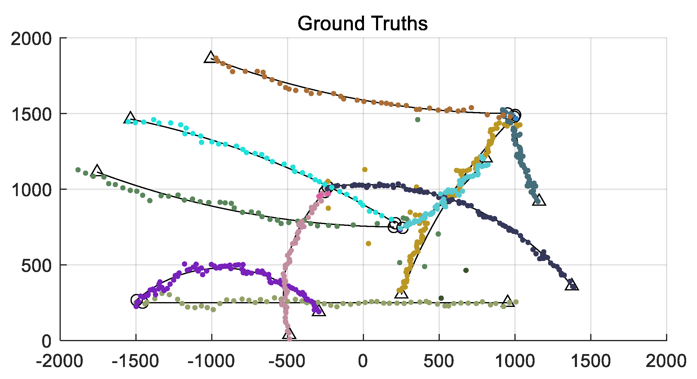
To assess the performance of the proposed GLMB-TBD filter based on belief propagation with particle filter implementation, we adopt it to track up to ten targets in the challenging multi-target tracking scenario over a surveillance region 2000 , 2000 m × 0 , 2000 m , as shown in Figure 4. The target state x k = x ˜ k T , ω k , a ζ T , where x ˜ k = p x , k , p ˙ x , k , p y , k , p ˙ y , k T is the position and velocity vector and ω k is the turn rate and a ζ is amplitude fluctuation. The targets evolve according to the coordinate turn model with an i.i.d. Gaussian driving process of variance σ u . The transition density for the coordinated turn model is given by f k | k 1 x k | x k 1 = N x k ; m x k 1 , Q , where m x k 1 = F ω k x ˜ k T , ω k T , Q = diag σ ω 2 G G T , σ u 2 , a ζ T s with σ ω = 15 m / s 2 , σ u = π / 180 rad / s ,
F ω = 1 sin ω T s ω 0 1 cos ω T s ω 0 cos ω T s 0 sin ω T s 0 1 cos ω T s ω 1 sin ω T s ω 0 sin ω T s 0 cos ω T s   and   G = T s 2 2 0 T s 0 0 T s 2 2 0 T s
where T s , a ζ denote the radar sampling interval and amplitude fluctuation, respectively. The state independent survival probability of the targets is given by p S = 0.99 . The new-birth target follows a multi-Bernoulli RFS with density parameter π B = r B i , s B i i = 1 4 , where r B 1 = r B 2 = 0.03 , r B 3 = r B 4 = 0.04 , s B i x = N x ; m B i , P B .
In the following numerical simulations, to set the different low SNR values for the challenging scenario with multi-target tracking, let S N R be signal-to-noise ratio defined in dB as
S N R = 10 log A ¯ 2 2 σ n 2
where A ¯ denotes the amplitude of the complex echo of the target, and σ n 2 denotes the Gaussian noise variance. The estimated tracks and true tracks for x-y plane is shown in Figure 5. It is seen that the proposed algorithm achieves satisfied performance.
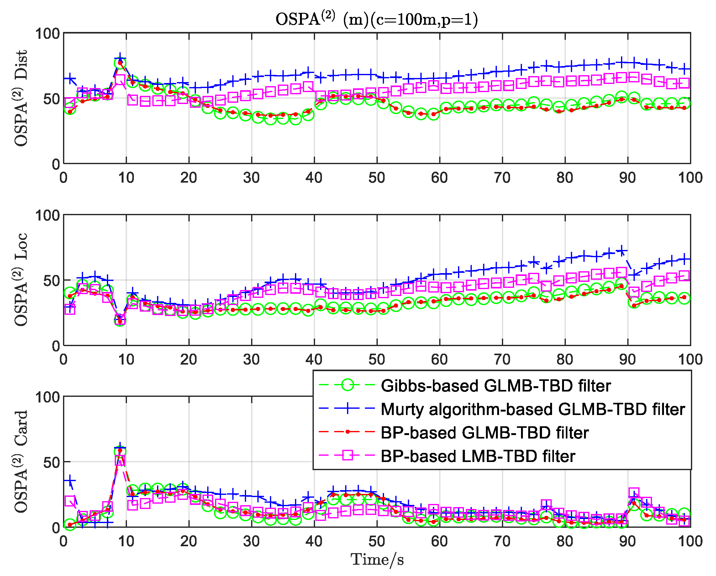
In a radar TBD scenario under the non-separable likelihood assumption, the clutter measurements are uniformly distributed on the observation space and is a Poisson RFS with κ k z = λ c V U z , where U denotes a uniform density on the observation region. The effective target template C x is set to be 3 pixel × 3 pixel square region whose center is closest to the position of x . The optimal sub-pattern assignment ( OSPA 2 ) metric with a physically meaningful base-distance is adopted to construct a physically meaningful distance between two sets of tracks. Furthermore, the OSPA 2 with window length L w = 10 is used to provide an indication of the multi-target tracking performance [26]. The other relevant parameters used in the numerical simulations are reported in Table 2.
To demonstrate the scalability of the proposed BP-based implementation of GLMB-TBD filter, the performance in both estimation accuracy and computational complexity is compared to three implementations: Murty algorithm-based implementations, Gibbs sampling-based implemenation and the Belief propagation-based implementation. The LMB-TBD filter based on BP implementation is compared to demonstrate the superior tracking performance of the BP-based GLMB-TBD filter.
It can be shown in Figure 6 that the tracking accuracy of the BP-based version is better than that of the Gibbs-based version due to preserving the relevant association information, which is pruned by the Gibbs sampling. The implementation based on Gibbs sample is performed by truncating GLMB components resulting in accuracy loss. However, that issue does not exist in the BP-based implementation. Using the belief propagation algorithm, the GLMB-TBD filter significantly outperforms the LMB-TBD filter in tracking accuracy since the GLMB RFS is the exact closed-form solution to Bayesian inference. Additionally, the tracking precision of the Murty-based version degrades less than that of both BP-based version and Gibbs-based version due to discarding insignificant hypotheses.
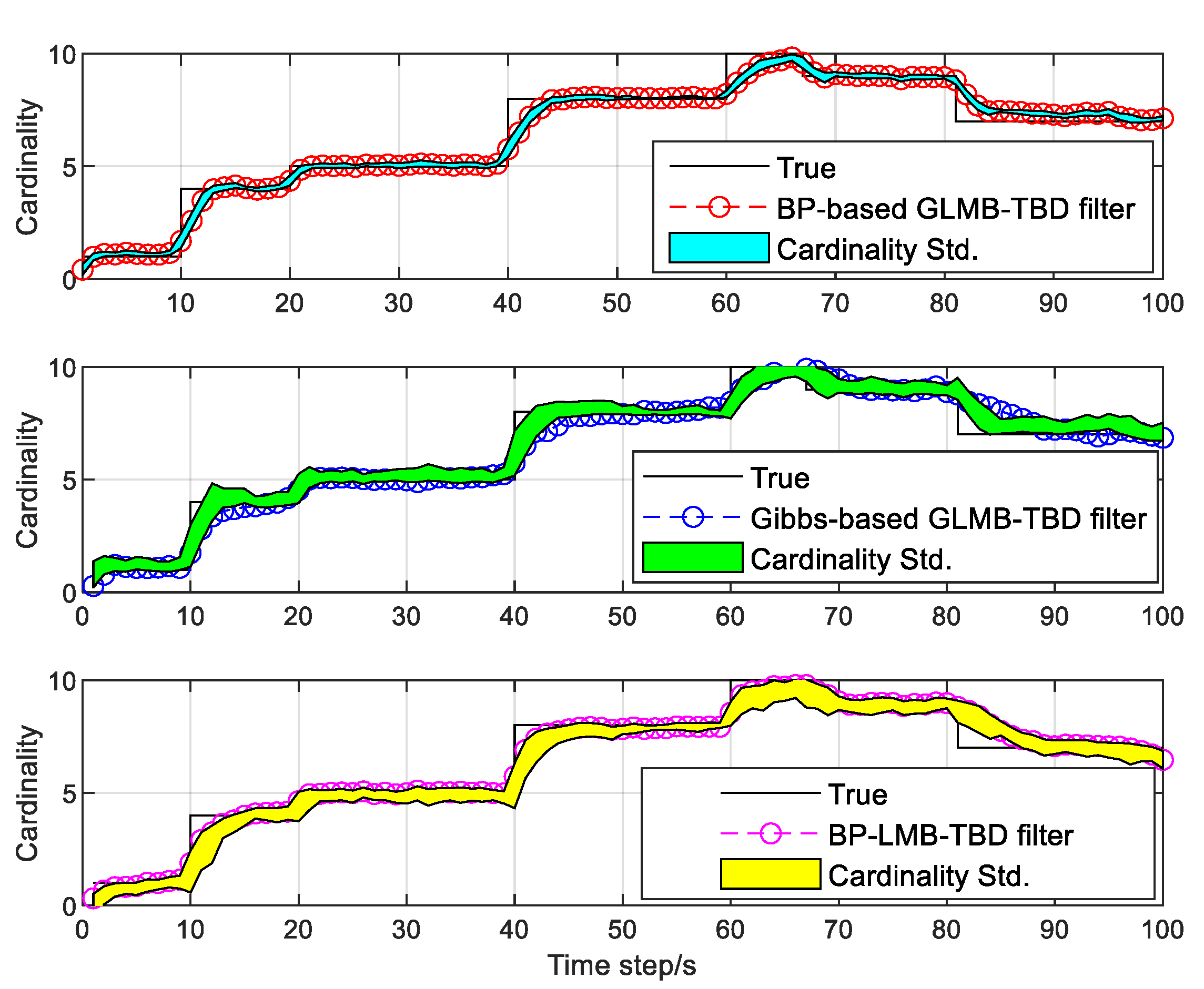
Figure 7 shows the mean and standard deviation of the estimated cardinality versus time. For the cardinality estimation, BP-based version is obviously better than the Gibbs-based version. With the BP-based implementation, the GLMB-TBD filter is better than the LMB-TBD filter in the cardinality estimate.
Figure 8 plots the computational cost of the different methods. The GLMB-TBD filter based on the Murty algorithm has high computational complexity due to complex high-dimensional data association map and at best cubic complexity in the number of measurements. The results for the runtimes show that the GLMB-TBD filter based BP is less complex than the Gibbs-based version due to liner complexity in the number of the Bernoulli component in posterior density. The BP-based LMB-TBD filter can slightly reduce the computational complexity compared to BP-based GLMB-TBD filter, whereas it suffers from performance degradation in tracking precision.
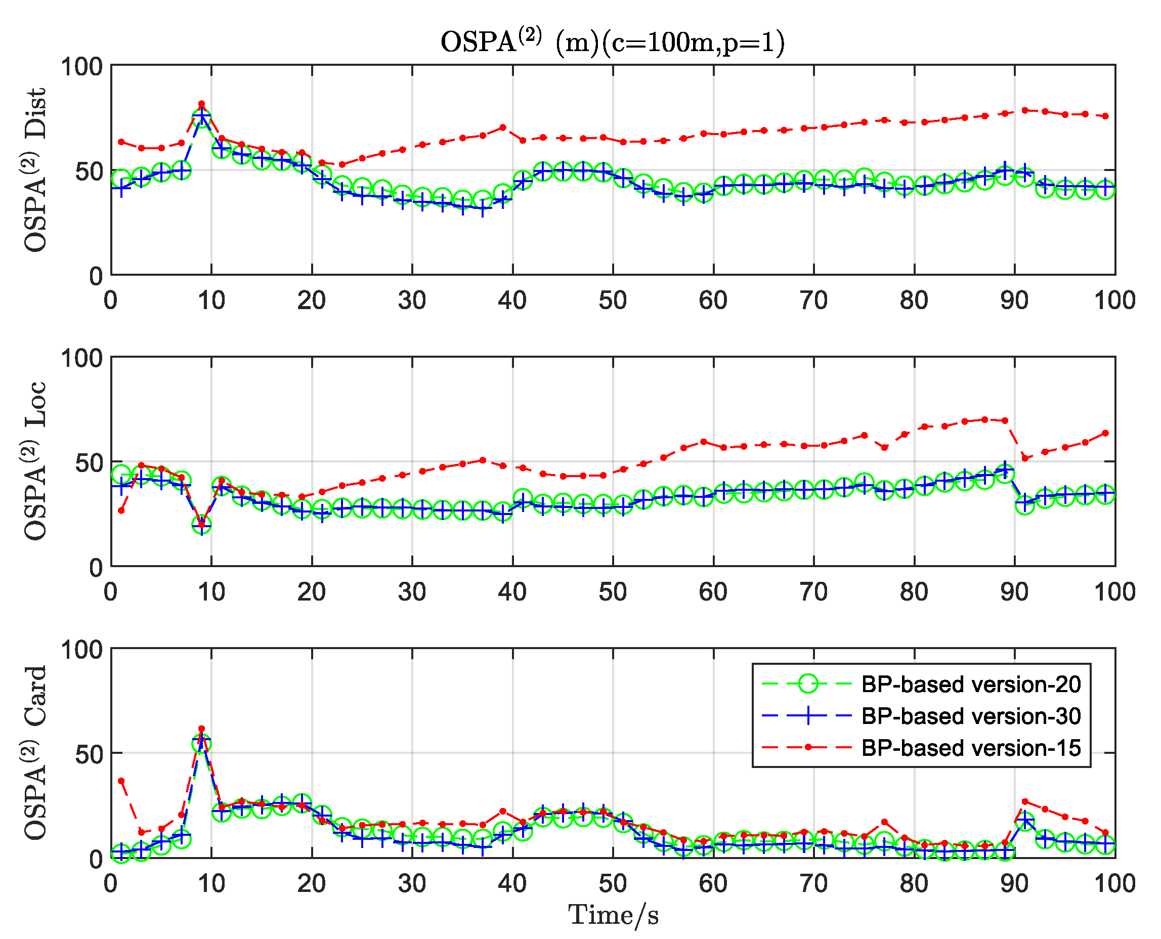
It is observed in Figure 9 that the tracking performance of the proposed BP-version is better with the more iterative time. However, the OSPA error does not decrease more when the iterative time reaches a certain degree.
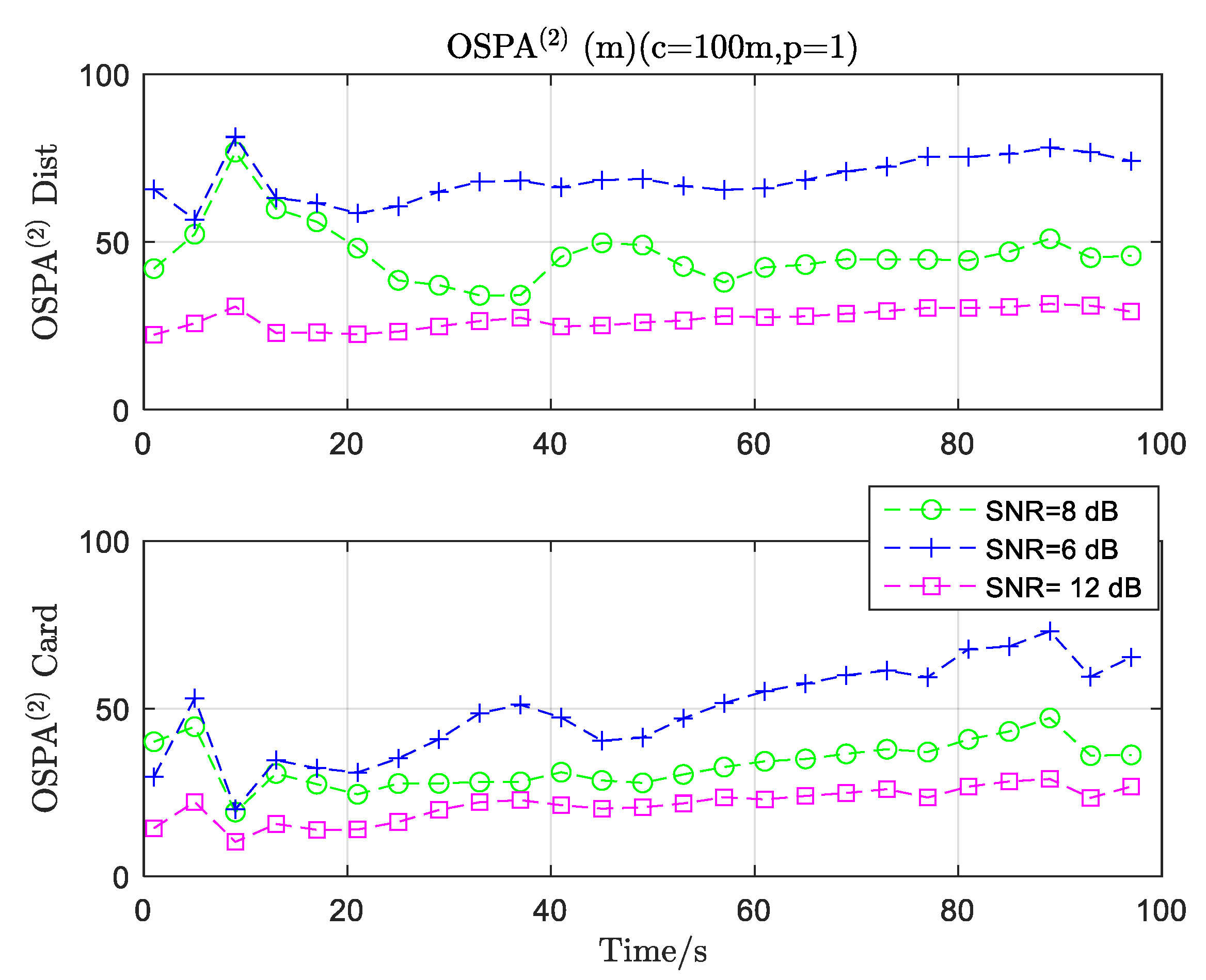
According to (48), the simulation experiment is set by different low-SNR values. It is shown in Figure 10 that the proposed algorithm can effectively implement the tracking of multiple weak targets in challenging scenarios with low SNR.

5. Discussion

The GLMB filter with TBD measurement model based on BP algorithm is proposed for tracking multiple weak targets. Using the belief propagation algorithm, the mixture density output by the GLMB-TBD filter is translated into posterior density of GLMB form for recursively estimating multi-target states. Contrary to the Gibbs sampling-version, the proposed BP-version is superior in tracking performance. On one hand, the estimate accuracy of BP-version is better than that of Gibbs sampling-version due to the preservation of relevant association information. On the other hand, the computational cost of the BP-version is less than that of the Gibbs sampling-based version due to linear complexity in the number of the Bernoulli component. Compared with the KLD-based implementation, the BP-based version can effectively calculate the marginal densities with reduced complexity. The GLMB-TBD filter based on the BP algorithm is a promising approach for tracking multiple weak targets. While single-sensor systems are sometimes sufficient, a multiple-sensor framework is required to reduce uncertainty on the number of targets along with their states, yielding improved multi-target tracking performance. A venue for further research is the generalization of the proposed method to multiple-sensor scenario.

6. Conclusions

The GLMB filter based on the TBD measurement model is not the same type as the prior density due to closure loss. The implementation based on KLD is faced with a large computational load. In this paper, the belief propagation algorithm is used for accommodating the multi-target posterior recursion via approximately calculating the marginal association probabilities. Thus, the BP-based version of GLMB-TBD filter is formulated to track multiple weak targets. Specifically, the BP-based GLMB-TBD filter possesses better estimate precision than Gibbs-based version due to preserving the relevant association information in the update step. More importantly, the BP-based implementation of the GLMB-TBD filter has linear complexity in the number of the Bernoulli component and measurement. The simulation results demonstrate that the proposed algorithm can computationally, efficiently track multiple weak targets.
In the Bayesian estimation for state-space models, smoothing yields significantly better estimates than filtering by using the history of the states rather than the most recent state [27,28]. In addition, multi-sensor tracker generally benefits from larger detection range and immunity to single-sensor faults. Thus, a venue for further research is the generalization of the proposed technique to multi-frame version of the GLMB model and multi-sensor version of the GLMB filter [29,30,31,32]. On the other hand, the Gaussian BP algorithm is an effective method for multi-target tracking of multiple sensors. Hence, the extension of the proposed BP algorithm to the Gaussian version is another further work for solving weak target tracking of the multiple sensors. More importantly, the convergence of the belief propagation is crucial to the performance of the tracking algorithm based on the proposed algorithm. The convergence discussion is, however, out of the scope of this paper. Hence, the convergence analysis of the belief propagation will be another research subject.

Author Contributions

C.C. conceived the idea and developed the proposed methods. C.C. wrote the original draft. Y.Z. advised the research and helped edit the paper. Y.Z. worked on project administration, supervision, and funding acquisition. All authors have read and agreed to the published version of the manuscript.

Funding

Foreign Scholars in University Research and Teaching Programs (the 111 Project) (No. B18039).

Acknowledgments

The authors would like to thank the reviewers for their valuable suggestions on improving this paper.

Conflicts of Interest

The authors declare no conflict of interest.

References

  1. Zhu, Y.; Wang, J.; Liang, S. Efficient joint probabilistic data association filter based on Kullback-Leibler divergence for multi-target tracking. IET Radar Sonar Navig. 2017, 11, 1540–1548. [Google Scholar] [CrossRef]
  2. Blackman, S.S. Multiple hypothesis tracking for multiple target tracking. IEEE Trans. Aerosp. Electron. Syst. 2004, 19, 5–18. [Google Scholar] [CrossRef]
  3. Li, C.; Wang, W.; Kirubarajan, T.; Sun, J.; Lei, P. PHD and CPHD filtering with unknown detection probability. IEEE Trans. Signal Process. 2018, 66, 3784–3798. [Google Scholar] [CrossRef]
  4. Vo, B.-T.; Vo, B.-N.; Cantoni, A. Analytic implementations of the cardinalized probability hypothesis density filter. IEEE Trans. Signal Process. 2007, 55, 3553–3567. [Google Scholar] [CrossRef]
  5. Jones, B.A. CPHD filter birth modeling using the probabilistic admissible region. IEEE Trans. Aerosp. Electron. Syst. 2018, 54, 1456–1469. [Google Scholar] [CrossRef]
  6. Mahler, R.P.S.; Vo, B.-T.; Vo, B.-N. CPHD filter with unknown clutter rate and detection profile. IEEE Trans. Signal Process. 2011, 59, 3497–3513. [Google Scholar] [CrossRef]
  7. Bryant, D.S.; Delande, E.D.; Gehly, S.; Houssineau, J.; Clark, D.E.; Jones, B.A. The CPHD filter with target spawning. IEEE Trans. Signal Process. 2017, 65, 13124–13138. [Google Scholar] [CrossRef]
  8. Nguyen, T.T.D.; Vo, B.-N.; Vo, B.-T.; Kim, D.Y.; Choi, Y.S. Tracking Cells and Their Lineages Via Labeled Random Finite Sets. IEEE Trans. Signal Process. 2021, 69, 5611–5626. [Google Scholar] [CrossRef]
  9. Vo, B.-T.; Vo, B.-N. Labeled Random Finite Sets and Multi-Objects Conjugate Priors. IEEE Trans. Signal Process. 2013, 61, 3460–3475. [Google Scholar] [CrossRef]
  10. Bryant, D.S.; Vo, B.-T.; Vo, B.-N.; Jones, B.A. A generalized labeled multi-Bernoulli filter with object spawning. IEEE Trans. Signal Process. 2018, 66, 6177–6189. [Google Scholar] [CrossRef] [Green Version]
  11. Vo, B.-N.; Vo, B.-T.; Phung, D. Labeled random finite sets and the Bayes multi-target tracking filter. IEEE Trans. Signal Process. 2014, 62, 6554–6567. [Google Scholar] [CrossRef]
  12. Reuter, S.; Vo, B.-T.; Vo, B.-N.; Dietmayer, K. The labeled multi-Bernoulli filter. IEEE Trans. Signal Process. 2014, 62, 3246–3260. [Google Scholar]
  13. Yi, W.; Jiang, M.; Hoseinnezhad, R. The multiple model Vo-Vo filter. IEEE Trans. Aerosp. Electron. Syst. 2017, 53, 1045–1054. [Google Scholar] [CrossRef]
  14. Punchihewa, Y.G.; Vo, B.-T.; Vo, B.-N.; Kim, D.Y. Multiple object tracking in unknown backgrounds with labeled random finite sets. IEEE Trans. Signal Process. 2018, 66, 3040–3055. [Google Scholar] [CrossRef]
  15. Vo, B.-N.; Vo, B.-T.; Pham, N.-T.; Suter, D. Joint detection and estimation of multiple objects from image observations. IEEE Trans. Signal Process. 2010, 58, 5129–5141. [Google Scholar] [CrossRef]
  16. Chai, L.; Kong, L.; Li, S.; Yi, W. The multiple model multi-Bernoulli filter based track-before-detect using a likelihood based adaptive birth distribution. Signal Process. 2020, 171, 1–11. [Google Scholar] [CrossRef]
  17. Papi, F.; Vo, B.-N.; Vo, B.-T.; Fantacci, C.; Beard, M. Generalized Labeled Multi-Bernoulli Approximation of Multi-Object Densities. IEEE Trans. Signal Process. 2015, 63, 5487–5497. [Google Scholar] [CrossRef]
  18. Li, S.; Yi, W.; Hoseinnezhad, R.; Wang, B.; Kong, L. Multi-object Tracking for Generic Observation Model Using Labeled Random Finite Sets. IEEE Trans. Signal Process. 2018, 66, 368–383. [Google Scholar] [CrossRef]
  19. Papi, F.; Kin, D.T. A Particle Multi-Target Tracker for Superpositional Measurements Using Labeled Random Finite Sets. IEEE Trans. Signal Process. 2015, 63, 4348–4358. [Google Scholar] [CrossRef]
  20. Cao, C.; Zhao, Y. An efficient implementation of the multiple-model generalized labeled multi-Bernoulli filter for track-before-detect of point targets using an image sensor. IEEE Trans. Aerosp. Electron. Syst. 2021, 57(6), 4416–4432. [Google Scholar] [CrossRef]
  21. Yi, W.; Fang, Z.; Li, W.; Hoseinnezhad, R.; Kong, L. Multi-Frame Track-Before-Detect Algorithm for Maneuvering Target Tracking. IEEE Trans. Veh. Technol. 2020, 69, 4104–4118. [Google Scholar] [CrossRef]
  22. Williams, J.; Lau, R. Approximate evaluation of marginal association probabilities with belief propagation. IEEE Trans. Aerosp. Electron. Syst. 2014, 50, 2942–2959. [Google Scholar] [CrossRef]
  23. Kropfreiter, T.; Meyer, F.; Hlawatsch, F. A fast labeled multi-Bernoulli using belief propagation. IEEE Trans. Aerosp. Electron. Syst. 2020, 56, 2478–2488. [Google Scholar] [CrossRef]
  24. Soldi, G.; Meyer, F.; Braca, P.; Hlawatsch, F. Self-tuning algorithm for multisensor-multitarget tracking using belief propagation. IEEE Trans. Signal Process. 2019, 67, 3922–3937. [Google Scholar] [CrossRef]
  25. Vo, B.-N.; Vo, B.-T.; Hoang, H.G. An Efficient Implementation of the Generalized Labeled Multi-Bernoulli Filter. IEEE Trans. Signal Process. 2017, 65, 1975–1987. [Google Scholar] [CrossRef]
  26. Beard, M.; Vo, B.-T.; Vo, B.-N. Bayesian multi-target tracking with merged measurements using labeled random finite sets. IEEE Trans. Signal Process. 2015, 63, 1433–1447. [Google Scholar] [CrossRef]
  27. Beard, M.; Vo, B.-T.; Vo, B.-N. A solution for large-scale multi-object tracking. IEEE Trans. Signal Process. 2020, 68, 2754–2769. [Google Scholar] [CrossRef]
  28. Vo, B.-N.; Vo, B.-T. A multi-scan labeled random finite set model for multi-object state estimation. IEEE Trans. Signal Process. 2019, 67, 4948–4963. [Google Scholar] [CrossRef]
  29. Vo, B.-N.; Vo, B.-T.; Beard, M. Multi-sensor multi-object tracking with the generalized labeled multi-Bernoulli filter. IEEE Trans. Signal Process. 2019, 67, 5952–5967. [Google Scholar] [CrossRef]
  30. Yi, W.; Chai, L. Heterogeneous multi-sensor fusion with random finite set multi-object densities. IEEE Trans. Signal Process. 2021, 69, 3399–3414. [Google Scholar] [CrossRef]
  31. Wang, B.; Li, S.; Battistelli, G. Multi-agent fusion with different limited-fields-of-view. IEEE Trans. Signal Process. 2022, 70, 1560–1575. [Google Scholar] [CrossRef]
  32. Nguyen, H.V.; Rezatofighi, H.; Vo, B.-N.; Ranasinghe, D.C. Distributed multi-object tracking under limited field of view sensors. IEEE Trans. Signal Process. 2021, 69, 5329–5344. [Google Scholar] [CrossRef]
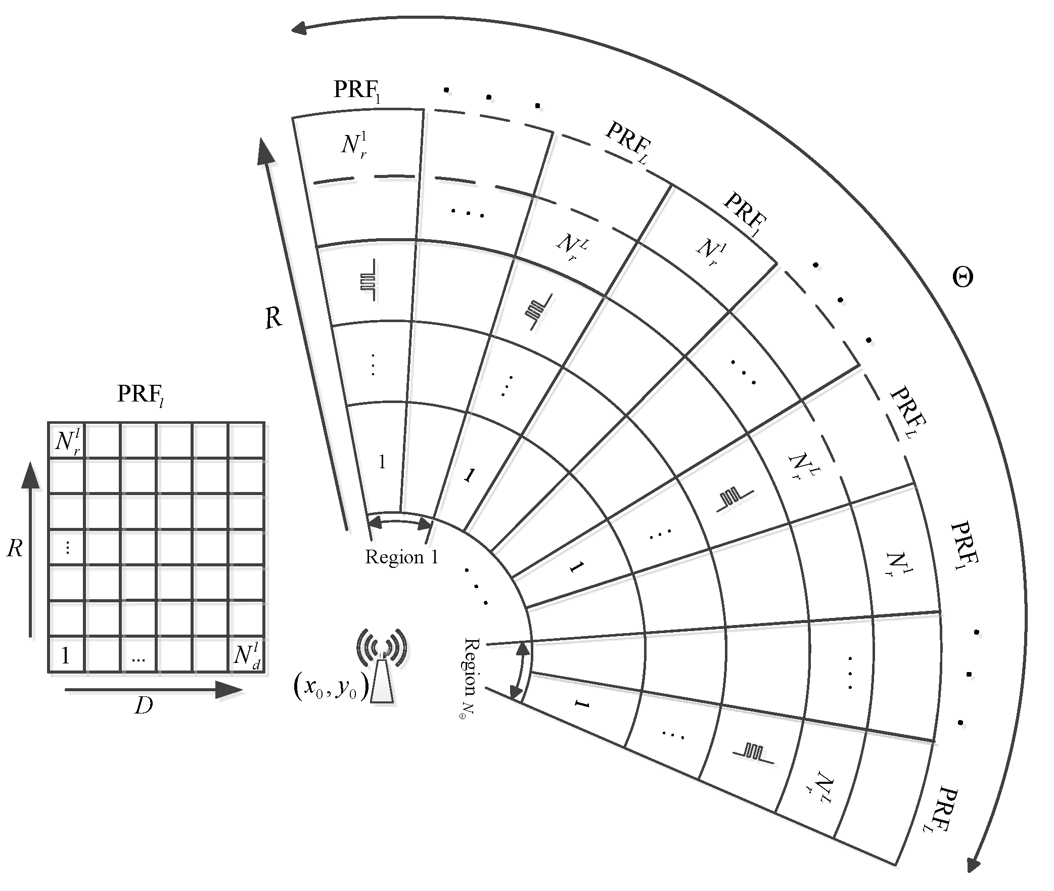
Figure 1. The radar surveillance region in the radial range, angle, and Doppler dimensions.
Remotesensing 14 04209 g001
Figure 2. The illustrated template in an image pixeled TBD measurement model.
Remotesensing 14 04209 g002
Figure 3. Factor graph representing the factorization (20) and (21).
Remotesensing 14 04209 g003
Figure 4. Multiple-target trajectories in the x y plane. Start/Stop positions for each track are shown with ○/△. And different colored lines represent different trajectories.
Remotesensing 14 04209 g004
Figure 5. The estimated track of multiple targets for a single MC run. The colored dots represent the estimated position.
Remotesensing 14 04209 g005
Figure 6. The error curves for the final estimations from the different methods over 100 Monte Carlo runs.
Remotesensing 14 04209 g006
Figure 7. Cardinality statistics for the different methods over 100 Monte Carlo trials.
Remotesensing 14 04209 g007
Figure 8. The execution-time curves versus time for different tracking methods.
Remotesensing 14 04209 g008
Figure 9. The OSPA(2) error of the BP-version for different iterative time.
Remotesensing 14 04209 g009
Figure 10. The error curves of the proposed algorithm for different SNRs.
Remotesensing 14 04209 g010
Table 1. The complexity of the tested algorithms.
Tested AlgorithmComplexity
Murty algorithm-based version O N M + 2 P 4
Gibbs-based version O N P 2 M
BP-based version O J P M
Table 2. The main parameters of the simulation.
ParameterSymbolValue
Sampling period T s T s = 1   s
Iterative time J J = 20
Loss coefficient L r , L d , L θ L r = L d = L θ = 1
Amplitude fluctuation a ζ a ζ = 1
Signa-to-noise ratioSNR7 dB
1st Birth target state x B 1 x B 1 = 1500 , 0 , 250 , 0 , 0 T
2nd Birth target state x B 2 x B 2 = 250 , 0 , 1000 , 0 , 0 T
3rd Birth target state x B 3 x B 3 = 250 , 0 , 750 , 0 , 0 T
4th Birth target state x B 4 x B 4 = 1000 , 0 , 1500 , 0 , 0 T
Birth covariance Q B Q B = diag 50 , 50 , 50 , 50 , 8 π / 180 2
Publisher’s Note: MDPI stays neutral with regard to jurisdictional claims in published maps and institutional affiliations.