Article

A Deep Learning Application to Map Weed Spatial Extent from Unmanned Aerial Vehicles Imagery

1
IBM Research Europe, Daresbury WA4 4AD, UK
2
Department of Animal and Plant Sciences, University of Sheffield, Sheffield S10 2TN, UK
3
Rothamsted Research, Harpenden AL5 2JQ, UK
*
Author to whom correspondence should be addressed.
Remote Sens. 2022, 14(17), 4197; https://doi.org/10.3390/rs14174197
Submission received: 18 July 2022 / Revised: 10 August 2022 / Accepted: 17 August 2022 / Published: 26 August 2022
(This article belongs to the Special Issue Deep Learning for Remote Sensing Image Classification II)

Abstract

:
Weed infestation is a global threat to agricultural productivity, leading to low yields and financial losses. Weed detection, based on applying machine learning to imagery collected by Unmanned Aerial Vehicles (UAV) has shown potential in the past; however, validation on large data-sets (e.g., across a wide number of different fields) remains lacking, with few solutions actually made operational. Here, we demonstrate the feasibility of automatically detecting weeds in winter wheat fields based on deep learning methods applied to UAV data at scale. Focusing on black-grass (the most pernicious weed across northwest Europe), we show high performance (i.e., accuracy above 0.9) and highly statistically significant correlation (i.e., ro > 0.75 and p < 0.00001) between imagery-derived local and global weed maps and out-of-bag field survey data, collected by experts over 31 fields (205 hectares) in the UK. We demonstrate how the developed deep learning model can be made available via an easy-to-use docker container, with results accessible through an interactive dashboard. Using this approach, clickable weed maps can be created and deployed rapidly, allowing the user to explore actual model predictions for each field. This shows the potential for this approach to be used operationally and influence agronomic decision-making in the real world.

Graphical Abstract

1. Introduction

Weeds are responsible for the greatest potential yield losses in agricultural production, making control of weeds of considerable importance to growers [1]. Weed control measures are also associated with significant costs, both financially, and in terms of time taken to implement control [2]. Weed surveillance is therefore an important primary step in controlling weeds, to ensure that the weed management tactics employed are appropriate, and commensurate with the severity of the weed infestation. Accurate weed surveillance is a necessity for more targeted, precision weed management, such as variable rate or site-specific herbicide application. This can lower the cost of effective weed control for the grower, whilst providing additional environmental benefits including reductions in the area and total volume of herbicide application [3,4]. In order to facilitate a proportionate and effective weed control strategy, it is therefore important to have an accurate understanding of the spatial extent and abundance of the target weed species.
Accurate and timely weed surveillance is challenging due to the difficulties in collecting sufficient, good quality weed abundance data over large areas [5,6]. Nevertheless, the rapid proliferation in recent years of relatively low-cost, camera-equipped Unmanned Aerial Vehicles (UAVs), has made the collection of high-resolution RGB, multi- and hyper-spectral imagery of crop fields easier and more affordable. In tandem with this, advances in Artificial Intelligence through machine and deep learning approaches are revolutionising our capacity to derive both qualitative and quantitative data from imagery. Specifically, over the last decade there has been a proliferation of deep learning computer vision studies (n = 426) focused on Earth Observation (e.g., using UAV or satellite images) [7], with a number of state-of-the-art architectural approaches that have been successfully adopted across a range of domains (e.g., settlements and transportation mapping as well as agriculture). Particularly, as reported by Hoeser et al. [7], different forms of ResNet and VGG architectures were the most popular choice among convolutional backbones to extract relevant features (35% and 25%, respectively), while Encoder–Decoder architectures were the most used for image segmentation tasks (62%). In this group, UNET was the preferred choice (33%) followed by Patch Based approaches (26%), Fully Convolutional Networks (15%) and SegNet (17%) [7].
Given these technical advancements, the application of UAV-derived imagery and subsequent weed recognition has received considerable attention in recent years as a means for rapid, remote detection of weeds [8,9,10], with some studies showing promising results in generating accurate weed maps [11,12,13,14,15,16,17] and for tailoring subsequent precision weed management [18,19,20,21]. Despite this promise, actual uptake of remote weed detection for field agronomy has remained limited, and several challenges remain before this technology receives wider adoption [22]. Whilst use of unmanned systems makes the collection of data more rapid, there remain issues caused by the sheer size of the generated imagery files; both in terms of its storage, and the computing resources needed for orthomosaicing, data labelling, and analysis [23]. Often this can lead to considerable time between the collection of data and its subsequent processing into a usable form [24]. Furthermore, while mapping in certain crop–weed combinations—such as in wide-row crops or grasses in broad-leaved crops and vice versa, have been relatively successful (e.g., [18,25,26]), other situations are intrinsically more difficult for classification. Detection of grassweed species in cereals remains taxing; as both crop and weed are grasses, their morphological and spectral properties are frequently very similar, and narrow-row cereal cropping situations lead to considerable overlap and masking between plants [22,27].
To date, a considerable portion of remote weed mapping studies have focused on surveillance of relatively small areas, or small experimental plots with contrasting weed abundance [28]. This often leads to good classification performance, but raises questions on the generalisability of the results and performance of models when applied to other fields. Small differences in weather, crop/weed phenology, and crop variety at the time of imaging could have a considerable impact on the performance of classifiers. Indeed, studies which have included a true test of out-of-bag performance generally reported much reduced accuracy [12,13], highlighting the difficulty in creating robust, generalisable predictions. Similarly, it has been highlighted that the vast majority of published studies (i.e., 85%) are solely reliant on post-hoc annotation of images for both weed discrimination and assessment of performance, with far fewer studies (i.e., less than 8%) making use of actual field observations [10], while there are practical considerations that underpin this, relating machine learning derived weed maps to actual field observations remains an important step in both verifying model accuracy, and ensuring the perceived reliability of results to support their wider use within the agricultural and research communities.
In this study, we present the use of deep learning techniques on UAV-derived RGB and multispectral imagery to discern weed infestations in winter wheat crops at plant maturity in 34 fields within the UK. In particular, we focus on infestations of the weed species black-grass (Alopecurus myosuroides), the UK’s most pernicious weed [29,30], estimated to cost the UK economy GBP 0.4 billion in lost gross profit annually due to wheat yield losses of 0.8 million tonnes [2]. Conversely to previous studies, we present our results on large out of bag data and relate results back to in-field ground-truth data. We demonstrate good concordance between imagery-derived local and global weed maps and the current mapping practice adopted for ecological research of this weed. Finally, we demonstrate how our resulting model can be made operational via a lightweight Docker container, and present a prototype of a dashboard for growers consumption.

2. Methods

2.1. Data Collection

2.1.1. UAV Data

To minimise variability and maximise dataset size for training of deep learning models, we chose to focus on one specific crop type: winter wheat (WW). We collected data for 40 fields across the UK, chosen from an existing black-grass surveillance network. Field sites were chosen based on prior years’ black-grass surveillance data, maximising the likelihood that the selected fields would have appropriate and measurable black-grass infestations.
Flights were undertaken using a DJI M210 UAV, with mounted X7 sensors, which collected RGB data at a 1 cm resolution and multispectral data at 3 cm resolution. This combination of RGB and multispectral imagery was collected as both forms of data have been shown to contribute to crop/weed classification in other studies and systems [11,12,13]. Each field was flown at a speed of 4 m/s and 45 m height between 9 a.m. and 4 p.m. These resolutions and collection procedures were based on optimisation over the previous 2019 and 2020 seasons (data not shown), and represent an optimal compromise between image quality, speed of capture, and file sizes. Orthomosaicing was performed with the Pix4d software, using the default settings. Fields were originally flown in mid-May 2021, and each field’s RGB image was inspected to confirm crop type, crop establishment, and to verify the quality of imagery collected using this protocol. To generate the dataset for analysis, fields were flown again between mid-June and mid-July 2021, when black-grass is most apparent due to its flowering heads above the crop. Fields were not flown in the rain or in high winds (e.g., greater than 10 m/s); however, the resultant imagery over this 4-week period captures other aspects of variability including differences in crop variety, time of day, and weather conditions (e.g., overcast days, sunny days or scattered clouds). This allows the model training and test datasets to include these components, rather than developing a model specific to one field, time-point, or variety. Again, before annotation and analysis, data were visually inspected to ensure that the RGB and multispectral imagery were present and complete, that minimal artefacts following orthomosaicing occurred, and that the captured resolution was correct (1 cm RGB, 3 cm multispectral).

2.1.2. Field Survey Data

To evaluate the relevance and applicability of our results to the real world, field weed abundance data was collected for 31 of the 40 fields flown with UAVs, using a current manual mapping practice adopted for ecological research of black-grass [6]. For each field, a contiguous grid of 20 × 20 m geolocated quadrats was established. Fields were visited at crop/weed maturity within 1–2 weeks of UAV imaging. For each quadrat, the severity of black-grass infestation was estimated by eye on a scale of; 0-absent, 1-low, 2-medium, 3-high, 4-very high (see example in Figure 1). The resultant survey data was used to aid with validation of model predictions during analysis. The total surveyed area included 5132 quadrats (205 hectares), with fields that ranged from 27 (1.1 hectares) to 291 (71.1 hectares) quadrats and an average of 171 quadrats (6.8 hectares).

2.2. Data Processing

2.2.1. Data Labelling

Of the 40 fields for which we collected data, six had to be excluded from analysis due to issues with crop establishment (e.g., re-sowing of an alternative crop species), or technical issues with the imagery such as lack of multispectral data. The RGB image files for the 34 fields included were then uploaded onto the CVAT data labelling software [31]. Due to the large amount, and high resolution, of data to be labelled, a team composed of a weed monitoring expert and three computer scientists was involved in the data labelling. To ensure consistency in the label quality, all members of the data labelling team received training in differentiating between crop and weed from the expert in weed monitoring. During training, it was agreed to target reasonably sized weed patches, rather than individual plants, which would be both difficult to spot and extremely time-consuming to annotate across all imagery. The 34 fields were therefore split equally between the four different team members, with one team member who also checked and confirmed that quality was consistently satisfactory across all fields.
The main caveat with the labels produced in this way is that drawing polygons around patches, rather than trying to draw plant contours precisely, might not be ideal for model training and validation (e.g., background or other plants might be included if in very close proximity to weed patches). However, data labelling at scale for deep learning weed detection is a known issue [17], and in this project we aimed at reaching a compromise to maximise resources and effort in a task that otherwise would have not been feasible at the scale of our dataset.

2.2.2. Dataset Creation

The weed data labels were retrieved from CVAT and weed label file maps were created for each field. At this point original RGB, multispectral and weed label files were tiled up in 1024 × 1024 tiled images without overlap for a total of 54,352 images. Out of these, only 10,298 contained at least one weed pixel based on the label data. However, often in any of these images only a small proportion of the image was actually affected by the weed, which made the dataset highly imbalanced in favour of the background class. To address this, we down-sampled the background class by selecting all sub images containing weed, plus an equal randomly selected number of images where no weed was identified during the data labelling phase. This led to a dataset including 20,596 sub images and 34 fields in total.

2.3. Data Analysis

2.3.1. Data Modelling

We tackled the problem of interest as a segmentation task, where we were interested in using deep learning methods to classify each pixel of each image as either weed or background. The main advantage of this approach is that we could generate data on both weed presence/absence in a specific image as well as the weed’s exact location, which would not be possible if approaching this as a classification task. We performed all our analysis in Python, using the fastai deep learning framework [32], which is a wrapper to Pytorch [33]. In our study, we used a UNET architecture [34] with a ResNet 34 backbone [35]. As previously mentioned, UNET-ResNet is a state-of-the-art encoder-decoder deep learning architecture, frequently used in Earth Observation image segmentation tasks [7], as well as widely adopted in weed detection from different types of camera sensors [36]. Since it is provided natively and optimised in fastai, this represented a convenient choice for our study. The model was trained for 10 epochs with the fit one cycle policy of the fastai framework [37] to speed up training and maximise the data available, with each epoch taking around 30 min on a Power8 system with a single GPU, 20 cores and 64 Gb of RAM. We also used the Ranger optimiser to update our weights [38], which were initialised based on the results from the Imagenet dataset (e.g., transfer learning available via Pytorch and fastai), with a Cross Entropy Loss Flat loss function (e.g., recommended for unbalanced datasets), learning rate of 10 3 and weight decay of 0.1. Finally, batch size was 8 and each image was also reshaped to 512 × 512 during training. The albumentations library was used for data augmentation.
Performance was assessed by using Intersection over Union (IoU), F1 score, accuracy, precision and recall calculated on both test and out of bag sample in a 5-fold cross validation process. Particularly, for each iteration we excluded images from 7 fields from the dataset (6 in the last one), and the remaining images were split into 60% training, 20% validation and 20% test sets. At the end of the 10 training epochs performance was calculated on the test set, but also on all images related to the 7 fields excluded at that iteration, which were therefore completely out-of-bag data. The model produced at each cross-validation iteration was also saved for further analysis (see below). To assess the impact that the multispectral data could have on the results, we tested both the model with and without the multispectral data, which was added as extra input channels to our model. Since each test and out-of-bag set during the cross validation contained a different number of images (i.e., due to splitting based on field membership), overall performance across all iterations is presented as a weighted mean by the number of pixels.

2.3.2. Comparison to Field Survey Data

For the RGB data only, we also created the full weed prediction probability images with the models saved during the cross-validation procedure, by using them to predict over the fields the model did not train on (e.g., out-of-bag set). The weed prediction probabilities were calculated by using one fourth overlap (e.g., 256 pixels) between consecutive tiles, with mean probability that was calculated for each pixel across overlapping areas. This was performed in order to smooth predictions and allow the model to look at the same area with different context information to increase accuracy. We also applied different thresholds to binarize each image ranging between 0.1 and 0.9 with 0.1 steps. For these different binarized weed maps, we compared the distribution of the weed pixels proportion (i.e., number of weed pixels divided by the total number of pixels in a quadrat) in the quadrats from the field survey classification (e.g., none, low, medium, high and very high). From this, we derived some thresholds to apply to the weed pixels proportion for each quadrat in order to “categorize” them in a way that each quadrat could be compared to the field survey data and eventually shown to farmers in a way more similar to standard ecological field survey data. These thresholds were based on the 75th percentile of the distribution for each category. For example, the medium category quadrats would be defined by quadrat weed pixel proportion greater than the 75th percentile of quadrats assigned to the low category in the field survey data and lower than the 75th percentile of quadrats assigned to the medium category in the field survey data. Finally, to evaluate if at an ecological level, the derived weed maps could be used we also calculated the global field-level mean quadrat weed pixel proportion as well as the mean categorised quadrat weed pixel proportion for each field and compared it to the mean field survey data level for the same fields in a correlation analysis.

3. Results

3.1. Model Performance

The results from the two models (i.e., RGB-only and RGB + multispectral) are in Table 1 and Table 2. Overall, the two models had comparable mean performance on the test set across the cross validation we performed, with overall accuracy above 0.90. This was also observed for the out-of-bag data (e.g., complete unseen data/fields), where both models showed comparable and, as expected, lower performance.
Despite IoU and F1-scores that were generally low, precision and recall give us some more insight on the model behaviour. Particularly, recall is much higher than precision which means that the model found the majority of the weed label pixels, but generally overpredicted the weed. However, this is not a systematic overprediction otherwise the accuracy of the model would be much lower than the observed values. To further investigate this, Figure 2 shows some prediction examples against the related weed labels for some fields, with weed visible as the light green and yellow plants in the original RGB images. This shows that the model in some cases overpredicted around found patches, but also that patches and individual plants missed during labelling are actually correctly identified by the model. Furthermore, some smaller areas not actually containing weed that were labelled as weed are not included in the model prediction (e.g., examples d and e). Obviously, these would be considered as incorrect predictions, further penalising performance. Finally, in a few instances where weed patches are adjacent to field tram-lines, the model predictions extend onto the tram-lines (e.g., Figure 2 examples d and e). However this is not a systematic error (e.g., this is not happening for all the tram-lines in examples d and e and not happening at all for examples b and c).

3.2. Comparison to Field Survey Data

Figure 3 shows the weed pixel proportion distribution within quadrats surveyed for blackgrass abundance (as identified by the RGB-only model, using 0.5 probability threshold to identify weed pixels) and compared to the black-grass field survey data for the 31 fields for which this was available. This shows clear separation between the quadrat weed pixel proportion distribution and the different categories observed in the field survey data. The significance of this result was confirmed using ANOVA (p < 0.00001). This result was replicated at the other thresholds we tested (i.e., 0.1 to 0.9 using a 0.1 step), with a probability threshold of 0.5 providing optimal discrimination across all categories. This was used to categorise the imagery-derived weed map into the same quadrat-based, categorical black-grass scoring as the field survey data for the correlation analysis.
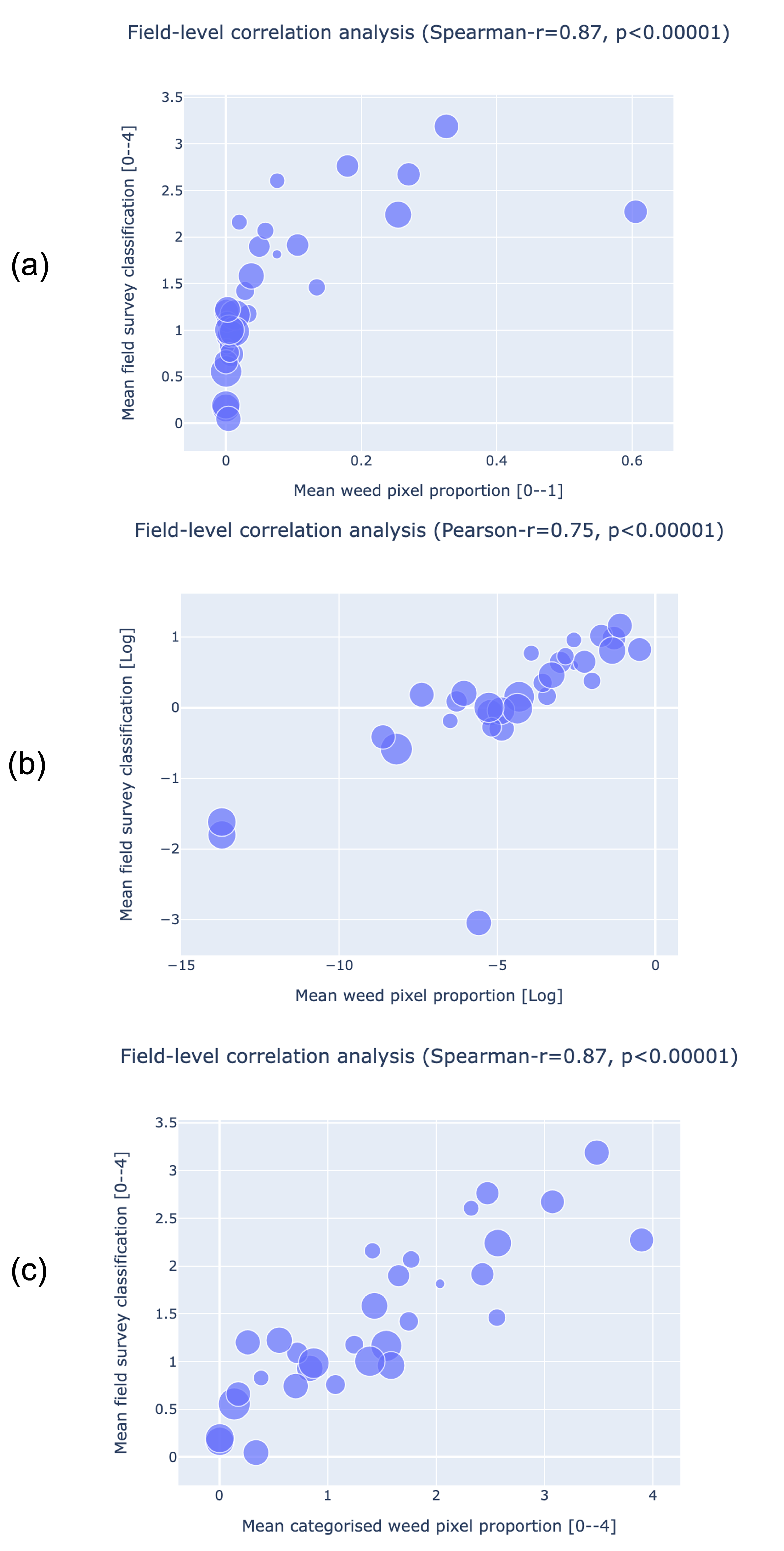
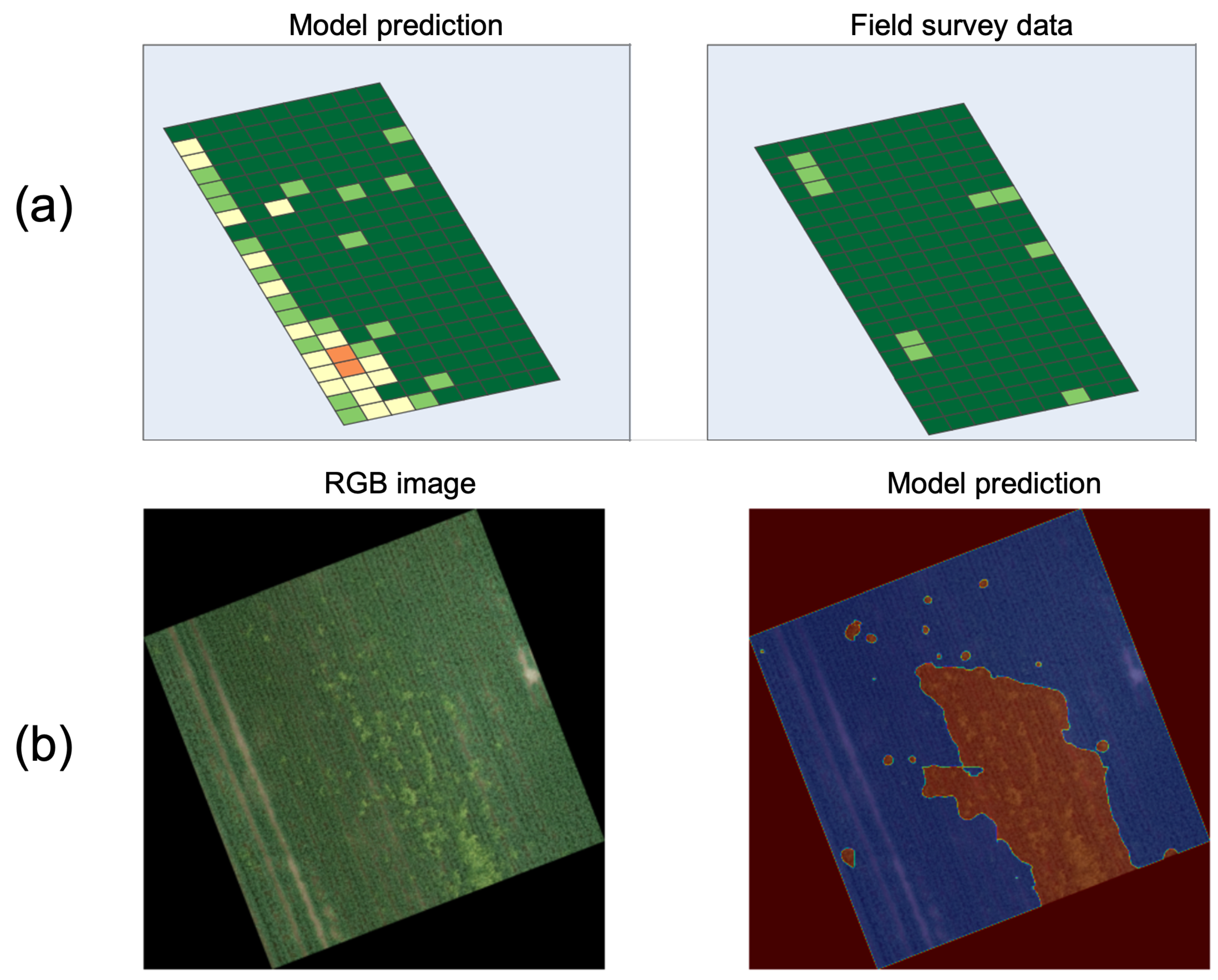
Figure 4 shows the results of the field-level correlation analysis (e.g., avarage value calculated for each field) between weed abundance as detected by the deep learning model (RGB-only model), versus the black-grass field survey data. All comparisons revealed a high and statistically significant correlation (i.e., ro > 0.75 and p < 0.00001). Comparing log-transformed abundances highlighted one particular outlier (Figure 4b), with a considerably greater model-derived mean quadrat weed pixel proportion than the mean black-grass density state recorded field. However, after further investigation (see Figure 5), this discrepancy was due to the fact that the field survey team targeted only one specific weed species (i.e., black-grass) while the model was also correctly identifying the presence of other similar weed species (Figure 5b)—in this case a brome (Bromus sp.).

3.3. Model Deployment Pathway

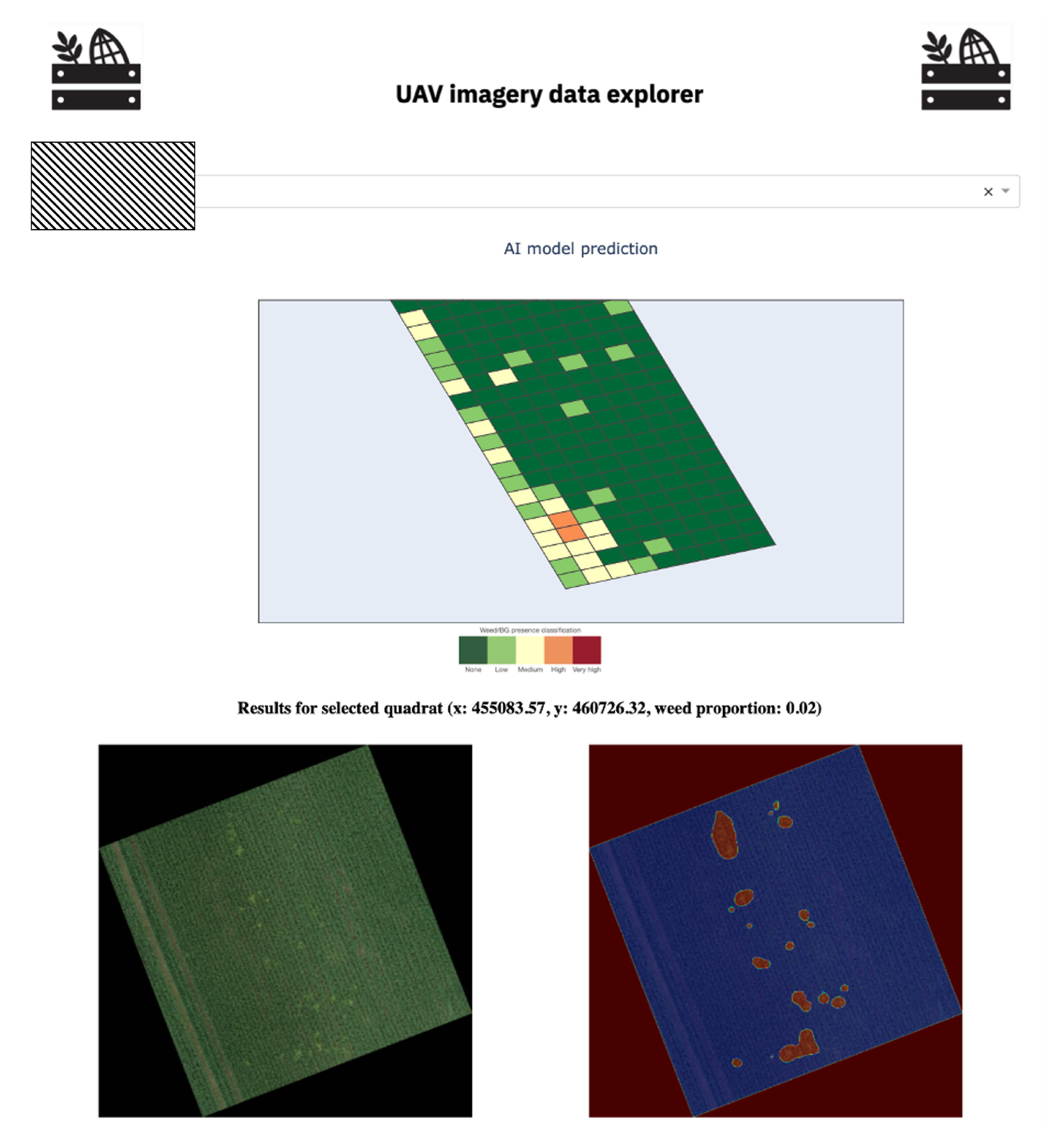
To make the model usable, we created a lightweight Docker container that only needs the path to newly collected data to predict on (e.g., field RGB image collected with UAV). For example, this took 22 min to process the RGB of a new field of size 2.5 hectares, on a Power8 system with a single GPU, 20 cores and 64 Gb of RAM. The docker container could be made fully operational via a simple API or just used locally (e.g., it works with and without Graphical Processing Units) by analysts and agronomists. Once categorised, the output is then accessible via a simple dashboard, e.g., Figure 6, providing an easily understandable overall view of the weed abundance in the field. This map is also clickable, giving the user the chance to explore the results to gain confidence in the model predictions. Furthermore, the data used to build this map, which contain geolocated weed abundance, could be easily exported and made available to on-farm machinery to support targeted herbicide applications.

4. Discussion

4.1. Summary

We created and validated a deep learning model to detect the spatial extent of weeds from UAV imagery in winter wheat in the UK. The performance of our model, based on a large out-of-bag dataset composed of 34 fields, showed high accuracy and good performance for a model detecting grass-weeds in a narrow-row grass crop. Model accuracy was higher than 0.90, and validation of model predictions against field ground truth data for the weed black-grass, collected by experts over 205 hectares, revealed good concordance between the imagery-derived weed maps and field surveillance, especially for field-level weed mapping (i.e., ro > 0.75 and p < 0.00001). Although results had a tendency to over-predict around found patches, (and with no improvement introduced by using multispectral data), model performance could likely be further improved through more precise data annotation. Finally, we have demonstrated how such a model can easily be deployed with a lightweight Docker container, and propose a dashboard prototype to give easy access to farmers.

4.2. Comparison to Previous Literature

Detection of grassweed species in narrow-row cereal cropping situations is notoriously difficult due to the weed and crop sharing similar morphological and spectral properties [22,27]. Black-grass provides some opportunity for detection for a short time (~1 month) during flowering, as the weed flowering heads emerge above the crop. Nevertheless, to the best of our knowledge, only two recent studies have attempted to identify black-grass in winter wheat at a large scale [12,13]. Both prior studies tackled this as a classification problem, trying to predict the abundance class directly, while these attempts showed some promise, both studies obtained low out-of-bag performance when validating their models. Here we demonstrate that an approach using image segmentation, rather than classification, with a high image resolution, can lead to useful predictions on unseen field ground truth data. Good model performance using image segmentation was also reported by Jinya et al. [17] who used a Random Forest approach on multispectral UAV imagery to detect black-grass pixels in a winter wheat crop. However, the model and dataset reported here provide some important advantages over such previous work. The model reported by Jinya et al. [17] refers to data from only a single field, and surveillance of such small areas or small experimental plots predominates in studies of remote weed mapping [28]. The current model based on assessment of 34 fields represents one of the largest studies of this kind, and highlights the importance of future model development to prioritise the generalisability of models to improve out-of-bag performance (i.e., between fields), something which is often overlooked by smaller-scale studies. Additionally, here we report good model performance against criteria derived from both post hoc annotation, and actual field observations, something lacking from the vast majority of current published studies [10].

4.3. Lessons Learned

Ecological research into population dynamics is currently constrained by the expense in time and resources required to accurately survey large areas, meaning that most studies are based on small detailed surveys of single or few populations [5,39]. Importantly, the results shown here demonstrate a strong correlation between the binned, model-derived weed abundance predictions, and the standard density-structured survey methodology used for ecological research of A. myosuroides [6]. This form of density-structured weed data is invaluable for study of weed spatio-temporal dynamics, as it allows data of sufficient detail and resolution for ecological modelling to be collected over a relatively large area [30]. However this technique remains time consuming, and is also limited by the need for teams of trained field assessors. Our results demonstrate the utility of deep learning models and UAV imagery to capture equivalent density-structured information over large areas, raising the potential for this approach to facilitate larger scale ecological research into these species in future. As a result, while field surveillance will always be invaluable to provide true ‘ground-truth’ data for validation, the use of UAV derived remote mapping of weed populations should be explored further as a tool to supplement ongoing efforts into weed monitoring for ecological research.
From an agronomic perspective, one key use for weed mapping tools such as this is to underpin more sustainable, precision or variable-rate herbicide application [19,20,21]. Such approaches have dual benefits in terms of both reducing herbicide volumes used (thereby reducing the ecotoxicological consequences of spraying), and reducing costs to the farmer [3,4]. Nevertheless, uptake of such practices has remained low due to hesitance from growers around the potential to miss weed patches [40]. In this study, although some of the model metrics (i.e., IoU, F1-score and precision) were generally low when performance was calculated, visual inspection and qualitative analysis of the weed maps revealed that this was often due to over-prediction around found patches, or identification of plants or patches too small to be annotated while labelling the data, while reducing the reported model performance, this finding is actually less detrimental for real world agronomic use. The relatively conservative weed predictions demonstrated here help to ensure that small patches of weed are not overlooked, which could aid grower confidence in the resultant weed maps and help facilitate more widespread uptake of precision or variable rate application techniques.

4.4. Limitations

Overall, the model presented here provides a clear improvement on previous attempts to map this weed species remotely [12,13]. Nevertheless, there remain opportunities for future studies to take these results further. First, due to the size and amount of data collected, it was not feasible to label small patches or individual weed plants visible from the RGB data. As mentioned above, this led to some of the performance metrics to be low, despite the model correctly identifying presence of the weed. Novel approaches to incentivise or facilitate large-scale data annotation have been developed in other disciplines to overcome the hurdle of time-consuming, accurate annotation of imagery [41]. Utilising such approaches to facilitate accurate annotation of large-scale weed imagery would help to improve both the training and validation of weed detection models in the future. Secondly, we focused on a single ResNet-UNET architecture for weed segmentation here, as this approach represents the most frequently used architecture in Earth Observation image segmentation tasks based on satellite and UAV imagery, as well as being widely used in weed detection from a range of different sensors [7,36]. Nevertheless, future studies comparing different detection algorithms might help to identify approaches which could further improve accuracy. Thirdly, as the fields surveyed here are predominantly infested with black-grass, images were only annotated with a single weed label class. In the few instances where other weed species are present (Bromus sp.), this has led to some discrepancy between the black-grass ground-truth data and the model outputs. In theory, future models could be trained to distinguish multiple independent weed species, e.g., de Camargo et al. [23], and further work is warranted on fields with communities of multiple weed species to explore this. Finally, we focused our analysis on winter wheat only. Focusing on a single crop is pragmatic from the perspective of ensuring a large dataset with minimal variability, and winter wheat is both one of the most frequently grown cash crops in the UK, and the crop most affected by black-grass [13,29,30]. Nevertheless, there remains the potential to explore detection of this species in other cropping situations such as barley (Hordeum vulgare) or oilseed rape (Brassica napus), or at other earlier developmental times.

4.5. Future Directions

For the future, we will take advantage of our deployable model and user interface to seek opportunities for real world use in the summer 2022 season. Furthermore, from a technical perspective, we plan to further develop our approach by testing custom deep learning architectures that might be able to take full advantage of the multispectral data we collected, and assess whether extra field-dependent features (e.g., soil type and temperature) might further improve predictions.

5. Conclusions

Deep learning is a potentially disruptive technology that to date, has not received widespread adoption for weed detection in the real-world due to limitations around data collection, quality and size. Here, we have demonstrated that a deep learning approach applied to weed detection in UK cereal cropping can provide accurate predictions (model accuracy > 0.9 on true out-of-bag data) using imagery-derived local and global weed maps, and statistically significant correlations (i.e., ro > 0.75 and p < 0.00001) against field ground-truth survey data. In doing so, this study demonstrates the utility of deep learning for accurate surveillance of problematic weed species in the field. As such, our study represents a concrete example of how these limitations can be overcome, and how deep learning model predictions, validated at scale, can be used for both ecological research and to enhance agronomic decision making.

Author Contributions

Conceptualization, P.F., D.C., K.R. and B.E.; methodology, P.F. and D.C.; data labelling/curation, P.F., D.C., K.R. and J.B.; data analysis, P.F. and D.C.; writing original draft preparation, P.F. and D.C.; writing review and editing, P.F., D.C., K.R., B.E., J.B., D.Z.C. and R.P.F. All authors have read and agreed to the published version of the manuscript.

Funding

This project was funded by Innovate UK via the “aiScope—AI data platform for smart crop protection” grant (Reference number: 105145).

Data Availability Statement

Restrictions apply to the availability of these data. Data was obtained as part of the aiScope project and are available from the authors with the permission of the whole consortium.

Acknowledgments

We thank Hummingbird Technologies (https://hummingbirdtech.com/, accessed on 17 July 2022) for their support and collaboration during the UAV data collection.

Conflicts of Interest

The authors declare no conflict of interest.

References

  1. Oerke, E.C. Crop losses to pests. J. Agric. Sci. 2006, 144, 31–43. [Google Scholar] [CrossRef]
  2. Varah, A.; Ahodo, K.; Coutts, S.R.; Hicks, H.L.; Comont, D.; Crook, L.; Hull, R.; Neve, P.; Childs, D.Z.; Freckleton, R.P. The costs of human-induced evolution in an agricultural system. Nat. Sustain. 2020, 3, 63–71. [Google Scholar] [CrossRef]
  3. Franco, C.; Pedersen, S.; Papaharalampos, H.; Ørum, J. The value of precision for image-based decision support in weed management. Precis. Agric. 2017, 18, 366–382. [Google Scholar] [CrossRef]
  4. Hamouz, P.; Hamouzová, K.; Holec, J.; Tyšer, L. Impact of site-specific weed management on herbicide savings and winter wheat yield. Plant Soil Environ. 2013, 59, 101–107. [Google Scholar] [CrossRef]
  5. Qi, A.; Perry, J.; Pidgeon, J.; Haylock, L.; Brooks, D. Cost-efficacy in measuring farmland biodiversity–lessons from the Farm Scale Evaluations of genetically modified herbicide-tolerant crops. Ann. Appl. Biol. 2008, 152, 93–101. [Google Scholar] [CrossRef]
  6. Queenborough, S.A.; Burnet, K.M.; Sutherland, W.J.; Watkinson, A.R.; Freckleton, R.P. From meso-to macroscale population dynamics: A new density-structured approach. Methods Ecol. Evol. 2011, 2, 289–302. [Google Scholar] [CrossRef]
  7. Hoeser, T.; Bachofer, F.; Kuenzer, C. Object detection and image segmentation with deep learning on Earth observation data: A review—Part II: Applications. Remote Sens. 2020, 12, 3053. [Google Scholar] [CrossRef]
  8. Huang, H.; Deng, J.; Lan, Y.; Yang, A.; Deng, X.; Wen, S.; Zhang, H.; Zhang, Y. Accurate weed mapping and prescription map generation based on fully convolutional networks using UAV imagery. Sensors 2018, 18, 3299. [Google Scholar] [CrossRef] [PubMed]
  9. Huang, Y.; Reddy, K.N.; Fletcher, R.S.; Pennington, D. UAV low-altitude remote sensing for precision weed management. Weed Technol. 2018, 32, 2–6. [Google Scholar] [CrossRef]
  10. Mohidem, N.A.; Che’Ya, N.N.; Juraimi, A.S.; Fazlil Ilahi, W.F.; Mohd Roslim, M.H.; Sulaiman, N.; Saberioon, M.; Mohd Noor, N. How Can Unmanned Aerial Vehicles Be Used for Detecting Weeds in Agricultural Fields? Agriculture 2021, 11, 1004. [Google Scholar] [CrossRef]
  11. Sa, I.; Popović, M.; Khanna, R.; Chen, Z.; Lottes, P.; Liebisch, F.; Nieto, J.; Stachniss, C.; Walter, A.; Siegwart, R. WeedMap: A large-scale semantic weed mapping framework using aerial multispectral imaging and deep neural network for precision farming. Remote Sens. 2018, 10, 1423. [Google Scholar] [CrossRef]
  12. Lambert, J.; Hicks, H.; Childs, D.; Freckleton, R. Evaluating the potential of Unmanned Aerial Systems for mapping weeds at field scales: A case study with Alopecurus myosuroides. Weed Res. 2018, 58, 35–45. [Google Scholar] [CrossRef] [PubMed]
  13. Lambert, J.P.; Childs, D.Z.; Freckleton, R.P. Testing the ability of unmanned aerial systems and machine learning to map weeds at subfield scales: A test with the weed Alopecurus myosuroides (Huds). Pest Manag. Sci. 2019, 75, 2283–2294. [Google Scholar] [CrossRef] [PubMed]
  14. Jurado-Expósito, M.; López-Granados, F.; Jiménez-Brenes, F.M.; Torres-Sánchez, J. Monitoring the Spatial Variability of Knapweed (Centaurea diluta Aiton) in Wheat Crops Using Geostatistics and UAV Imagery: Probability Maps for Risk Assessment in Site-Specific Control. Agronomy 2021, 11, 880. [Google Scholar] [CrossRef]
  15. Rozenberg, G.; Kent, R.; Blank, L. Consumer-grade UAV utilized for detecting and analyzing late-season weed spatial distribution patterns in commercial onion fields. Precis. Agric. 2021, 22, 1317–1332. [Google Scholar] [CrossRef]
  16. Zou, K.; Chen, X.; Zhang, F.; Zhou, H.; Zhang, C. A Field Weed Density Evaluation Method Based on UAV Imaging and Modified U-Net. Remote Sens. 2021, 13, 310. [Google Scholar] [CrossRef]
  17. Jinya, S.; Yi, D.; Coombes, M.; Liu, C.; Zhai, X.; McDonald-Maier, K.; Chen, W.H. Spectral analysis and mapping of blackgrass weed by leveraging machine learning and UAV multispectral imagery. Comput. Electron. Agric. 2022, 192, 106621. [Google Scholar]
  18. López-Granados, F.; Torres-Sánchez, J.; Serrano-Pérez, A.; de Castro, A.I.; Mesas-Carrascosa, F.J.; Pena, J.M. Early season weed mapping in sunflower using UAV technology: Variability of herbicide treatment maps against weed thresholds. Precis. Agric. 2016, 17, 183–199. [Google Scholar] [CrossRef]
  19. Castaldi, F.; Pelosi, F.; Pascucci, S.; Casa, R. Assessing the potential of images from unmanned aerial vehicles (UAV) to support herbicide patch spraying in maize. Precis. Agric. 2017, 18, 76–94. [Google Scholar] [CrossRef]
  20. Nikolić, N.; Rizzo, D.; Marraccini, E.; Gotor, A.A.; Mattivi, P.; Saulet, P.; Persichetti, A.; Masin, R. Site and time-specific early weed control is able to reduce herbicide use in maize-a case study. Ital. J. Agron. 2021, 16, 1780. [Google Scholar] [CrossRef]
  21. Hunter, J.E., III; Gannon, T.W.; Richardson, R.J.; Yelverton, F.H.; Leon, R.G. Integration of remote-weed mapping and an autonomous spraying unmanned aerial vehicle for site-specific weed management. Pest Manag. Sci. 2020, 76, 1386–1392. [Google Scholar] [CrossRef] [PubMed] [Green Version]
  22. Fernández-Quintanilla, C.; Peña, J.; Andújar, D.; Dorado, J.; Ribeiro, A.; López-Granados, F. Is the current state of the art of weed monitoring suitable for site-specific weed management in arable crops? Weed Res. 2018, 58, 259–272. [Google Scholar] [CrossRef]
  23. de Camargo, T.; Schirrmann, M.; Landwehr, N.; Dammer, K.H.; Pflanz, M. Optimized Deep Learning Model as a Basis for Fast UAV Mapping of Weed Species in Winter Wheat Crops. Remote Sens. 2021, 13, 1704. [Google Scholar] [CrossRef]
  24. Liu, J.; Xiang, J.; Jin, Y.; Liu, R.; Yan, J.; Wang, L. Boost Precision Agriculture with Unmanned Aerial Vehicle Remote Sensing and Edge Intelligence: A Survey. Remote Sens. 2021, 13, 4387. [Google Scholar] [CrossRef]
  25. Peña, J.M.; Torres-Sánchez, J.; Serrano-Pérez, A.; De Castro, A.I.; López-Granados, F. Quantifying Efficacy and Limits of Unmanned Aerial Vehicle (UAV) Technology for Weed Seedling Detection as Affected by Sensor Resolution. Sensors 2015, 15, 5609–5626. [Google Scholar] [CrossRef]
  26. Che’Ya, N.N.; Dunwoody, E.; Gupta, M. Assessment of Weed Classification Using Hyperspectral Reflectance and Optimal Multispectral UAV Imagery. Agronomy 2021, 11, 1435. [Google Scholar] [CrossRef]
  27. Martin, M.P.; Barreto, L.; Riaño, D.; Fernandez-Quintanilla, C.; Vaughan, P. Assessing the potential of hyperspectral remote sensing for the discrimination of grassweeds in winter cereal crops. Int. J. Remote Sens. 2011, 32, 49–67. [Google Scholar] [CrossRef]
  28. Kaivosoja, J.; Hautsalo, J.; Heikkinen, J.; Hiltunen, L.; Ruuttunen, P.; Näsi, R.; Niemeläinen, O.; Lemsalu, M.; Honkavaara, E.; Salonen, J. Reference Measurements in Developing UAV Systems for Detecting Pests, Weeds, and Diseases. Remote Sens. 2021, 13, 1238. [Google Scholar] [CrossRef]
  29. Moss, S.R.; Perryman, S.A.; Tatnell, L.V. Managing herbicide-resistant blackgrass (Alopecurus myosuroides): Theory and practice. Weed Technol. 2007, 21, 300–309. [Google Scholar] [CrossRef]
  30. Hicks, H.L.; Comont, D.; Coutts, S.R.; Crook, L.; Hull, R.; Norris, K.; Neve, P.; Childs, D.Z.; Freckleton, R.P. The factors driving evolved herbicide resistance at a national scale. Nat. Ecol. Evol. 2018, 2, 529–536. [Google Scholar] [CrossRef]
  31. OpenVINO. Computer Vision Annotation Tool (CVAT). Available online: https://github.com/openvinotoolkit/cvat (accessed on 17 July 2022).
  32. Howard, J.; Gugger, S. Fastai: A layered API for deep learning. Information 2020, 11, 108. [Google Scholar] [CrossRef] [Green Version]
  33. Paszke, A.; Gross, S.; Massa, F.; Lerer, A.; Bradbury, J.; Chanan, G.; Killeen, T.; Lin, Z.; Gimelshein, N.; Antiga, L. Pytorch: An imperative style, high-performance deep learning library. arXiv 2019, arXiv:1912.01703. [Google Scholar]
  34. Ronneberger, O.; Fischer, P.; Brox, T. U-Net: Convolutional Networks for Biomedical Image Segmentation; Springer: Berlin/Heidelberg, Germany, 2015; pp. 234–241. [Google Scholar]
  35. He, K.; Zhang, X.; Ren, S.; Sun, J. Deep residual learning for image recognition. In Proceedings of the 2016 IEEE Conference on Computer Vision and Pattern Recognition (CVPR), Las Vegas, NV, USA, 27–30 June 2016; pp. 770–778. [Google Scholar]
  36. Zhangnan, W.; Chen, Y.; Zhao, B.; Kang, X.; Ding, Y. Review of weed detection methods based on computer vision. Sensors 2021, 11, 3647. [Google Scholar]
  37. Smith, L.N.; Topin, N. Super-convergence: Very fast training of neural networks using large learning rates. Int. Soc. Opt. Photonics 2019, 11006, 1100612. [Google Scholar]
  38. Wright, L. New Deep Learning Optimizer, Ranger: Synergistic Combination of RAdam + Look Ahead for the Best of Both. 2019. Available online: https://lessw.medium.com/new-deep-learning-optimizer-ranger-synergistic-combination-of-radam-lookahead-for-the-best-of-2dc83f79a48d (accessed on 17 July 2022).
  39. Gurevitch, J.; Fox, G.A.; Fowler, N.L.; Graham, C.H. Landscape Demography: Population Change and its Drivers Across Spatial Scales. Q. Rev. Biol. 2016, 91, 459–485. [Google Scholar] [CrossRef] [PubMed]
  40. Somerville, G.J.; Sønderskov, M.; Mathiassen, S.K.; Metcalfe, H. Spatial modelling of within-field weed populations; a review. Agronomy 2020, 10, 1044. [Google Scholar] [CrossRef]
  41. Balducci, F.; Buono, P. Building a Qualified Annotation Dataset for Skin Lesion Analysis Trough Gamification. In Proceedings of the 2018 International Conference on Advanced Visual Interfaces, AVI ’18, Riva del Sole, Italy, 29 May–1 June 2018; Association for Computing Machinery: New York, NY, USA, 2018. [Google Scholar] [CrossRef] [Green Version]
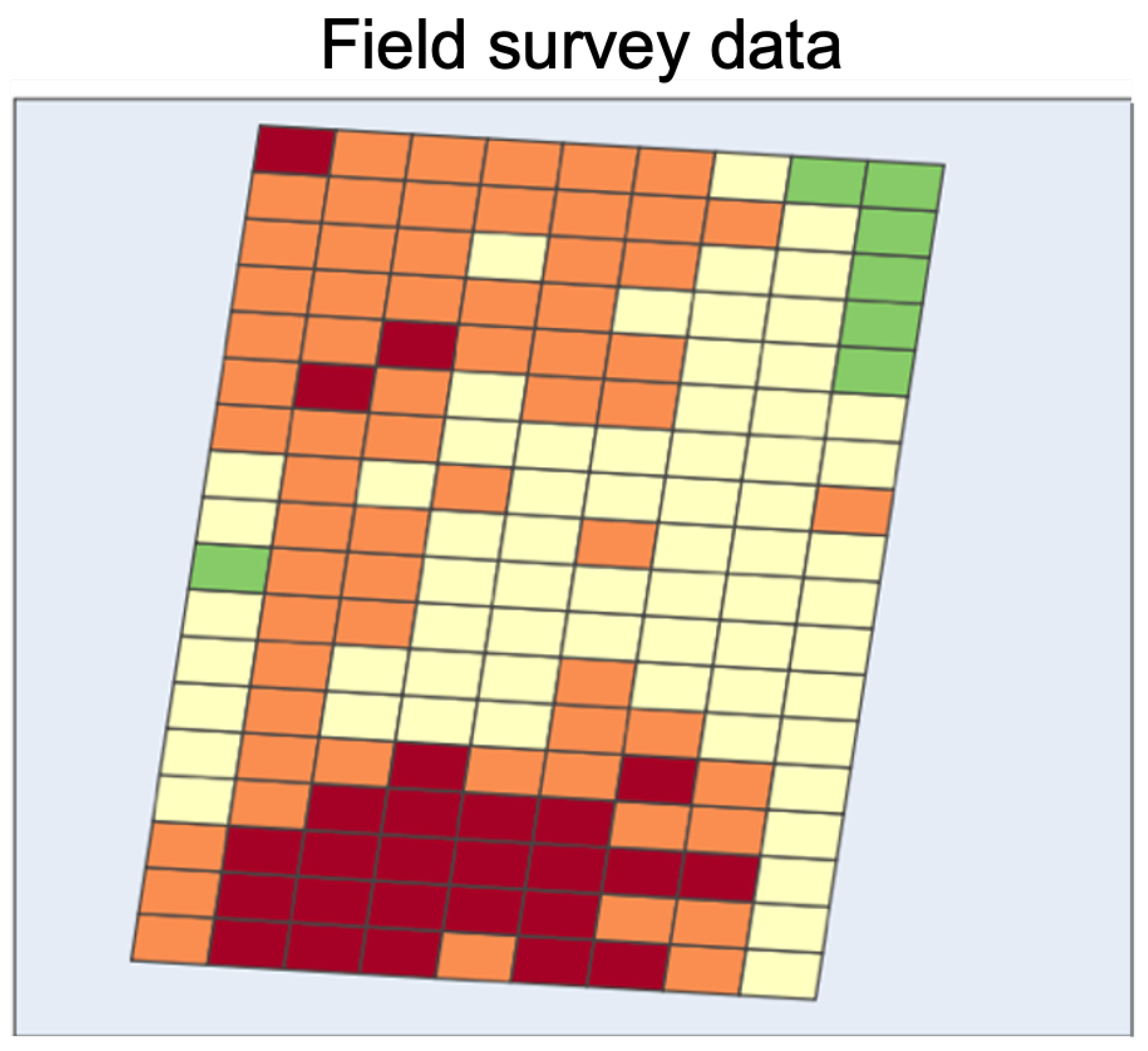
Figure 1. Example of field survey data collected for one field (dark green: absent; Light green: low; yellow: medium; orange: high; red: very high).
Remotesensing 14 04197 g001
Figure 2. Examples of model predictions for five fields. 1st column: original RGB image (weed represented by yellow and light green plants); 2nd column: target labels overlaid over RGB images; 3rd column: model prediction overlaid over RGB images.
Remotesensing 14 04197 g002
Figure 3. Quadrats weed pixel proportion distribution, as identified by the deep learning model (e.g., using 0.5 as a probability threshold to identify weed pixels) and compared to black-grass field survey data (0: none (N = 920); 1: low (N = 2848); 2: medium (N = 606); 3: high (N = 470); 4: very high (N = 288)).
Remotesensing 14 04197 g003
Figure 4. Field level correlation analysis (marker size indicates field size): (a) correlation analysis between field-level mean deep-learning weed pixel proportion in each quadrat and the field-level mean field survey data classification; (b) correlation analysis between the log-transformed field-level mean deep learning-derived weed pixel proportion in each quadrat and the log-trasformed field-level mean field survey data classification; (c) correlation analysis between field-level mean deep learning-derived weed pixel proportion derived classification in each quadrat and the field-level mean field survey data classification.
Remotesensing 14 04197 g004
Figure 5. (a) Comparison between classification derived from the deep learning model and field survey data for the outlier field in the correlation analysis (dark green: absent; Light green: low; yellow: medium; orange: high; red: very high); (b) closer look to one of the quadrats classified as high abundance of weed in (a) (e.g., orange) in terms of raw RGB image and related model prediction.
Remotesensing 14 04197 g005
Figure 6. Client dashboard example. Top: clickable weed abundance map based on model predictions and field survey categories (dark green: absent; Light green: low; yellow: medium; orange: high; red: very high). Bottom: weed model prediction on a specific tile.
Remotesensing 14 04197 g006
Table 1. Results shown as mean and standard deviation over all cross validation iterations for the RGB-only model.
DatasetMetricValue (Std)
Test setAccuracy0.92 (0.01)
IoU0.40 (0.03)
F1-score0.57 (0.03)
Recall0.89 (0.02)
Precision0.41 (0.03)
Out-of-bag setAccuracy0.91 (0.05)
IoU0.31 (0.09)
F1-score0.46 (0.11)
Recall0.72 (0.23)
Precision0.35 (0.06)
Table 2. Results shown as mean and standard deviation over all cross validation iterations for the RGB + multispectral model.
DatasetMetricValue (Std)
Test setAccuracy0.92 (0.01)
IoU0.40 (0.02)
F1-score0.57 (0.02)
Recall0.88 (0.04)
Precision0.42 (0.02)
Out-of-bag setAccuracy0.91 (0.03)
IoU0.30 (0.13)
F1-score0.45 (0.15)
Recall0.72 (0.27)
Precision0.35 (0.11)
Publisher’s Note: MDPI stays neutral with regard to jurisdictional claims in published maps and institutional affiliations.