
A Systematic Classification Method for Grassland Community Division Using China’s ZY1-02D Hyperspectral Observations


 ,
,
Abstract
:
1. Introduction
2. Materials
2.1. Experimental Data
2.1.1. ZY1-02D Hyperspectral Data and Preprocessing
2.1.2. Hyperspectral Data Preprocessing
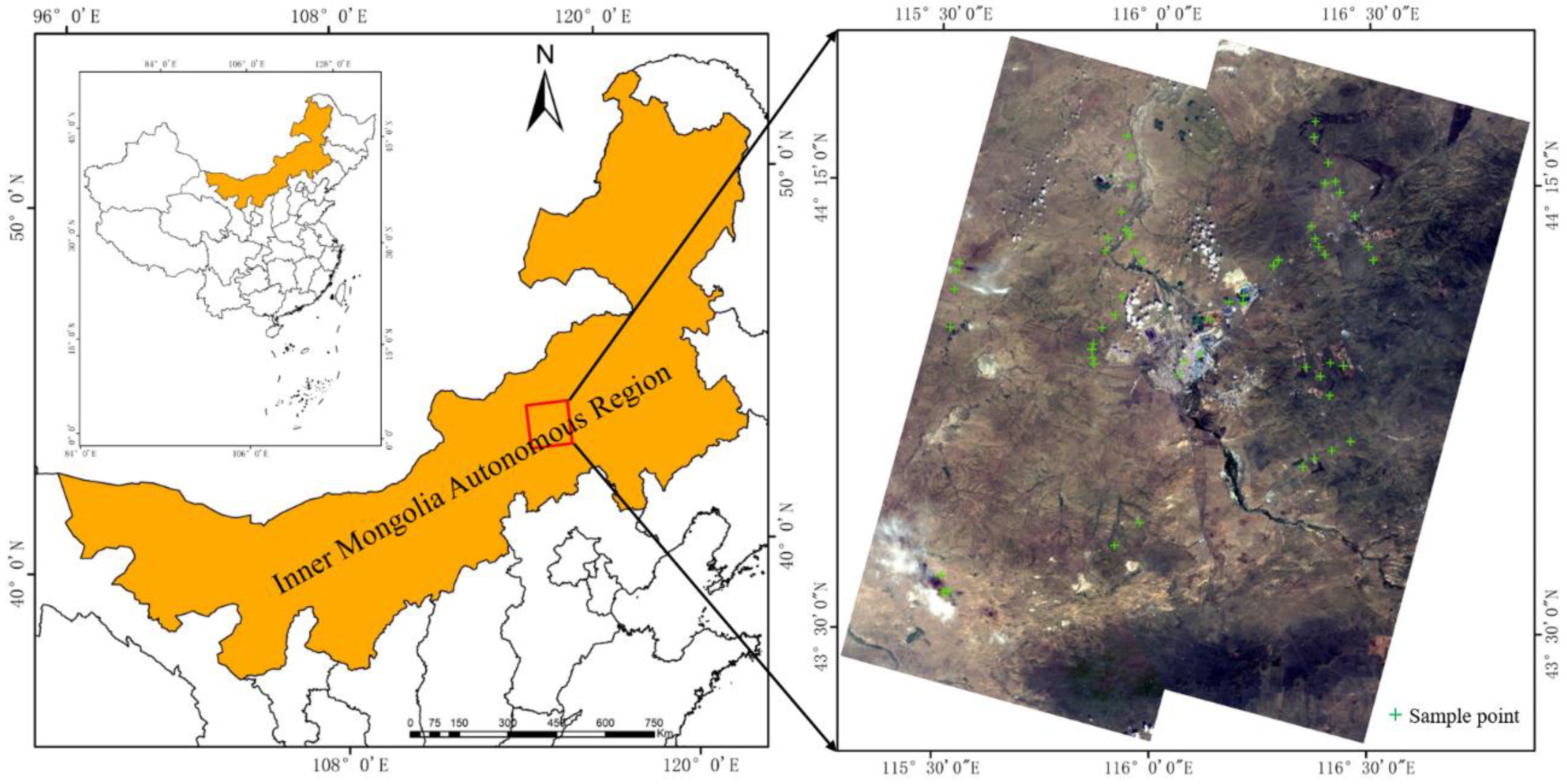
2.2. Study Area
2.3. Auxiliary Data
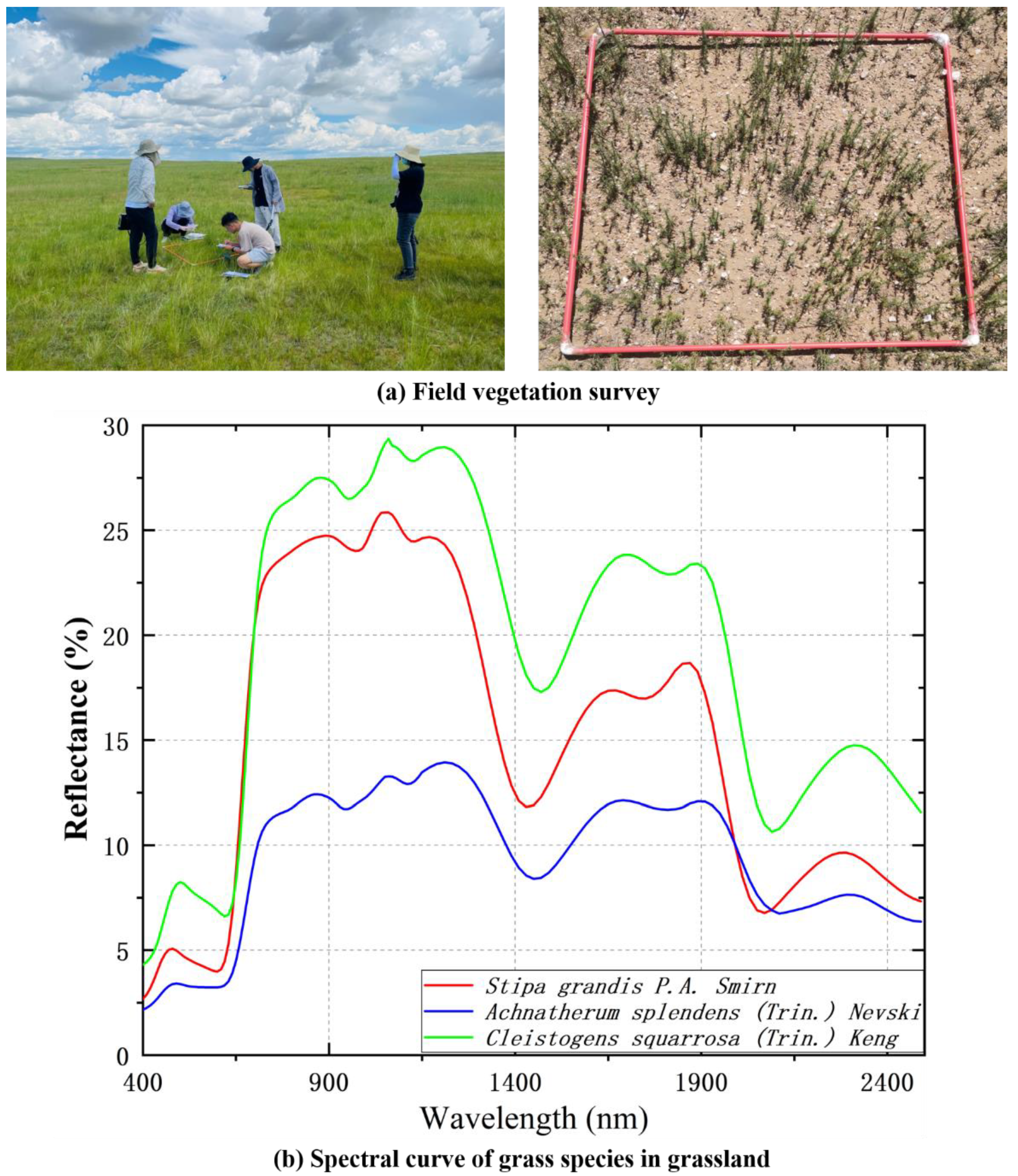
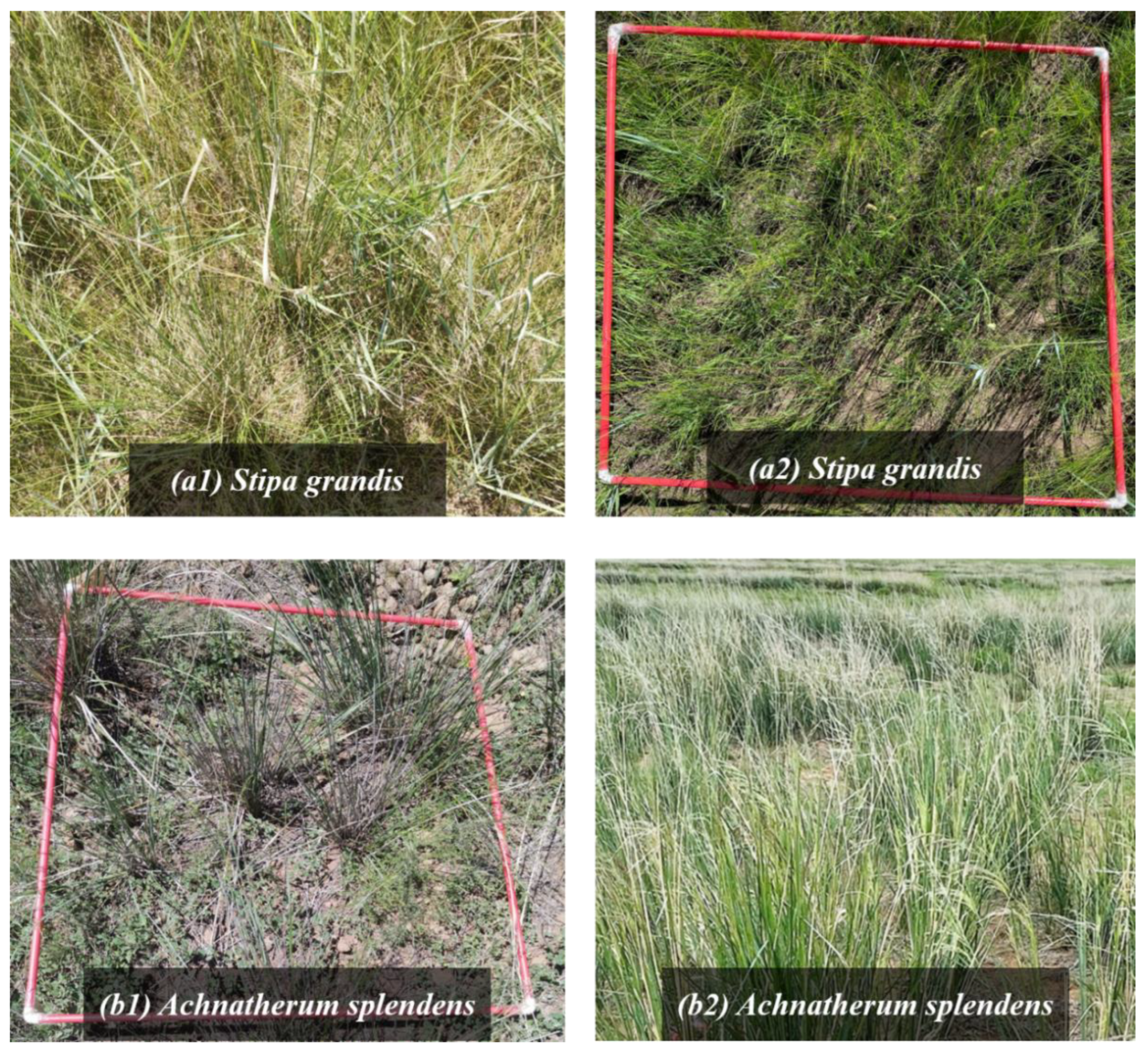
2.3.1. Field Survey Data
2.3.2. Updated Vegetation Map of China (1:1,000,000)
2.3.3. Functional Zoning Data of the Nature Reserves
3. Methods
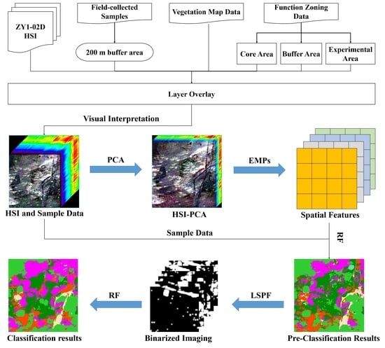
3.1. Overview
3.2. Sample Label Data Acquisition
3.3. Extracting Spatial Features of the Xilinhot Grassland Using EMPs
3.4. Classification Postprocessing Using LSPF
4. Experimental Results and Discussion
4.1. Experimental Setup
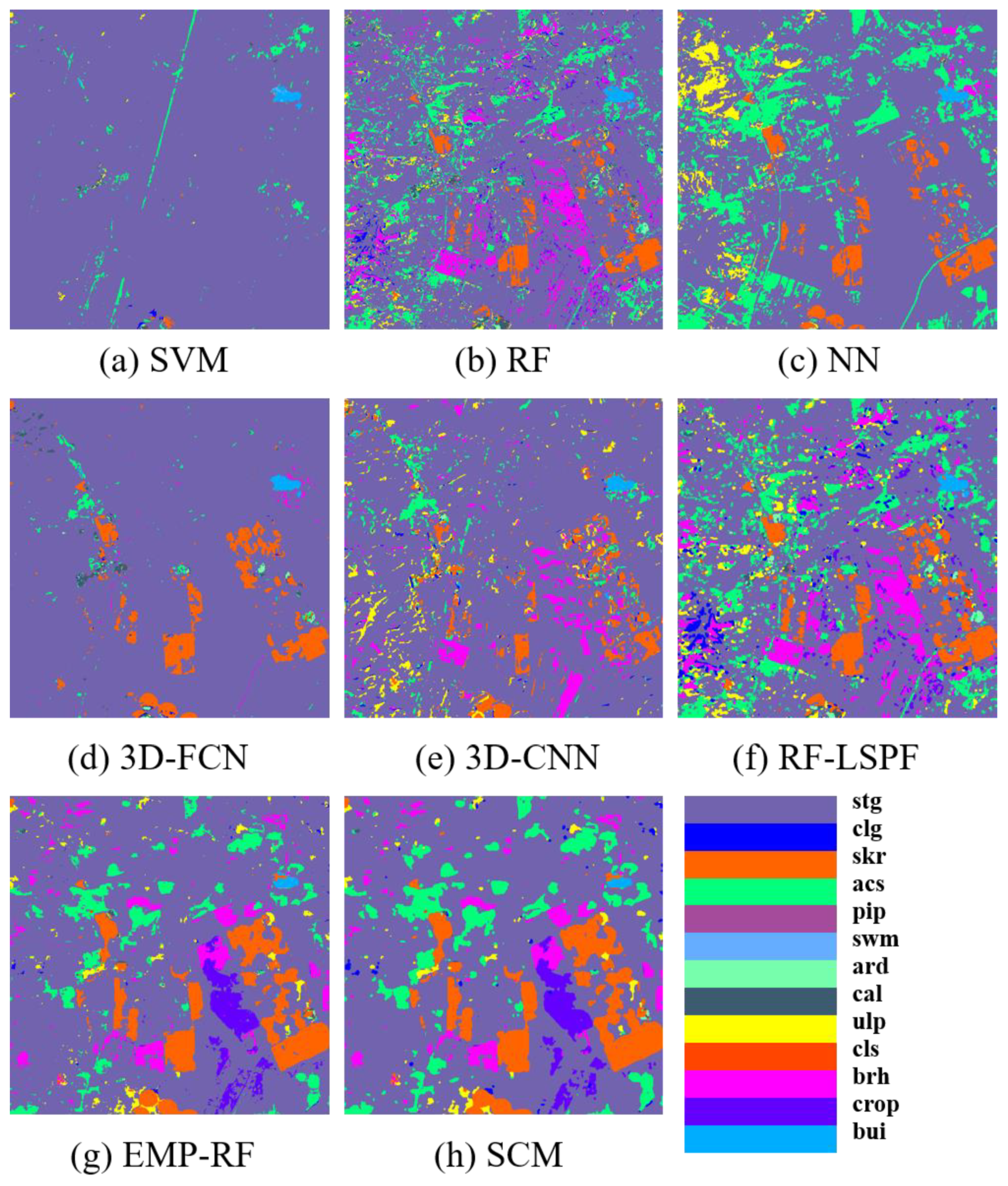
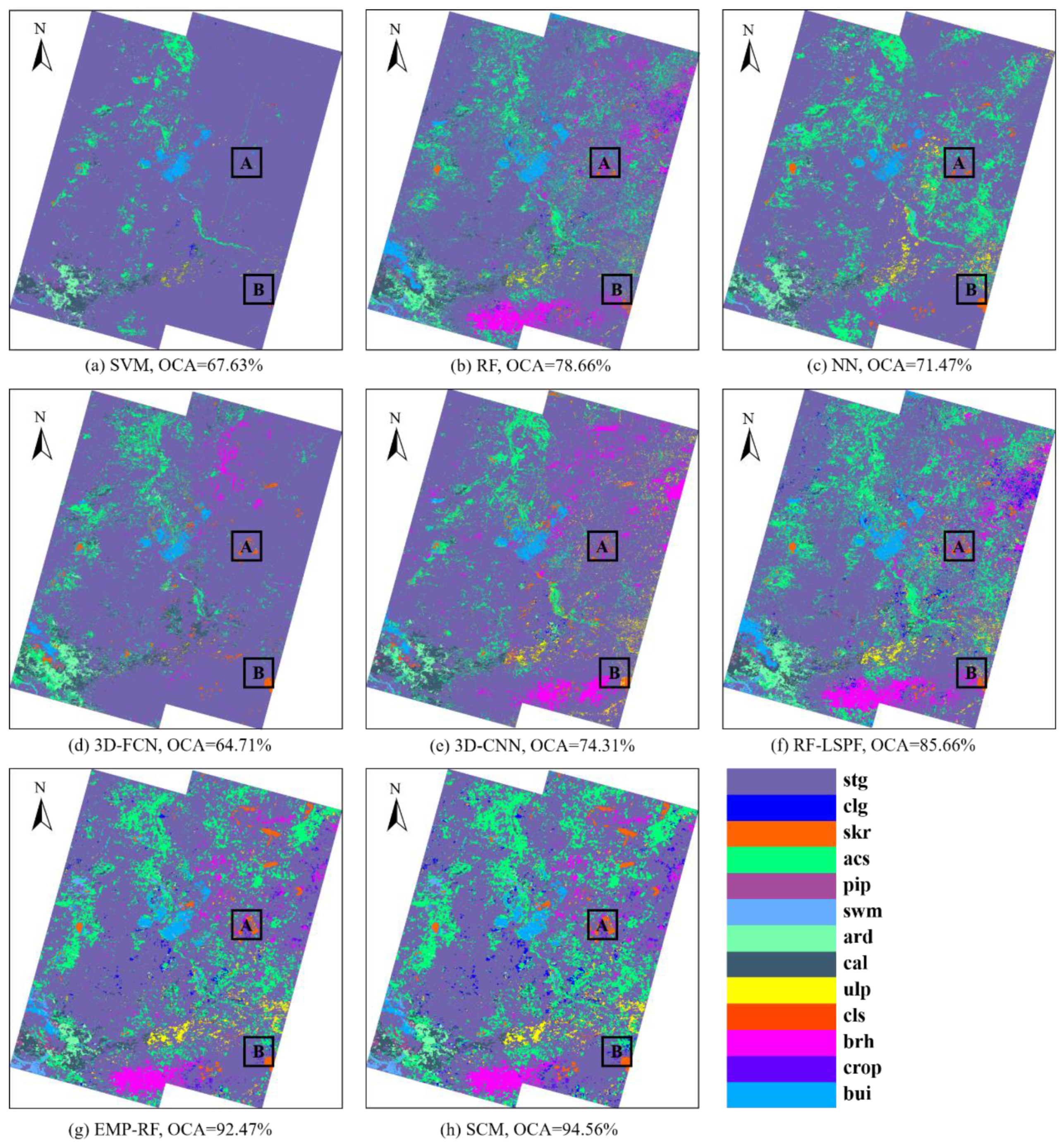
4.2. Classification Accuracy and Mapping Results
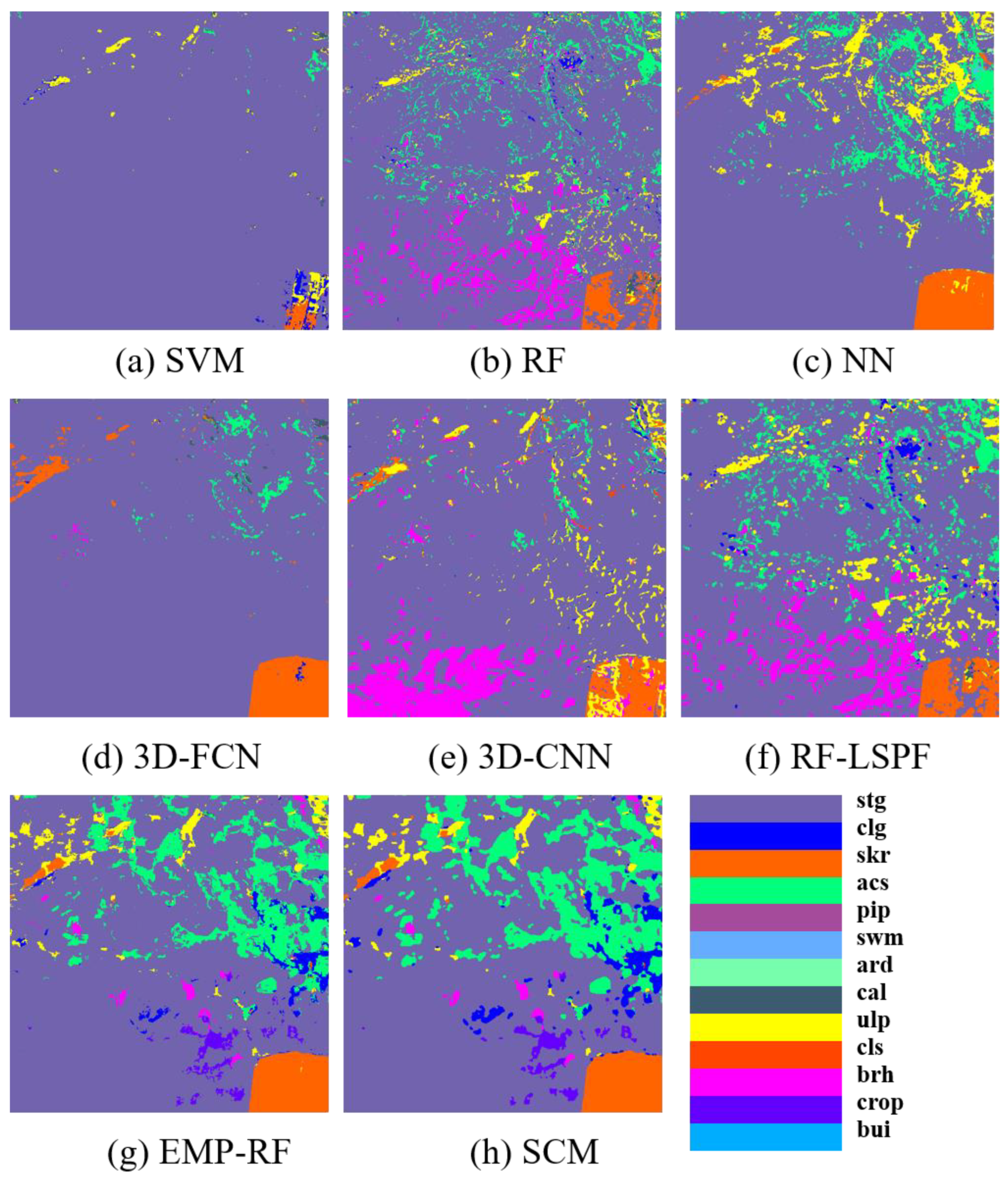
4.3. Typical Area Analysis
4.4. Disadvantages of Hyperspectral Images
5. Conclusions
Author Contributions
Funding
Data Availability Statement
Conflicts of Interest
References
- Zhou, W.; Gang, C.; Zhou, L.; Chen, Y.; Li, J.; Ju, W.; Odeh, I. Dynamic of grassland vegetation degradation and its quantitative assessment in the northwest China. Acta Oecologica 2014, 55, 86–96. [Google Scholar] [CrossRef]
- Liu, Y.; Wang, Q.; Zhang, Z.; Tong, L.; Wang, Z.; Li, J. Grassland dynamics in responses to climate variation and human activities in China from 2000 to 2013. Sci. Total Environ. 2019, 690, 27–39. [Google Scholar] [CrossRef] [PubMed]
- Chen, Y.; Mu, S.; Sun, Z.; Gang, C.; Li, J.; Padarian, J.; Groisman, P.; Chen, J.; Li, S. Grassland carbon sequestration ability in China: A new perspective from terrestrial aridity zones. Rangel. Ecol. Manag. 2016, 69, 84–94. [Google Scholar] [CrossRef]
- Emberson, L. Effects of ozone on agriculture, forests and grasslands. Philos. Trans. R. Soc. A 2020, 378, 20190327. [Google Scholar] [CrossRef]
- Zhou, W.; Yang, H.; Huang, L.; Chen, C.; Lin, X.; Hu, Z.; Li, J. Grassland degradation remote sensing monitoring and driving factors quantitative assessment in China from 1982 to 2010. Ecol. Indic. 2017, 83, 303–313. [Google Scholar] [CrossRef]
- He, C.; Tian, J.; Gao, B.; Zhao, Y. Differentiating climate-and human-induced drivers of grassland degradation in the Liao River Basin, China. Environ. Monit. Assess. 2015, 187, 4199. [Google Scholar] [CrossRef]
- Zhang, R.; Liang, T.; Guo, J.; Xie, H.; Feng, Q.; Aimaiti, Y. Grassland dynamics in response to climate change and human activities in Xinjiang from 2000 to 2014. Sci. Rep. 2018, 8, 2888. [Google Scholar] [CrossRef]
- Han, Z.; Song, W.; Deng, X.; Xu, X. Grassland ecosystem responses to climate change and human activities within the Three-River Headwaters region of China. Sci. Rep. 2018, 8, 9079. [Google Scholar] [CrossRef] [Green Version]
- Yu, C.; Zhang, Y.; Claus, H.; Zeng, R.; Zhang, X.; Wang, J. Ecological and environmental issues faced by a developing Tibet. ACS Publ. 2012, 46, 1979–1980. [Google Scholar] [CrossRef]
- Wu, J.; Mao, R.; Li, M.; Xia, J.; Song, J.; Cheng, D.; Sun, H. Assessment of aquatic ecological health based on determination of biological community variability of fish and macroinvertebrates in the Weihe River Basin, China. J. Environ. Manag. 2020, 267, 110651. [Google Scholar] [CrossRef]
- Jackson, R.B.; Canadell, J.; Ehleringer, J.R.; Mooney, H.; Sala, O.; Schulze, E.-D. A global analysis of root distributions for terrestrial biomes. Oecologia 1996, 108, 389–411. [Google Scholar] [CrossRef]
- Woodward, F.I.; Lomas, M.R.; Kelly, C.K. Global climate and the distribution of plant biomes. Philos. Trans. R. Soc. Lond. Ser. B Biol. Sci. 2004, 359, 1465–1476. [Google Scholar] [CrossRef] [Green Version]
- Mansour, K.; Mutanga, O.; Everson, T.; Adam, E. Discriminating indicator grass species for rangeland degradation assessment using hyperspectral data resampled to AISA Eagle resolution. ISPRS J. Photogramm. Remote Sens. 2012, 70, 56–65. [Google Scholar] [CrossRef]
- Li, B. Rangeland degradation in northern China and strategies for its prevention. Sci. Agric. Sin. 1997, 30, 1–8. [Google Scholar]
- Quangong, C. Current status and development of grassland monitoring in China. Pratacult. Sci. 2008, 25, 29–38. [Google Scholar]
- Cardellach, E.; Padullés, R.; Tomás, S.; Turk, F.; Ao, C.; de la Torre-Juárez, M. Probability of intense precipitation from polarimetric GNSS radio occultation observations. Q. J. R. Meteorol. Soc. 2018, 144, 206–220. [Google Scholar] [CrossRef] [Green Version]
- Song, D.; Zhen, Z.; Wang, B.; Li, X.; Gao, L.; Wang, N.; Xie, T.; Zhang, T. A novel marine oil spillage identification scheme based on convolution neural network feature extraction from fully polarimetric SAR imagery. IEEE Access 2020, 8, 59801–59820. [Google Scholar] [CrossRef]
- Toté, C.; Patricio, D.; Boogaard, H.; Van der Wijngaart, R.; Tarnavsky, E.; Funk, C. Evaluation of satellite rainfall estimates for drought and flood monitoring in Mozambique. Remote Sens. 2015, 7, 1758–1776. [Google Scholar] [CrossRef] [Green Version]
- Tian, H.; Wu, M.; Wang, L.; Niu, Z. Mapping early, middle and late rice extent using sentinel-1A and Landsat-8 data in the poyang lake plain, China. Sensors 2018, 18, 185. [Google Scholar] [CrossRef] [Green Version]
- Balogun, A.-L.; Yekeen, S.T.; Pradhan, B.; Althuwaynee, O.F. Spatio-temporal analysis of oil spill impact and recovery pattern of coastal vegetation and wetland using multispectral satellite landsat 8-OLI imagery and machine learning models. Remote Sens. 2020, 12, 1225. [Google Scholar] [CrossRef] [Green Version]
- Wang, X.; Gao, X.; Zhang, Y.; Fei, X.; Chen, Z.; Wang, J.; Zhang, Y.; Lu, X.; Zhao, H. Land-cover classification of coastal wetlands using the RF algorithm for Worldview-2 and Landsat 8 images. Remote Sens. 2019, 11, 1927. [Google Scholar] [CrossRef] [Green Version]
- Su, H.; Yao, W.; Wu, Z.; Zheng, P.; Du, Q. Kernel low-rank representation with elastic net for China coastal wetland land cover classification using GF-5 hyperspectral imagery. ISPRS J. Photogramm. Remote Sens. 2021, 171, 238–252. [Google Scholar] [CrossRef]
- San Martín, L.; Morandeira, N.S.; Grimson, R.; Rajngewerc, M.; González, E.B.; Kandus, P. The contribution of ALOS/PALSAR-1 multi-temporal data to map permanently and temporarily flooded coastal wetlands. Int. J. Remote Sens. 2020, 41, 1582–1602. [Google Scholar] [CrossRef]
- Shen, X.; Wang, D.; Mao, K.; Anagnostou, E.; Hong, Y. Inundation extent mapping by synthetic aperture radar: A review. Remote Sens. 2019, 11, 879. [Google Scholar] [CrossRef] [Green Version]
- Ishida, T.; Kurihara, J.; Viray, F.A.; Namuco, S.B.; Paringit, E.C.; Perez, G.J.; Takahashi, Y.; Marciano, J.J., Jr. A novel approach for vegetation classification using UAV-based hyperspectral imaging. Comput. Electron. Agric. 2018, 144, 80–85. [Google Scholar] [CrossRef]
- Audebert, N.; Le Saux, B.; Lefèvre, S. Deep learning for classification of hyperspectral data: A comparative review. IEEE Geosci. Remote Sens. Mag. 2019, 7, 159–173. [Google Scholar] [CrossRef] [Green Version]
- Hestir, E.L.; Brando, V.E.; Bresciani, M.; Giardino, C.; Matta, E.; Villa, P.; Dekker, A.G. Measuring freshwater aquatic ecosystems: The need for a hyperspectral global mapping satellite mission. Remote Sens. Environ. 2015, 167, 181–195. [Google Scholar] [CrossRef] [Green Version]
- Sun, W.; Liu, K.; Ren, G.; Liu, W.; Yang, G.; Meng, X.; Peng, J. A simple and effective spectral-spatial method for mapping large-scale coastal wetlands using China ZY1-02D satellite hyperspectral images. Int. J. Appl. Earth Obs. Geoinf. 2021, 104, 102572. [Google Scholar] [CrossRef]
- Carrizosa, E.; Morales, D.R. Supervised classification and mathematical optimization. Comput. Oper. Res. 2013, 40, 150–165. [Google Scholar] [CrossRef] [Green Version]
- Jiao, L.; Sun, W.; Yang, G.; Ren, G.; Liu, Y. A hierarchical classification framework of satellite multispectral/hyperspectral images for mapping coastal wetlands. Remote Sens. 2019, 11, 2238. [Google Scholar] [CrossRef] [Green Version]
- Le Bris, A.; Rosa, P.; Lerouxel, A.; Cognie, B.; Gernez, P.; Launeau, P.; Robin, M.; Barillé, L. Hyperspectral remote sensing of wild oyster reefs. Estuar. Coast. Shelf Sci. 2016, 172, 1–12. [Google Scholar] [CrossRef]
- Camps-Valls, G.; Gomez-Chova, L.; Munoz-Mari, J.; Vila-Frances, J.; Calpe-Maravilla, J. Composite kernels for hyperspectral image classification. IEEE Geosci. Remote Sens. Lett. 2006, 3, 93–97. [Google Scholar] [CrossRef]
- Li, W.; Du, Q. Joint Within-Class Collaborative Representation for Hyperspectral Image Classification. IEEE J. Sel. Top. Appl. Earth Obs. Remote Sens. 2014, 7, 2200–2208. [Google Scholar] [CrossRef]
- Gao, Q.; Lim, S.; Jia, X. Spectral–spatial hyperspectral image classification using a multiscale conservative smoothing scheme and adaptive sparse representation. IEEE Trans. Geosci. Remote Sens. 2019, 57, 7718–7730. [Google Scholar] [CrossRef]
- Cao, X.; Xu, Z.; Meng, D. Spectral-Spatial Hyperspectral Image Classification via Robust Low-Rank Feature Extraction and Markov Random Field. Remote Sens. 2019, 11, 1565. [Google Scholar] [CrossRef] [Green Version]
- Kang, X.; Li, S.; Benediktsson, J.A. Spectral–spatial hyperspectral image classification with edge-preserving filtering. IEEE Trans. Geosci. Remote Sens. 2013, 52, 2666–2677. [Google Scholar] [CrossRef]
- Song, W.; Li, S.; Fang, L.; Lu, T. Hyperspectral image classification with deep feature fusion network. IEEE Trans. Geosci. Remote Sens. 2018, 56, 3173–3184. [Google Scholar] [CrossRef]
- Xu, Y.; Du, B.; Zhang, L. Beyond the patchwise classification: Spectral-spatial fully convolutional networks for hyperspectral image classification. IEEE Trans. Big Data 2019, 6, 492–506. [Google Scholar] [CrossRef]
- Roy, S.K.; Manna, S.; Song, T.; Bruzzone, L. Attention-based adaptive spectral–spatial kernel ResNet for hyperspectral image classification. IEEE Trans. Geosci. Remote Sens. 2020, 59, 7831–7843. [Google Scholar] [CrossRef]
- Paoletti, M.; Haut, J.; Plaza, J.; Plaza, A. A new deep convolutional neural network for fast hyperspectral image classification. ISPRS J. Photogramm. Remote Sens. 2018, 145, 120–147. [Google Scholar] [CrossRef]
- Asghari Beirami, B.; Mokhtarzade, M. Spatial-Spectral Classification of Hyperspectral Images Based on Extended Morphological Profiles and Guided Filter. Comput. Knowl. Eng. 2020, 2, 2–8. [Google Scholar]
- Yu, J.; Liang, D.; Han, B.; Gao, H. Study on ground object classification based on the hyperspectral fusion images of ZY-1 (02D) satellite. J. Appl. Remote Sens. 2021, 15, 042603. [Google Scholar] [CrossRef]
- Lu, H.; Qiao, D.; Li, Y.; Wu, S.; Deng, L. Fusion of China ZY-1 02D Hyperspectral Data and Multispectral Data: Which Methods Should Be Used? Remote Sens. 2021, 13, 2354. [Google Scholar] [CrossRef]
- Xu, Z.; Chen, S.; Zhu, B.; Chen, L.; Ye, Y.; Lu, P. Evaluating the Capability of Satellite Hyperspectral Imager, the ZY1–02D, for Topsoil Nitrogen Content Estimation and Mapping of Farmlands in Black Soil Area, China. Remote Sens. 2022, 14, 1008. [Google Scholar] [CrossRef]
- Lyu, X.; Li, X.; Gong, J.; Wang, H.; Dang, D.; Dou, H.; Li, S.; Liu, S. Comprehensive grassland degradation monitoring by remote sensing in Xilinhot, Inner Mongolia, China. Sustainability 2020, 12, 3682. [Google Scholar] [CrossRef]
- Sun, B.; Li, Z.; Gao, Z.; Guo, Z.; Wang, B.; Hu, X.; Bai, L. Grassland degradation and restoration monitoring and driving forces analysis based on long time-series remote sensing data in Xilin Gol League. Acta Ecol. Sin. 2017, 37, 219–228. [Google Scholar] [CrossRef]
- Zhang, X.; Sun, S.; Yong, S.; Zhou, Z.; Wang, R. Vegetation map of the People’s Republic of China (1:1,000,000). Geol. Publ. House 2007. [Google Scholar]
- Su, Y.; Guo, Q.; Hu, T.; Guan, H.; Jin, S.; An, S.; Chen, X.; Guo, K.; Hao, Z.; Hu, Y. An updated vegetation map of China (1:1,000,000). Sci. Bull. 2020, 65, 1125–1136. [Google Scholar] [CrossRef]
- Liu, F.; Feng, C.; Zhou, Y.; Zhang, L.; Du, J.; Huang, W.; Luo, J.; Wang, W. Effectiveness of functional zones in National Nature Reserves for the protection of forest ecosystems in China. J. Environ. Manag. 2022, 308, 114593. [Google Scholar] [CrossRef]
- Tang, J.; Lu, H.; Xue, Y.; Li, J.; Li, G.; Mao, Y.; Deng, C.; Li, D. Data-driven planning adjustments of the functional zoning of Houhe National Nature Reserve. Glob. Ecol. Conserv. 2021, 29, e01708. [Google Scholar] [CrossRef]
- Kherif, F.; Latypova, A. Principal Component Analysis. In Machine Learning; Elsevier: Amsterdam, The Netherlands, 2020; pp. 209–225. [Google Scholar]
- Benediktsson, J.A.; Palmason, J.A.; Sveinsson, J.R. Classification of hyperspectral data from urban areas based on extended morphological profiles. IEEE Trans. Geosci. Remote Sens. 2005, 43, 480–491. [Google Scholar] [CrossRef]
- Huang, X.; Zhang, L. An SVM ensemble approach combining spectral, structural, and semantic features for the classification of high-resolution remotely sensed imagery. IEEE Trans. Geosci. Remote Sens. 2012, 51, 257–272. [Google Scholar] [CrossRef]
- Lee, H.; Kwon, H. Contextual deep CNN based hyperspectral classification. In Proceedings of the 2016 IEEE International Geoscience and Remote Sensing Symposium (IGARSS), Beijing, China, 10–15 July 2016; pp. 3322–3325. [Google Scholar]
- Li, Y.; Zhang, H.; Shen, Q. Spectral–spatial classification of hyperspectral imagery with 3D convolutional neural network. Remote Sens. 2017, 9, 67. [Google Scholar] [CrossRef] [Green Version]
- Zhao, R.; Li, Y.; Ma, M. Mapping paddy rice with satellite remote sensing: A review. Sustainability 2021, 13, 503. [Google Scholar] [CrossRef]
- Coffer, M.M.; Schaeffer, B.A.; Salls, W.B.; Urquhart, E.; Loftin, K.A.; Stumpf, R.P.; Werdell, P.J.; Darling, J.A. Satellite remote sensing to assess cyanobacterial bloom frequency across the United States at multiple spatial scales. Ecol. Indic. 2021, 128, 107822. [Google Scholar] [CrossRef] [PubMed]


| Satellite Payloads | ZY-1-02D |
|---|---|
| Launch Country | China |
| Launch Time | 12 September 2019 |
| Number of Bands | 76 (VNIR), 90 (SWIR) |
| Spectral Range (nm) | 400–2500 |
| Spectral Resolution (nm) | 10 (VNIR), 20 (SWIR) |
| Spatial Resolution (m) | 30 |
| Swath Width (km) | 60 |
| Class | Ground Object | Training | Testing |
|---|---|---|---|
| 1 | Stipa grandis P.A. Smirn. (stg) | 980 | 8824 |
| 2 | Leymus chinensis (clg) | 63 | 563 |
| 3 | Stipa krylovii roshev (skr) | 41 | 373 |
| 4 | Achnatherum splendens (Trin.) Nevski (acs) | 372 | 3348 |
| 5 | Pioneer plant (pip) | 7 | 64 |
| 6 | Swampy meadow (swm) | 20 | 182 |
| 7 | Artemisia desertorum Spreng. (ard) | 122 | 1094 |
| 8 | Caragana liouana (cal) | 143 | 1287 |
| 9 | Ulmus pumila (ulp) | 34 | 302 |
| 10 | Cleistogenes squarrosa (Trin.) Keng (cls) | 19 | 167 |
| 11 | Broadleaved herb (brh) | 86 | 769 |
| 12 | Crop | 8 | 76 |
| 13 | Building (bui) | 53 | 481 |
| Total | 1948 | 17,530 | |
| Class | SVM | RF | NN | 3D-FCN | 3D-CNN | RF-LSPF | EMP-RF | SCM |
|---|---|---|---|---|---|---|---|---|
| stg | 77.43 | 93.46 | 80.42 | 75.74 | 82.56 | 93.30 | 98.69 | 99.12 |
| clg | 6.80 | 15.10 | 1.00 | 2.09 | 6.23 | 36.31 | 34.99 | 54.53 |
| skr | 16.63 | 39.20 | 52.61 | 40.39 | 46.29 | 54.96 | 81.77 | 88.47 |
| acs | 34.24 | 64.02 | 57.13 | 39.97 | 59.07 | 81.05 | 90.71 | 92.59 |
| pip | 14.29 | 31.88 | 0 | 0 | 27.08 | 37.81 | 50.00 | 64.06 |
| swm | 43.35 | 63.96 | 53.84 | 41.65 | 59.45 | 72.20 | 75.82 | 87.36 |
| ard | 83.91 | 88.28 | 80.04 | 76.65 | 83.08 | 93.20 | 95.80 | 97.44 |
| cal | 80.08 | 81.94 | 75.55 | 68.47 | 83.21 | 89.26 | 97.44 | 97.75 |
| ulp | 14.53 | 26.09 | 24.51 | 13.85 | 34.08 | 54.90 | 62.58 | 72.85 |
| cls | 0 | 18.68 | 6.01 | 7.79 | 7.58 | 45.75 | 51.50 | 69.46 |
| brh | 3.10 | 67.44 | 24.63 | 23.65 | 56.95 | 83.38 | 94.02 | 95.71 |
| crop | 0 | 19.21 | 0 | 0 | 0 | 37.37 | 57.89 | 43.42 |
| bul | 80.92 | 76.38 | 77.45 | 66.28 | 83.28 | 88.27 | 93.35 | 96.67 |
| ACA | 35.02 | 52.74 | 41.01 | 35.12 | 48.37 | 66.75 | 75.73 | 81.49 |
| KC | 45.11 | 67.35 | 54.65 | 44.36 | 60.21 | 78.88 | 88.86 | 92.03 |
| OCA | 67.63 | 78.66 | 71.47 | 64.71 | 74.31 | 85.66 | 92.47 | 94.56 |
| Train_time(/s) | 15.02 | 11.20 | 254.26 | 548.39 | 512.05 | 106.78 | 107.69 | 200.81 |
Publisher’s Note: MDPI stays neutral with regard to jurisdictional claims in published maps and institutional affiliations. |
© 2022 by the authors. Licensee MDPI, Basel, Switzerland. This article is an open access article distributed under the terms and conditions of the Creative Commons Attribution (CC BY) license (https://creativecommons.org/licenses/by/4.0/).
Share and Cite
Wei, D.; Liu, K.; Xiao, C.; Sun, W.; Liu, W.; Liu, L.; Huang, X.; Feng, C. A Systematic Classification Method for Grassland Community Division Using China’s ZY1-02D Hyperspectral Observations. Remote Sens. 2022, 14, 3751. https://doi.org/10.3390/rs14153751
Wei D, Liu K, Xiao C, Sun W, Liu W, Liu L, Huang X, Feng C. A Systematic Classification Method for Grassland Community Division Using China’s ZY1-02D Hyperspectral Observations. Remote Sensing. 2022; 14(15):3751. https://doi.org/10.3390/rs14153751
Chicago/Turabian StyleWei, Dandan, Kai Liu, Chenchao Xiao, Weiwei Sun, Weiwei Liu, Lidong Liu, Xizhi Huang, and Chunyong Feng. 2022. "A Systematic Classification Method for Grassland Community Division Using China’s ZY1-02D Hyperspectral Observations" Remote Sensing 14, no. 15: 3751. https://doi.org/10.3390/rs14153751
APA StyleWei, D., Liu, K., Xiao, C., Sun, W., Liu, W., Liu, L., Huang, X., & Feng, C. (2022). A Systematic Classification Method for Grassland Community Division Using China’s ZY1-02D Hyperspectral Observations. Remote Sensing, 14(15), 3751. https://doi.org/10.3390/rs14153751