Abstract
The fisheye camera, with its large viewing angle, can acquire more spatial information in one shot and is widely used in many fields. However, a fisheye image contains large distortion, resulting in that many scholars have investigated its accuracy of orthorectification, i.e., generation of digital orthophoto map (DOM). This paper presents an orthorectification method, which first determines the transformation relationship between the fisheye image points and the perspective projection points according to the equidistant projection model, i.e., determines the spherical distortion of the fisheye image; then introduces the transformation relationship and the fisheye camera distortion model into the collinearity equation to derive the fisheye image orthorectification model. To verify the proposed method, high accuracy of the fisheye camera 3D calibration field is established to obtain the interior and exterior orientation parameters (IOPs/EOPs) and distortion parameters of the fisheye lens. Three experiments are used to verify the proposed orthorectification method. The root mean square errors (RMSEs) of the three DOMs are averagely 0.003 m, 0.29 m, and 0.61 m, respectively. The experimental results demonstrate that the proposed method is correct and effective.
1. Introduction
DOM has been one of the main products of photogrammetry and remote sensing due to its advantages of high accuracy, rich information, and intuitive expression, and therefore plays an important role in many fields such as flood monitoring, coastline protection, disaster prevention and relief, and urban planning [1,2,3,4,5,6]. Generation of DOM in traditional photogrammetry is based on the perspective projection of ordinary cameras (such as frame cameras), but the field-of-view (FOV) of such types of cameras is generally limited between 40°–50°, resulting in a limited area by a single image, which often requires multiple photographs for a large area. Fisheye lens cameras have a wide FOV (close to or even more than 180°), which are widely used in visual navigation [7,8,9], target detection [8,9,10,11,12], environmental surveillance [13,14], and forest monitoring [15,16]. The use of fisheye cameras instead of ordinary cameras in photogrammetry can expand the single image coverage and greatly improve work efficiency. However, the fisheye lens has a short focal length and complex structure, and the fisheye image has serious nonlinear distortions, which cannot meet the needs for accurate measurement. Moreover, the fisheye camera follows the law of spherical projection, which is different from the imaging process of a perspective projection camera, so the differential orthorectification model in traditional photogrammetry cannot be directly applied to the orthorectification of fisheye camera images.
In order to address the above problems, this paper proposes an orthorectification method for fisheye images under an equidistant projection model. This paper is organized as follows: Section 1 briefly reviews the related work; Section 2 introduces the proposed fisheye image orthorectification model and its solution method; Section 3 presents the experimental results as well as the analysis; Section 4 discusses the potential, critical aspects and limits of the research conducted.
Related Work
The fisheye image contains a rather larger distortion than the traditional perspective projection image does. Therefore, it should be geometrically corrected to remove the geometric deformation before application. To this end, many methods to correct fisheye images have been proposed. At present, the distortion correction methods of fisheye images are mainly divided into two categories: calibration-based correction methods and projection transformation model-based correction methods.
The camera calibration is the process of determining the IOPs and EOPs of the camera as well as the lens distortions [17,18]. The camera calibration methods can be divided according to the calibrator into three-dimensional calibration methods, two-dimensional calibration methods, and self-calibration methods.
(1) Three-dimensional calibration method. The method based on the three-dimensional calibration object first selects some control points on the 3D calibration object and calculates the IOPs of the fisheye camera according to the relationship between the 3D coordinates of the control points and their corresponding points on the fisheye image. In 2005, Schwalbe [19] completed the calibration of the fisheye camera by laying a large number of control points with known 3D coordinates in the calibration room. The control points were distributed in such a way that concentric circles were formed in the fisheye image plane. The distances between adjacent control points on each concentric circle were equal through a more rigorous solution. In 2014, Ahmadet et al. [20] used an equidistant projection model to calibrate a fisheye camera based on the relationship between the 3D position of a spherical object with a known radius and its curve in the fisheye image. In the same year, Tommaselli et al. [21] constructed a 3D terrestrial field which is composed of 139 ARUCO-coded targets. The camera was calibrated in a terrestrial test field using a conventional bundle adjustment with the collinearity and mathematical models specially designed for fisheye lenses. In 2016, Sahin [22] calibrated an “Olloclip 3 in one” fisheye lens based on an equidistant projection model with 112 control points on a 150 cm diameter antenna as a 3D calibration field. In the same year, Urquhart et al. [23] proposed a fixed daytime sky imaging camera model and its associated automatic calibration model using a 180° fisheye camera to photograph the sky. The sun in the image plane position change provides a simple and automated calibration method, which has a high time cost.
(2) Two-dimensional calibration method. All the marks of the planar calibration board are on the same plane, which is quick to make and easy to keep, so the two-dimensional plane calibration method is simpler than the three-dimensional calibration method. In 2000, Zhang [24] proposed a planar template two-step method to calibrate the camera, using the camera to take template pictures from different angles in different directions, establishing the correspondence between 3D coordinate points and 2D planar points based on the corner points on the template, and solving the intrinsic parameters of the camera. However, the calibration method is only suitable for lenses with small distortions and is not suitable for fisheye cameras with large FOV. In 2006, Kannala and Brandt [25] proposed a generalized calibration model for both fisheye and conventional cameras, which can be calibrated using only a fisheye image of the calibration plate, mainly by finding a minimum projection error to calculate the most suitable result as a parameter. In 2012, Kanatani [26] proposed a calibration method for ultra-wide fisheye cameras based on the minimization of eigenvalues according to the three constraints of collinearity, parallelism, and orthogonality on a 2D plane plate. In 2013, Arfaoui and Thibault [27] calibrated the fisheye camera using a virtual grid, generating an accurate virtual calibration grid and calibrating the fisheye camera by rotating the camera around two axes. In 2016, Zhu et al. [28] proposed a method for estimating the EOPs of a fisheye camera based on 2D cone programming in convex optimization. In 2021, Ling et al. [29] proposed a structured light-based calibration method for mobile omnidirectional cameras based on the constraint relationship between the vanishing points in the fisheye image and the intrinsic parameters of the imaging model.
(3) Self-calibration method. In this method, the camera can be calibrated only by the relationship between corresponding points in multiple fisheye images without calibration. In 2007, Hartley and Kang [30] proposed a method to simultaneously calibrate the radial distortion and other intrinsic calibration parameters based on the calibration method by [24]. This method determines the radial distortion in a parameter-less manner and is independent of any particular radial distortion model, which makes it suitable for cameras with small FOV to wide-angle lenses. In 2009, Schneider et al. [31] self-calibrated four representative projection models (equal stereographic, equidistant, orthographic, and equisolid angle projection models) and found that distortion correction could be performed by adjusting the lens distortion parameters when using non-actual projection models. However, the method is inaccurate in the calculating the coordinates of the image points and the focal length. In 2010, Hughes et al. [32] compared the self-calibration accuracy of equal stereographic, equidistant, orthographic, equisolid angle, FET, PFET, FOV, and division projection models. In 2017, Perfetti et al. [33] used the PFET lens distortion model to self-calibrate the fisheye lens camera. In 2019, Choi et al. [34] proposed an accurate self-calibration method for fisheye lens cameras for v-type test objects. The RMSE in this method is less than 1 pixel, but it is not effective in camera lens distortion analysis. In the same year, Kakani et al. [35] proposed a self-calibration method that can be applied for multiple larger FOV camera models.
Generally speaking, calibration-based correction methods require complex mathematical models for the projection process of the fisheye lens, with high correction accuracy, but require special calibration equipment and complex software algorithms. The correction results are the correspondence to the mathematical model, and there is no intuitive and significant improvement in the observation of human vision.
The correction methods based on the projection transformation model are based on a simplified projection model to approximate the complex optical imaging principle of the fisheye lens. Although the correction accuracy is not as good as the calibration-based method, the correction principle is simple and easy to implement, and the visual effect is improved significantly. However, the correction using the spherical projection model will have the problem of losing the object scene around the fisheye image. Among them, the correction methods based on the projection transformation model generally use the columnar model [36,37], the spherical perspective projection model [38], the latitude and longitude model, and the double longitude model [39,40]. In recent years, with the rapid development of deep learning, more and more researchers have tried to use convolutional neural networks to correct fisheye images due to their superb visual feature expressiveness [41,42,43,44].
The above papers only calibrated and corrected the fisheye camera images to meet the human visual habits, without further correcting them to ortho-images to meet the accurate measurement needs. In order to address the above problems, this paper firstly constructs a fisheye image orthorectification model and a fisheye camera calibration model; secondly, it establishes high-precision 3D calibration fields to calculate the IOPs, EOPs, and lens distortion parameters; Finally, the digital elevation model (DEM) is introduced, and the original fisheye image is orthorectified using the method proposed in this paper. Experiments show that the fisheye image can be quickly and accurately corrected to the orthorectified image by the model proposed in this paper.
2. Orthorectification Method for Fisheye Image
2.1. Fisheye Image Distortion Model
The fisheye image contains two typical distortions: (1) spherical distortion related to the spherical structure of the fisheye lens and (2) optical distortion of the lens [45]. As in Figure 1, for the fisheye lens imaging geometry model, Q points in space are projected linearly onto the unit sphere, and then the points on the unit sphere are projected nonlinearly onto the image plane point P. The imaging method is non-central projection imaging, at which time the geometric distortion of the image is the distortion caused by the spherical structure of the fisheye lens.
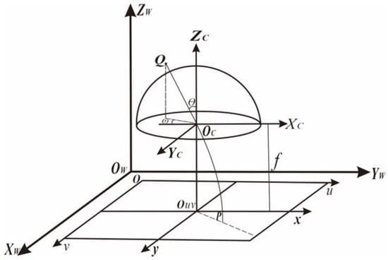
Figure 1.
Geometric model of fisheye camera imaging.
However, the deviation between the actual fisheye lens and the ideal spherical lens still exists; this deviation in the imaging plane is mainly expressed as an optical distortion and can be decomposed into radial distortion, eccentric distortion according to the distortion characteristics.
(1) The radial aberration difference is the radial displacement between the distorted image point and the theoretical image point, which is an axisymmetric distortion. The radial distortion model can be expressed as
where , and are the radial distortion parameters, is the distance from the fisheye image point to the center of the fisheye image and , represent the radial distortion in the u and v directions, respectively, represents the coordinates of the center of the fisheye image.
(2) The optical system of the center projection has varying degrees of decentered distortion, The reason for this distortion is mainly the optical axis of the lens, and the camera optical axis is not the axis. The decentered distortion model can be expressed as
where and are the decentered distortion parameters, represents the decentered distortion in the u and v directions.
Combining the two distortion models above together, the fisheye camera optical distortion model can be expressed as
where Δ and Δ represent the optical distortion in the u and v directions, , , , are the distortion parameters of the fisheye lens to be solved.
2.2. The Relationship between Spherical and Perspective Projection Model
The spherical projection model of a fisheye camera is shown in Figure 2. In order to describe its imaging process, a coordinate system is first established, where O-UV is the image coordinate system, assuming that there is a virtual image plane E tangent to the spherical surface of the fisheye head, and the point P is any point in space, and the point p′ is the projection point of the point P on the virtual image plane E with coordinates (u′, v′), which can be regarded as the perspective projection image point. The point p″ is the projection point of P on the fisheye image with coordinates (u, v).
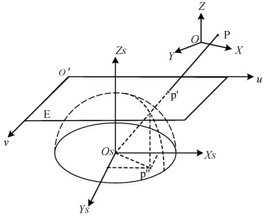
Figure 2.
Spherical projection with fisheye lens.
Four types of fisheye lens projection models are equal stereographic projection model, equidistant projection model, equisolid angle projection model, and orthographic projection model. The equidistant projection model, which is currently the most widely used fisheye lens imaging model, is expressed by
where and θ are the focal distance and angle of incidence. Planar correction is the operation of removing aberrations from fisheye lens images so that the output image conforms to human visual habits. Specifically, the image without distortion is derived from the perspective image principle, that is, imaging on plane E. The relationship between p′ and p″ is easily obtained through geometric relations as
Substituting Equations (4) and (5) into Equation (6), we have
where , , and are the number of pixels per millimeter in the direction and direction, respectively.
With Equation (6), the relationship between the image point coordinates on the fisheye image, and the image point coordinates on the perspective image can be established.
2.3. Orthorectification Model for Fisheye Image
By using Equation (6) as an intermediate equation, the relationship between the fisheye image and the ortho-image can be established. Assume that the fisheye image point p (u, v) corresponds to the corrected DOM point P (U, V). Starting from the DOM point P, the corresponding image point p on the fisheye image corresponding to point P is inverted according to the IOPs, EOPs, and camera distortion of the image film and the elevation of point P. Since the calculation result of coordinates is not necessarily an integer when finding the corresponding image point p on the fisheye image, gray interpolation is performed, and then the gray value of the interpolated point p is assigned to the point P on the DOM. As shown in Figure 3, a schematic diagram of the orthorectified model of the fisheye image, the following equation can be derived from the three-point co-linearity of P-p′-Os in Figure 3.
where is the camera center position, are the orientation parameters, are the 9 parameters of the rotation matrix.
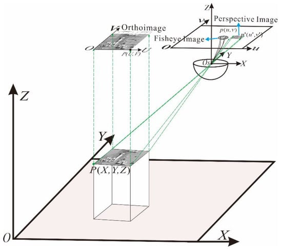
Figure 3.
Orthorectification model of fisheye image.
Substituting Equation (6) into Equation (7), we have
Since the optical aberration in the imaging process of the fisheye camera usually happens, the distortion is reflected in the fisheye image point coordinates. For this reason, in order to be more in line with the reality, the camera distortion (Equation (3)) is merged into Equation (8) to correct the fisheye image point coordinates, and the following formula is obtained.
From Equation (9), the expression of fisheye image point can be obtained.
Equation (10) is the fisheye image orthorectification model. Solving Equation (10) determines the IOPs and EOPs, and any ground point can be put onto a predefined orthorectified plane [46]. Since this paper uses the point-by-point method of orthorectification, if we want to calculate the pixel coordinates of each point of the original fisheye image by Equation (10), we need the 3D coordinates of each point, so we need to introduce the DEM, which can calculate the pixel coordinates of each point on the original fisheye image, and then interpolate the calculated pixel points and assign the grayscale, and finally, we can obtain the DOM.
In order to perform orthorectification of fisheye images using the method proposed in this paper, the parameters in Equation (10) need to be solved first. To this end, Taylor’s formula is applied to linearize Equation (10) relative to distortion parameters and EOPs, i.e.,
where ~ represent the partial derivatives of the fisheye camera under the equidistant projection model, respectively, the constant terms are = u − (u), = v − (v).
Equation (11) can be expressed by a matrix form as
where matrix represents the corrections of the EOPs of the fisheye camera, matrix represents the corrections of the IOPs of the fisheye camera, and s represents the corrections of the distortion parameters of the fisheye camera.
When there are redundant observations, least square adjustment is applied to solve the parameters, i.e.,
There are 14 unknown parameters in the above equations. At least 14 equations are needed. Two observation equations can be established using a single ground control point (GCP). This means that at least 7 reasonably distributed 3D GCPs and the corresponding fisheye image points are needed. In addition, since the initial values given are generally coarse, the solutions need to be iterated until a given threshold is met.
2.4. Orthorectification Process for Fisheye Image
After the parameters are solved above, the pixel coordinates on the original fisheye image can be calculated according to Equation (10), and thus the DOM can be produced as follow.
First, a DEM with the same size as the DOM needs to be obtained. The coordinates of the four corner image points of the original image are measured, and the corresponding actual plane coordinates are calculated by
where,
The length and width of the DOMs are then calculated based on the resolution of the DEM.
Second, since the fisheye image is an approximately circular image, the coordinates of the four corner points must first be measured by transforming all the fisheye image pixel points into the corresponding perspective projection image points using Equation (6) and then taking the coordinates of the four corner points from the perspective projection image points. The size of the DOM is determined by the ground sampling distance (GSD). The DEM can be divided into a grid by the resolution size, each grid corresponds to a pixel on the DOM, and the coordinates in the lower left corner of the DOM are determined as the starting point, and the coordinates of the pixels corresponding to the original image are sent out at every interval of the set resolution for grayscale interpolation.
Finally, the gray assignment to the DOM is generated. Figure 4 shows the flow chart of orthorectification of the fisheye image.
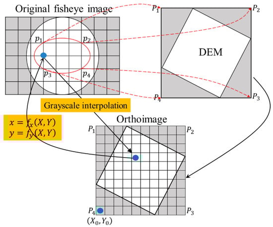
Figure 4.
Fisheye image orthorectification process.
3. Experiments and Analysis
3.1. Experiment 1
3.1.1. Indoor Calibration Field Set-Up
In order to verify the proposed method, an indoor calibration field is established to determine the relationship between the coordinates of image points on fisheye images and the corresponding 3D coordinates of spatial points. The dimension of the indoor calibration field is 6.5 m × 1.5 m × 4.0 m, with a three-layer steel frame structure. The distance between two adjacent steel frames is 0.75 m. An indium steel ruler is laid under the calibration field as a standard ruler for measurement (Figure 5a). In order to observe all the marked points as much as possible and reduce the measurement error, two stations with a height of 1.15 m were set up at 4.8 m in front of the left and 3.2 m in front of the right of the calibration site. The wall of the calibration site is white, with good lighting conditions, which enables multi-angle shooting at different heights and angles.
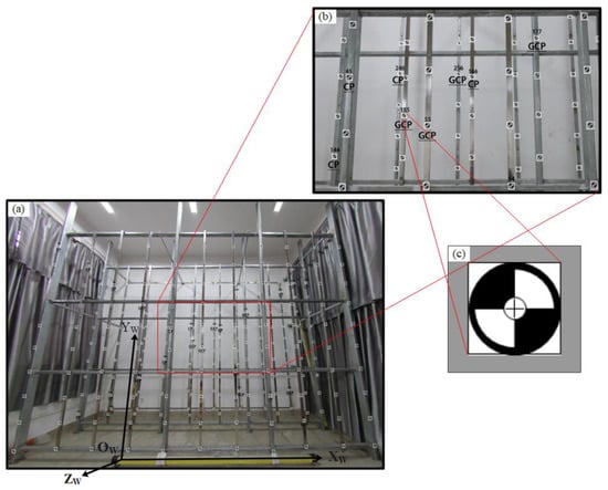
Figure 5.
The calibration field layout for Experiment 1: (a) The indoor calibration field; (b) The distribution diagram of GCPs; (c) The spy markers of the GCP.
There are 30 metal pillars in the calibration field, and the distance between two adjacent steel pillars is 0.75 m. Ten artificial marking points are evenly laid on each metal pillar, and a total of 300 artificial marking points are laid, which are evenly distributed on three planes (Figure 5b). In order to avoid mutual obscuration between the photographed marks, 110, 100, and 90 artificial marks were laid on the three planes. The layout of artificial marks meets the requirement that the number and distribution of marker points can be full and uniform. The spy marker is made of a 40 mm × 40 mm white square reflective sticker whose center is a black and white circle with a diameter of 40 mm. The center of the circle is made of precision cross wire whose width is 0.5 mm (Figure 5c). The spy marker is not only convenient for precision observation but also is conducive to extracting the center of the marker point in digital photos. The mark points are fixed on the pillar with strong adhesive to keep the relative position of the mark point stable for a long time. The flow chart of the orthorectification method is shown in Figure 6.
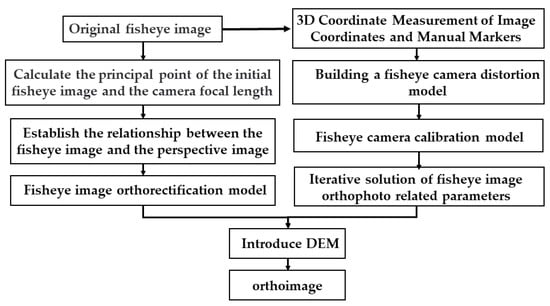
Figure 6.
The flow chart of the orthorectification method.
The steps of the manual marker measurement are as follows. Firstly, a free coordinate system is established, and the point O1 on the indium steel ruler is used as the origin of the free coordinate system, the direction O2O3 on the ruler is used as the X-axis, and the right-handed coordinate system is used. Set the coordinates of O1, O2 and O3 as (0, 0, 0), (1.79, 0, 0) and (2.82, 0, 0) respectively. Two Sokkia CX-102 total stations were set up at two sites (A and B). The horizontal and vertical angles of O1, O2, and O3 on the ruler were measured for eight rounds of the measuring process. The plane coordinates of the 2 GCPs (A and B) were determined using the rear intersection method. The elevations were obtained by using trigonometric leveling, and the 3D coordinates of the two survey sites (A and B) were solved.
30 GCPs were selected to measure their three-dimensional (3D) coordinates. To this end, two Sokkia CX-102 total stations were mounted on two stations (A and B), respectively, and used to measure the horizontal angle and vertical angle of each GCP. The plane coordinates of the GCPs were obtained by using the photogrammetric intersection method, and then the elevation was obtained according to the trigonometric leveling. By calculation, the three-dimensional coordinates of the GCPs were obtained. The accuracy of the intersection point of GCPs is calculated by [47]
where and represent the angle measurement errors at points respectively, and represent the horizontal distance between the points and GCP, represents the horizontal distance between and , represents the intersection angle.
The trigonometric leveling error of the GCPs derived from the error propagation is calculated by [47]
where is the RMSE of the distance between the measurement station and the point to be estimated, is the angle measurement error of the vertical angle, and α is the vertical angle.
Finally, by Equations (16) and (17), the average position accuracy of the calibration field is = 0.368 mm, and the average elevation accuracy is = 0.114 mm.
3.1.2. Fisheye Image I/EOPs and Distortion Parameters Solution
The photography is collected by a Canon 70D digital camera with a “CANON EF 8–15 mm f/4 L USM” fisheye lens with a FOV of 180°. The dimension of the original fisheye image is 3648 by 2432 pixels, and the theoretical pixel size of 6.16 µm (Figure 7a). The orthorectification program is coded in C++ language using the OPENCV4.5 library.
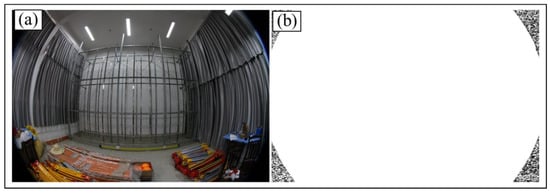
Figure 7.
Edge detection for the indoor calibration field image: (a) Original fisheye image; (b)Fisheye image segmentation result.
In order to obtain the initial value more accurately, the contour of the fisheye camera image is first segmented. Since the aspect ratio of the camera is not necessarily a 1:1 relationship, the contour of the fisheye image is considered to be a nearly circular ellipse. Figure 7a demonstrates that the original fisheye image is curve-fitted, and the noise is removed. Figure 7b is the result of the segmented fisheye image.
The general expression for the ellipse equation is expressed by
The center of the ellipse is calculated by
where is the length of a single pixel of the fisheye image, is the width of a single pixel of the fisheye image.
The long semiaxis of the ellipse is calculated by
The short semiaxis of the ellipse is calculated by
The principal distance is calculated by
After image segmentation, 200 edge points of the fisheye image were extracted for fitting calculation, and the centers and radii of the two images were estimated according to the curve equation (Equation (18)). By solving the coefficients () of the curve equation, we obtained the center coordinates of the ellipse and the long semiaxis () and short semiaxis () by Equations (19)–(21).
In general, the accuracy of this calibration model depends on the number and location of the selected GCPs. After calculation, the IOPs are = 1805.8 pixels, = 1210.3 pixels, = 1329.2 pixels. The result of the above calculation is used as the initial IOPs, the average 3D coordinates of the GCPs is used as the initial value of the photographic center position, and the initial angular orientation, as well as the distortion parameter, is 0.0. By using the initial calculated values and the 3D coordinates of the nine control points on the indoor calibration field and their corresponding fisheye image point coordinates, the fisheye image point error equation (Equation (12)) is solved iteratively. Table 1 shows the exact solutions of the 14 unknown parameters after adjustment calculation.

Table 1.
The calibration results for the indoor calibration field.
3.1.3. Orthorectification of Fisheye Image and DOM Accuracy Evaluation
After the IOPs, EOPs and distortion parameters of the fisheye camera were obtained, the DOM is generated by the method proposed above, where the “DEM” of the calibration field was inputted. After transforming all the fisheye image pixel points and interpolating the grayscale, the DOM was produced, and the result is shown in Figure 8.
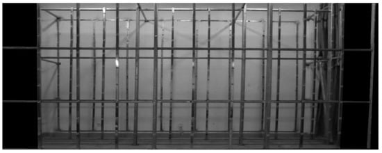
Figure 8.
The DOM generated by the method above for the indoor 3D calibration field.
In order to evaluate the accuracy of the DOM, a number of checkpoints (CPs) on the DOM were selected, and the coordinates of the CPs were compared with those of the measured CPs to obtain the RMSE. The RMSE along the X-direction is denoted as RMSx, along the Y-direction as , and the RMSE in the plane as . They are calculated by
where, is the coordinate of the ith CP on the DOM, is the actual measured coordinate of the CP, n is the number of CPs, and i is the CP number.
Table 2 shows the errors in the X-direction and Y-direction of the DOM of Experiment 1.
Table 2.
The plane accuracy in Experiment 1.
The first view DOM was evaluated for accuracy using 10 CPs. The average errors of DOM plane coordinates are 0.0026 m and 0.0017 m. It is calculated that the = 0.0027 m in the X direction, the = 0.002 m in the Y direction, and the = 0.003 m in the plane. The accuracy of the orthorectified image at 0.002 m resolution in the first view is better than three pixels.
3.2. Experiment 2
3.2.1. Outdoor Calibration Field Set-Up
In order to verify the proposed method, the outdoor calibration field is set up on the north wall of a building on the campus of Guilin University of Technology, China. The building is 28 m high and 80 m long. To meet the requirements of depth information for calibration experiments, it has a four-level concave and convex hierarchical structure, including grooves, walls, windows, columns, etc. The area around the site is relatively open, and the shooting distance is suitable.
After the site selection, the subsequent work was the placement of the calibration field control points. Since there are recesses and columns on the surface of the teaching building, it is difficult to paste control points on the teaching building, so we can only use the existing structures. In the wall of the building, 96 feature points that are not easily deformed were evenly selected as “GCPs” (Figure 9).
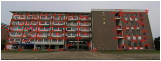
Figure 9.
The distribution diagram of GCPs for the outdoor calibration field.
Firstly, a free coordinate system was established, with the GCP (S1) as the origin, the vertical calibration field direction as Z-axis, the parallel to the wall direction as X-axis, and the plumb line as Y-axis. Two Sokkia CX-102 total station instruments were used respectively to obtain the spatial coordinates of the GCPs at two stations, and the average of the measurement results of the two stations was taken as the final result.
3.2.2. I/EOPs and Distortion Parameters for Fisheye Image
The experiments in the second experimental area used the same digital camera and fisheye lens as in the first experimental area.
Figure 10a is a fisheye image captured for the outdoor field. This image demonstrates that the original fisheye image is curve-fitted, and the noise is removed. Figure 10b is the result of the segmented fisheye image.
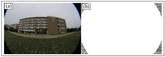
Figure 10.
Edge detection for the outdoor calibration field image: (a) Original fisheye image; (b) Fisheye image segmentation result.
After image segmentation, 200 edge points of the fisheye image were extracted for fitting calculation. The initial values were calculated as = 1802.2 pixels, = 1215.3 pixels, and = 1327.6 pixels. The IOPs, EOPs, and distortion parameters were iteratively calculated, and Table 3 is the result of the final calibration.
Table 3.
The calibration results for the outdoor calibration field.
3.2.3. Orthorectification of Fisheye Image and DOM Accuracy Evaluation
After the IOPs, EOPs and distortion parameters of the fisheye camera were obtained, the DOM of the fisheye image in Experiment 2 was generated by the method proposed above, where the “DEM” of the calibration field was inputted. After transforming all the fisheye image pixel points and interpolating the grayscale, the DOM was produced and the result is shown in Figure 11.
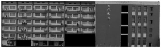
Figure 11.
The generated DOM for the outdoor calibration field.
Table 4 shows the errors in the X-direction and Y-direction of the DOM of the fisheye image for experiment 2.
Table 4.
The plane accuracy in experiment 2.
The second view DOM was evaluated for accuracy using nine GCPs. The average errors of DOM plane coordinates are 0.096 m and 0.151 m. It is calculated that the = 0.22 m in the X direction, the = 0.19 m in the Y direction, the = 0.29 m in the plane. The accuracy of the second view at 0.1 m resolution DOM is better than three pixels.
3.3. Experiment 3
3.3.1. Ground Calibration Field Set-Up
In order to verify the proposed method, the ground calibration field is selected to be located in the school library square. The area of the ground calibration field is 0.2 km × 0.2 km. There are a variety of ground objects in the calibration site, and the maximum height difference is 30 m, which meets the depth information required by the camera calibration (Figure 12a).
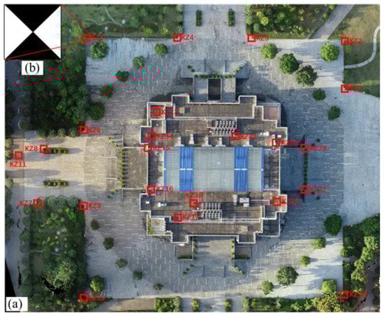
Figure 12.
The calibration field layout for Experiment 3: (a) The ground calibration field; (b) The GCP target in the ground calibration field.
For the layout of ground control points, the main factors to be considered include the size, number, distribution, and accuracy of GCPs. In order to meet the 1:2000 large-scale mapping, the flight height is designed at 100–200 m. Meanwhile, fully considering the actual needs of the aerial photography task of the light and small unmanned aerial vehicle (UAV), the size of the GCP target in the ground calibration field is designed to be 30 cm × 30 cm, whose shape is composed of two diagonal triangles (Figure 12b).
The GCP coordinates were measured by “Goodsurvey H6C” real-time kinematic (RTK), which used RTK reference station + mobile station smoothing mode. The coordinates are referenced to CGCS2000 coordinate system, and the elevation is in geodetic height.
3.3.2. Fisheye Image I/EOPs and Distortion Parameters Solution
The aerial photography experiment used a “DJI Mavic air2” UAV with a special fisheye lens with a 180° FOV. The image sensor size is 1/2 inch, and the dimension of the original fisheye image is 4000 by 2250 pixels.
Figure 13a is a fisheye image captured for the ground calibration field, which demonstrates that the original fisheye image is curve-fitted, and the noise is removed. Figure 13b is the result of the segmented fisheye image.
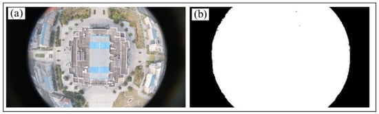
Figure 13.
Edge detection for the ground calibration field image: (a) Original fisheye image; (b) Fisheye image segmentation result.
After image segmentation, 200 edge points of the fisheye image were extracted for fitting calculation. The initial values were calculated as = 2044.2 pixels, = 1169.8 pixels, and = 987.8 pixels. The IOPs, EOPs, and distortion parameters were iteratively calculated, and Table 5 is the result of the final calibration.
Table 5.
The calibration result for the ground calibration field.
3.3.3. Orthorectification and Accuracy Evaluation
After the IOPs, EOPs, and distortion parameters of the fisheye camera were obtained, the DOM is generated by the method proposed, where the “DEM” of the calibration field was inputted. After transforming all the fisheye image pixel points and interpolating the grayscale, the DOM was produced. The result is shown in Figure 14.
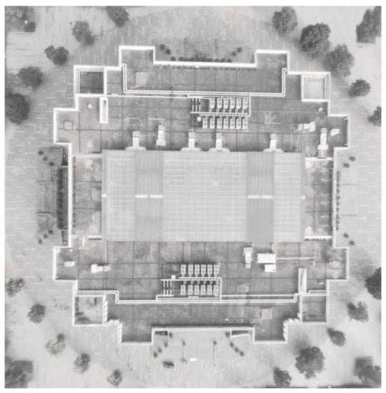
Figure 14.
The generated DOM for the ground calibration field.
Table 6 shows the errors in the X-direction and Y-direction of the DOM of Experiment 3.
Table 6.
The plane accuracy in Experiment 3.
The third view DOM was evaluated for accuracy using 13 GCPs. It is calculated that the = 0.428 m in the X-direction and = 0.434 m in the Y-direction, and the error in the X-direction is better than the error in the Y-direction. The = 0.610 m in the plane. The maximum absolute values of X and Y coordinates are 0.664 m and 0.645 m, respectively, and the minimum values are 0.112 m and 0.148 m, respectively. The accuracy of the 0.1 m resolution DOM in the third view is better than seven pixels.
4. Discussion
The fish-eye lens camera offers the characteristics of efficient acquisition of image data with serious distortions due to its wide field of view. The correction method in this paper solves the problem that the fisheye image has serious distortions and cannot meet the requirement of accurate measurement. Our method is suitable for indoor and outdoor environments. However, there are deficiencies in the research and errors in the DOM, for which the DEM is introduced, and a fisheye image orthorectification model based on an equidistant projection model is proposed.
4.1. Error Analysis of the DOM
By evaluating the plane accuracy of the DOM, it discovers that the orthorectification method proposed in this paper can meet the requirements in practical applications. However, there are still errors in the DOM, which are caused by that
- (1).
- Although the calibration field of the fish-eye camera is established, and the strict calibration model and the adjustment method are presented in this paper, the measurement of the coordinates of the CPs is greatly affected by the limitations of measuring instruments and measurement environment, resulting in the inaccuracy of the calibration results of the fish-eye camera.
- (2).
- The DEM or digital surface model with error, which is used for DOM generation, is propagated to DOM, resulting in DOM error.
- (3).
- The error is caused by inaccurate GCP position during extraction, since the distortion of a fisheye image is nonlinear, which is very difficult to be modeled, resulting in residuals.
4.2. Deficiencies in the Research
The correction model proposed in this paper can effectively and accurately correct fisheye camera images. However, there are still somewhat deficiencies. When the fisheye camera image is orthorectified, the edge of the fisheye image is vague, and the spatial information of an entire image cannot be fully utilized, resulting in that the margins of an image cannot be completely corrected.
In addition, the experimental area used for verification in this paper is small; a complex landform area with high buildings may be applied for verification in the near future.
5. Conclusions
All the theoretical basis in photogrammetry is based on the perspective projection of ordinary aerial cameras, whose field of view is generally less than 90°. With the fisheye camera’s field of view close to or even more than 180°, the image obtained by the fisheye camera does not follow up the perspective projection. Moreover, the fisheye camera image contains serious aberrations, resulting in the accuracy of the orthorectified image (called DOM) cannot meet the requirement. This paper firstly determines the transformation relationship between the fisheye image points and the perspective projection points according to the equidistant projection model, i.e., determines the spherical distortion of the fisheye image; then introduces the transformation relationship and the fisheye camera distortion model into the collinearity equation to derive the fisheye image orthorectification model. In addition, in order to calibrate the fisheye camera, a three-dimensional calibration field is established in this study, and its IOPs, EOPs, and optical distortion parameters are obtained by the proposed calibration model.
Three experiments are conducted to verify the method proposed in this paper. The experimental results demonstrate that the method can effectively correct the fisheye camera images into DOMs, and the RMSE of the first DOM is 0.0027 m in the X-direction, 0.002 m in the Y-direction, and 0.003 m in the plane; the RMSE of the second DOM is 0.22 m in the X-direction, 0.19 m in the Y-direction, and 0.29 m in the plane; the RMSE of the third DOM is 0.4425 m in the X-direction, 0.4206 m in the Y-direction, and 0.6105 m in the plane.
Author Contributions
Conceptualization, G.Z., B.S. and H.L.; methodology, H.L. and R.S.; software, G.Z. and Q.W.; validation, R.S. and Q.W.; formal analysis, H.L.; investigation, G.Z. and J.X.; resources, G.Z. and H.L.; data curation, G.Z. and B.S.; writing—original draft preparation, H.L. and R.S.; writing—review and editing, G.Z.; visualization, G.Z.; supervision, R.S.; project administration, G.Z.; funding acquisition, G.Z. All authors have read and agreed to the published version of the manuscript.
Funding
This paper is financially supported by the National Natural Science of China (the grants #: 41961065), Guangxi Natural Science Foundation for Innovation Research Team (the grant #: 2019GXNSFGA245001), the Guangxi Innovative Development Grand Program (the grant #: Guike AD19254002), and the BaGuiScholars program of Guangxi.
Conflicts of Interest
The authors declare no conflict of interest.
References
- Zhou, G.; Schickler, W.; Thorpe, A.; Song, P.; Chen, W.; Song, C. True orthoimage generation in urban areas with very tall buildings. Int. J. Remote Sens. 2004, 25, 5163–5180. [Google Scholar] [CrossRef]
- Zhou, G.; Yue, T.; Shi, Y.; Zhang, R.; Huang, J. Second-Order Polynomial Equation-Based Block Adjustment for Orthorectification of DISP Imagery. Remote Sens. 2016, 8, 680. [Google Scholar] [CrossRef]
- Wang, Q.; Zhou, G.; Song, R.; Xie, Y.; Luo, M.; Yue, T. Continuous space ant colony algorithm for automatic selection of orthophoto mosaic seamline network. ISPRS J. Photogramm. Remote Sens. 2022, 186, 201–217. [Google Scholar] [CrossRef]
- Zhou, G.; Zhang, R.; Liu, N.; Huang, J.; Zhou, X. On-Board Ortho-Rectification for Images Based on an FPGA. Remote Sens. 2017, 9, 874. [Google Scholar] [CrossRef]
- Zhou, G.; Chen, W.; Kelmelis, J.A.; Zhang, D. A comprehensive study on urban true orthorectification. IEEE Trans. Geosci. Remote Sens. 2005, 43, 2138–2147. [Google Scholar] [CrossRef]
- Zhou, G. Urban High-Resolution Remote Sensing:Algorithms and Modeling; CRC Press: Boca Raton, FL, USA, 2021. [Google Scholar] [CrossRef]
- Moreau, J.; Ambellouis, S.; Ruichek, Y. Fisheye-Based Method for GPS Localization Improvement in Unknown Semi-Obstructed Areas. Sensors 2017, 17, 119. [Google Scholar] [CrossRef]
- Courbon, J.; Mezouar, Y.; Martinet, P. Evaluation of the Unified Model of the Sphere for Fisheye Cameras in Robotic Applications. Adv. Robot. 2012, 26, 947–967. [Google Scholar] [CrossRef]
- Kim, D.; Choi, J.; Yoo, H.; Yang, U.; Sohn, K. Rear obstacle detection system with fisheye stereo camera using HCT. Expert Syst. Appl. 2015, 42, 6295–6305. [Google Scholar] [CrossRef]
- Li, T.; Tong, G.; Tang, H.; Li, B.; Chen, B. FisheyeDet: A Self-Study and Contour-Based Object Detector in Fisheye Images. IEEE Access 2020, 8, 71739–71751. [Google Scholar] [CrossRef]
- Kim, S.; Park, S.-Y. Expandable Spherical Projection and Feature Concatenation Methods for Real-Time Road Object Detection Using Fisheye Image. Appl. Sci. 2022, 12, 2403. [Google Scholar] [CrossRef]
- Yang, C.-Y.; Chen, H.H. Efficient Face Detection in the Fisheye Image Domain. IEEE Trans. Image Process. 2021, 30, 5641–5651. [Google Scholar] [CrossRef] [PubMed]
- Kokka, A.; Pulli, T.; Poikonen, T.; Askola, J.; Ikonen, E. Fisheye camera method for spatial non-uniformity corrections in luminous flux measurements with integrating spheres. Metrologia 2017, 54, 577–583. [Google Scholar] [CrossRef][Green Version]
- Lee, G.J.; Nam, W.I.; Song, Y.M. Robustness of an artificially tailored fisheye imaging system with a curvilinear image surface. Opt. Laser Technol. 2017, 96, 50–57. [Google Scholar] [CrossRef]
- Berveglieri, A.; Tommaselli, A.; Liang, X.; Honkavaara, E. Photogrammetric measurement of tree stems from vertical fisheye images. Scand. J. For. Res. 2017, 32, 737–747. [Google Scholar] [CrossRef]
- Feilong, L.; Erxue, C. Leaf AreaIndex Estimationfor QinghaiSpruceForest Using DigitalHemisphericalPhotography. Adv. Sci. 2009, 24, 803–809. [Google Scholar] [CrossRef]
- Zhou, G. Near Real-Time Orthorectification and Mosaic of Small UAV Video Flow for Time-Critical Event Response. IEEE Trans. Geosci. Remote Sens. 2009, 47, 739–747. [Google Scholar] [CrossRef]
- Zhou, G.; Jiang, L.; Huang, J.; Zhang, R.; Liu, D.; Zhou, X.; Baysal, O. FPGA-Based On-Board Geometric Calibration for Linear CCD Array Sensors. Sensors 2018, 18, 1794. [Google Scholar] [CrossRef]
- Schwalbe, E. Geometric modelling and calibration of fisheye lens camera systems. In Proceedings of the 2nd Panoramic Photogrammetry Workshop, International Archives of Photogrammetry and Remote Sensing, Berlin, Germany, 24–25 February 2005; p. W8. [Google Scholar]
- Ahmad, A.; Xavier, J.; Santos-Victor, J.; Lima, P. 3D to 2D bijection for spherical objects under equidistant fisheye projection. Comput. Vis. Image Underst. 2014, 125, 172–183. [Google Scholar] [CrossRef]
- Tommaselli, A.M.G.; Marcato, J., Jr.; Moraes, M.V.A.; Silva, S.L.A.; Artero, A.O. Calibration of panoramic cameras with coded targets and a 3d calibration field. ISPRS Int. Arch. Photogramm. Remote Sens. Spat. Inf. Sci. 2014, XL-3/W1, 137–142. [Google Scholar] [CrossRef]
- Sahin, C. Comparison and calibration of mobile phone fisheye lens and regular fisheye lens via equidistant model. J. Sens. 2016, 2016, 1–11. [Google Scholar] [CrossRef]
- Urquhart, B.; Kurtz, B.; Kleissl, J. Sky camera geometric calibration using solar observations. Atmos. Meas. Tech. 2016, 9, 4279–4294. [Google Scholar] [CrossRef]
- Zhang, Z. A flexible new technique for camera calibration. IEEE Trans. Pattern Anal. Mach. Intell. 2000, 22, 1330–1334. [Google Scholar] [CrossRef]
- Kannala, J.; Brandt, S.S. A generic camera model and calibration method for conventional, wide-angle, and fish-eye lenses. IEEE Trans. Pattern Anal. Mach. Intell. 2006, 28, 1335–1340. [Google Scholar] [CrossRef] [PubMed]
- Kanatani, K. Calibration of ultrawide fisheye lens cameras by eigenvalue minimization. IEEE Trans. Pattern Anal. Mach. Intell. 2012, 35, 813–822. [Google Scholar] [CrossRef]
- Arfaoui, A.; Thibault, S. Fisheye lens calibration using virtual grid. Appl. Opt. 2013, 52, 2577–2583. [Google Scholar] [CrossRef]
- Zhu, H.; Zhang, F.; Zhou, J.; Wang, J.; Wang, X.J.; Wang, X. Estimation of fisheye camera external parameter based on second-order cone programming. IET Comput. Vis. 2016, 10, 415–424. [Google Scholar] [CrossRef]
- Meng, L.; Li, Y.; Wang, Q.L. A Calibration Method for Mobile Omnidirectional Vision Based on Structured Light. IEEE Sens. J. 2020, 21, 11451–11460. [Google Scholar] [CrossRef]
- Hartley, R.; Kang, S.B. Parameter-free radial distortion correction with center of distortion estimation. IEEE Trans. Pattern Anal. Mach. Intell. 2007, 29, 1309–1321. [Google Scholar] [CrossRef]
- Schneider, D.; Schwalbe, E.; Maas, H.-G. Validation of geometric models for fisheye lenses. ISPRS J. Photogramm. Remote Sens. 2009, 64, 259–266. [Google Scholar] [CrossRef]
- Hughes, C.; McFeely, R.; Denny, P.; Glavin, M.; Jones, E. Equidistant (fθ) fish-eye perspective with application in distortion centre estimation. Image Vis. Comput. 2010, 28, 538–551. [Google Scholar] [CrossRef]
- Perfetti, L.; Polari, C.; Fassi, F. Fisheye photogrammetry: Tests and methodologies for the survey of narrow spaces. Int. Arch. Photogramm. Remote Sens. Spat. Inf. Sci. 2017, 42, 573–580. [Google Scholar] [CrossRef]
- Choi, K.H.; Kim, Y.; Kim, C. Analysis of fish-eye lens camera self-calibration. Sensors 2019, 19, 1218. [Google Scholar] [CrossRef] [PubMed]
- Kakani, V.; Kim, H.; Kumbham, M.; Park, D.; Jin, C.-B.; Nguyen, V.H. Feasible self-calibration of larger field-of-view (FOV) camera sensors for the advanced driver-assistance system (ADAS). Sensors 2019, 19, 3369. [Google Scholar] [CrossRef]
- Xu, Y.; Zhou, Q.; Gong, L.; Zhu, M.; Ding, X.; Teng, R.K. High-speed simultaneous image distortion correction transformations for a multicamera cylindrical panorama real-time video system using FPGA. IEEE Trans. Circuits Syst. Video Technol. 2013, 24, 1061–1069. [Google Scholar] [CrossRef]
- Lu, Y.; Wang, K.; Fan, G. Photometric calibration and image stitching for a large field of view multi-camera system. Sensors 2016, 16, 516. [Google Scholar] [CrossRef] [PubMed]
- Ying, X.-H.; Hu, Z.-Y. Fisheye lense distortion correction using spherical perspective projection constraint. Chin. J. Comput.-Chin. Ed. 2003, 26, 1702–1708. [Google Scholar]
- Si, W.; Yang, C. A fisheye image correction method based on longitude Model. Comput. Technol. Dev. 2014, 38–41, 46. [Google Scholar] [CrossRef]
- Zhao, K.; Liao, K.; Lin, C.; Liu, M.; Zhao, Y. Joint distortion rectification and super-resolution for self-driving scene perception. Neurocomputing 2021, 435, 176–185. [Google Scholar] [CrossRef]
- Yang, S.; Lin, C.; Liao, K.; Zhao, Y.; Liu, M. Unsupervised fisheye image correction through bidirectional loss with geometric prior. J. Vis. Commun. Image Represent. 2020, 66, 102692. [Google Scholar] [CrossRef]
- Zhao, K.; Lin, C.; Liao, K.; Yang, S.; Zhao, Y. Revisiting Radial Distortion Rectification in Polar-Coordinates: A New and Efficient Learning Perspective. IEEE Trans. Circuits Syst. Video Technol. 2022, 32, 3552–3560. [Google Scholar] [CrossRef]
- Liao, K.; Lin, C.; Zhao, Y.; Gabbouj, M. DR-GAN: Automatic radial distortion rectification using conditional GAN in real-time. IEEE Trans. Circuits Syst. Video Technol. 2019, 30, 725–733. [Google Scholar] [CrossRef]
- Zhou, G. Data Mining for Co-Location Patterns: Principles and Applications; CRC Press: Boca Raton, FL, USA, 2022. [Google Scholar] [CrossRef]
- Pi, Y.; Xin, L.; Chen, Z. Calibration and Rectification of Fisheye Images Based on Three-Dimensional Control Field. Acta Opt. Sin. 2017, 37, 11–15. [Google Scholar] [CrossRef]
- Zhou, G.; Xie, W.; Cheng, P. Orthoimage creation of extremely high buildings. IEEE Trans. Geosci. Remote Sens. 2008, 46, 4132–4141. [Google Scholar] [CrossRef]
- Department of Surveying Adjustment, School of Geodesy and Geomatics, Wuhan University. Error Theory and Foundation of Surveying Adjustment, 3rd ed.; Wuhan University Press: Wuhan, China, 2014; pp. 37–42. ISBN 978-7-307-12922-1. [Google Scholar]
Publisher’s Note: MDPI stays neutral with regard to jurisdictional claims in published maps and institutional affiliations. |
© 2022 by the authors. Licensee MDPI, Basel, Switzerland. This article is an open access article distributed under the terms and conditions of the Creative Commons Attribution (CC BY) license (https://creativecommons.org/licenses/by/4.0/).