Article

Integration of Photogrammetric and Spectral Techniques for Advanced Drone-Based Bathymetry Retrieval Using a Deep Learning Approach

by
Evangelos Alevizos
1,*,
Vassilis C. Nicodemou
2,
Alexandros Makris
2,
Iason Oikonomidis
2,
Anastasios Roussos
2 and
Dimitrios D. Alexakis
1
1
Laboratory of Geophysics—Satellite Remote Sensing & Archaeoenvironment (GeoSat ReSeArch Lab), Institute for Mediterranean Studies, Foundation for Research and Technology—Hellas (FORTH), Nikiforou Foka 130 & Melissinou, 74100 Rethymno, Crete, Greece
2
Computational Vision and Robotics Laboratory, Institute of Computer Science, Foundation for Research and Technology—Hellas (FORTH), N. Plastira 100, Vassilika Vouton, 70013 Heraklion, Crete, Greece
*
Author to whom correspondence should be addressed.
Remote Sens. 2022, 14(17), 4160; https://doi.org/10.3390/rs14174160
Submission received: 25 July 2022 / Revised: 16 August 2022 / Accepted: 21 August 2022 / Published: 24 August 2022
(This article belongs to the Special Issue Remote Sensing for Shallow and Deep Waters Mapping and Monitoring)

Abstract

:
Shallow bathymetry mapping using proximal sensing techniques is an active field of research that offers a new perspective in studying the seafloor. Drone-based imagery with centimeter resolution allows for bathymetry retrieval in unprecedented detail in areas with adequate water transparency. The majority of studies apply either spectral or photogrammetric techniques for deriving bathymetry from remotely sensed imagery. However, spectral methods require a certain amount of ground-truth depth data for model calibration, while photogrammetric methods cannot perform on texture-less seafloor types. The presented approach takes advantage of the interrelation of the two methods, in order to predict bathymetry in a more efficient way. Thus, we combine structure-from-motion (SfM) outputs along with band-ratios of radiometrically corrected drone images within a specially designed deep convolutional neural network (CNN) that outputs a reliable and robust bathymetry estimation. To achieve effective training of our deep learning system, we utilize interpolated uncrewed surface vehicle (USV) sonar measurements. We perform several predictions at three locations in the southern Mediterranean Sea, with varying seafloor types. Our results show low root-mean-square errors over all study areas (average RMSE ≅ 0.3 m), when the method was trained and tested on the same area each time. In addition, we obtain promising cross-validation performance across different study areas (average RMSE ≅ 0.9 m), which demonstrates the potential of our proposed approach in terms of generalization capabilities on unseen data. Furthermore, areas with mixed seafloor types are suitable for building a model that can be applied in similar locations where only drone data is available.

Graphical Abstract

1. Introduction

1.1. Optical Remote Sensing in Seafloor Mapping

Shallow seafloor bathymetry is an essential component in several coastal studies providing end users with valuable information about the underwater topography. Detailed shallow bathymetry data are required for a wide variety of applications, such as monitoring coastal erosion [1,2,3,4], and ecological mapping of benthic habitats [5,6,7]. However, the coastal seafloor has long been considered as a “white ribbon” [8], since traditional techniques such as sonar surveying are unable to provide full coverage at high spatial resolution (<1 m) in a time- and cost-effective way. Limiting factors such as the safe operational depth of the vessel and restricted sonar coverage due to survey geometry [9] hinder the quality and feasibility of high-resolution mapping in shallow areas. Other traditional topo-bathymetric surveying techniques, using total station or real-time kinematics (RTK) GPS stick, provide high precision data; however, they are not effective for covering large-scale shallow seafloor in detail.
Therefore, in recent years, there has been an increasing number of studies utilizing optical sensors for shallow seafloor mapping in areas with sufficient water transparency. These primarily include active optical sensors such as the light detection and ranging (LIDAR) systems as well as passive sensors (multi- or hyper-spectral) for a comprehensive retrieval of shallow bathymetry over large-scale areas. LIDAR datasets have been widely applied in shallow seafloor mapping studies due to their increased spatial resolution and data density along with their extensive coverage [10,11]. Particularly, airborne bathymetric LIDAR is the leading technology for studying nearshore bathymetry, providing meter-scale horizontal accuracy and centimeter-scale vertical accuracy over large areas of coastal seafloor [12,13]. However, the cost of LIDAR sensors and the costs and logistic effort for acquiring bathymetric LIDAR data are often limiting factors [14] that hinder the accessibility of this kind of technology to low-budget projects. On the other hand, space-borne or airborne passive optical sensors that record Earth’s surface radiance at different wavelengths (bands) have long been applied in deriving bathymetry [15,16,17,18]. This led to the development of a new technique, called satellite-derived bathymetry (SDB), which has now become a stand-alone discipline with numerous methods and applications. Satellite-derived bathymetry is achieved either by applying empirical formulas [17,18,19] tuned with ground-truth depth data or by using numerical techniques such as radiative transfer models [15,16,20]. The latter have the advantage of not requiring calibration data and they also provide an estimate of the total error of the final bathymetric product. However, empirical techniques are widely used since they do not require sophisticated software and they are simple to implement.

1.2. Satellite-Derived Bathymetry

Most of the empirical SDB techniques are based on the logarithmic band ratios approach introduced by [18] (see methods section), and lately there has been a tendency to combine machine learning techniques and empirical SDB algorithms. These novel approaches take advantage of the multi-dimensional nature of input datasets and have shown promising results. Ref. [21] applied an artificial neural network (ANN) approach on Landsat imagery showing promising results even for predicting depths greater than 20 m. Furthermore, Ref. [22] tested two ANN algorithms on IKONOS and Landsat imagery, which outperformed the optical modeling, and the regression trees techniques. Ref. [23] developed a new support vector machine (SVM) approach for deriving bathymetry using IKONOS-2 multispectral imagery. They performed training on a neighborhood scale and by using the full size of training dataset they obtained bathymetry with low (<1 m) RMSE values even for deeper waters (>16 m). Recently, Ref. [24] applied a convolutional neural network (CNN) technique on Sentinel-2 imagery, trained with sonar and LIDAR bathymetry for calculating SDB up to 15 m of water depth with 1-m error approximately.
A usual constraint in most empirical SDB studies is the requirement for comprehensive ground-truth depth measurements for tuning a regression model for bathymetry prediction. An additional constraint in empirical SDB studies, seafloor cover heterogeneity, which may induce depth inaccuracies in cases where the spectral difference due to seafloor cover is greater than the spectral difference due to depth [18]. This occurs particularly in shallow and relatively flat seafloor areas where mixed seafloor types (e.g., sand, reefs, algae, seagrasses) alternate spatially.

1.3. Structure from Motion

A technique that does not require ground-truth data input for deriving bathymetry from passive optical sensors is the application of photogrammetry along with multi-view satellite or aerial imagery [25,26]. Essentially, this approach takes advantage of image geometry and overlap along with image texture for producing a 3D surface from corresponding points between successive images. However, an important downturn of the method is that it requires seafloor surface with significant texture in order to provide useful outputs. In several cases, the seafloor occurs naturally featureless (e.g., flat with sediment cover), preventing the application of photogrammetric techniques. Additional requirements for successful photogrammetric results include accurate camera pose initialization (e.g., RTK accuracy), clear water, low wave height, minimal breaking waves, and minimal sun glint [27,28]. Light refraction due to the air–water interface is another potential issue that may be encountered during photogrammetric reconstruction of shallow seafloor. The reconstruction error caused by refraction directly depends on the water depth and on the incidence angles of the rays. High altitude flights allow reconstructions using only small incidence ray angles and therefore smaller refraction related errors. However, if rays with large incident angles are taken into account (e.g., to cover a larger area), the refraction error can remain significant even for high altitude flights which is also suggested by [29,30].
The latest advancements in Uncrewed Aerial Vehicle (UAV or drone) technology along with the development of structure from motion (SfM) techniques have paved the road for a new era in the field of geospatial disciplines [30]. Structure-from-motion (SfM) is one of the most applied photogrammetry techniques in studies using drone imagery. This technique has revolutionized the traditional photogrammetry method due to its efficacy to reconstruct 3D scenes without a priori knowledge of camera position [30]. Recent studies from [27,31] utilized drone-based imagery and SfM for deriving shallow water bathymetry in Mediterranean coastal areas under ideal sea-surface conditions. In order to correct for refraction, they trained a machine learning algorithm with LIDAR bathymetry using dense point clouds resulted from standard SfM, obtaining optimal results. In contrast, a similar study from [32] applied the refraction correction from [33] for reconstructing very shallow areas (<2 m) without significantly improving the final bathymetry. Another study that applies SfM for reconstructing shallow bathymetry is presented in [34]. In their study, the camera intrinsic and extrinsic calibration parameters were computed using frames from the onshore part of the dataset while refraction was corrected according to the method proposed in [35]. Similarly, Ref. [36] apply a multimedia bundle adjustment to account for refraction. They process initially images above land areas for deriving camera intrinsic and extrinsic parameters, and then they use these parameters as fixed during processing images from further offshore. Additionally, there have been a few recent studies applying empirical SDB (i.e., extensions of the logarithmic band-ratio technique) or analytical algorithms on drone-based multispectral imagery [28,37,38,39,40], showing good results with less than half a meter vertical errors. Particularly, Ref. [27] combined SfM and RGB color information in the same processing chain for bathymetry calculation. Initially, they performed 3D reconstruction in areas with rich seafloor texture, and then they applied the SfM outputs as inputs to machine learning models for optimizing bathymetry retrieval. Accordingly, Ref. [41] applied a deep learning methodology for extracting bathymetry by incorporating spectral and photogrammetric features of airborne imagery.

1.4. Aim of the Study

Considering the above-mentioned limitations of optical methods in deriving bathymetry, we propose a novel deep learning methodology tested on three study areas with contrasting seafloor types. This practice assists in evaluating better the proposed method under different scenarios of seafloor texture. Capitalizing on recent advancements in the field of machine learning, the presented study takes advantage of successful approaches in neural networks. The recent success of deep neural networks has led to the development of new tools, with improved performance compared to their predecessors. Specifically for image analysis, convolutional neural networks (CNNs) are the type of algorithms that are commonly used in literature [42,43,44,45] and have achieved important advances in diverse areas of image processing [45,46,47]. Therefore, we consider the application of CNN in this study in order to integrate the geometric and spectral approaches for optical bathymetry retrieval. This is the main novelty of the study, offering a new perspective in tackling the disadvantages of both methods when applied separately. In this way, we optimize the training process for bathymetry retrieval by minimizing the need for extensive ground-truth data input.
Initially, we develop an approximate 3D surface based on SfM over areas with textured seafloor and then combine it with spectral and spatial information for producing a final bathymetric output covering the entire area. This approach was tested over three study areas with diverse seafloor types for evaluating better its performance. In addition, we examine the influence of the amount of training data on the final bathymetry predictions and we assess the performance of each individually trained model (at each study area) by applying it to the remaining areas. In this way, we identify which areas are optimal for training a model that can be applied at a regional scale. The application of deep learning assists further in extracting maximum information from a diverse set of image datasets and thus achieves detailed bathymetry over any seafloor type. Ground-truth data collected with an Uncrewed Surface Vehicle (USV) are utilized for guiding the training process and validating the bathymetry predictions. This study exploits the versatility of uncrewed platforms (UAV and USV) along with state-of-the-art remote sensing techniques for accurate and detailed reconstruction of shallow bathymetry in a computationally efficient way and at low overall cost compared to other methods applied so far.

2. Methodology

2.1. Study Areas

The method was applied on the following three study areas, which have been selected according to the variability of seafloor cover and structure they present. All of the study areas comprise of waters with similar optical properties and have a Secchi depth greater than 10 m. These are characterized as optically transparent waters due to low concentrations of chlorophyll and suspended matter as a result of the oligotrophic character of eastern Mediterranean Sea [48] and the absence of significant input from adjacent drainage systems. The first study area is a small bay (Stavros) located at the north of Chania city (Crete, Greece, Figure 1). The seafloor captured by drone data is shallow in general reaching a maximum depth of 4 m and comprising of very smooth slope. The study area is generally homogeneous, covered partly with fine sand and partly with beach rock. The smooth bathymetry results in seafloor albedo, which changes gradually according to water depth. This provides an ideal case for studying the performance of both techniques in complementing each other. The second area (Kalamaki) is located a few kilometers west of Chania city (Figure 1). It comprises mainly of rough seafloor surface, made by rocky reefs, which are covered with various types of algae while there are also some shallow areas covered with fine sand. The maximum depth measured by the USV is 9 m and falls within the area covered by the drone images. The third area is located in the south-western coast of Crete (Elafonisi beach, Figure 1) and it also comprises of smooth seafloor, covered mainly with fine, foraminiferal sand and at places with submerged beach-rock and rocky reefs. The maximum depth recorded within the drone coverage area is −4.5 m. This site provides an additional setting for testing the effect of mixed seafloor types and repeatability of results. It has to be noted that, in the boundaries of Elafonisi and Stavros orthomosaics, the actual maximum depth might be 1–2 m deeper than the maximum recorded by the USV data. Thus, we have excluded these image parts from the prediction process in order to restrict the range of optimal bathymetry predictions within the range of the actual depth measurements.

2.2. Onshore Survey and Drone Platform Configuration

Prior to the drone surveys, a set of ground control points (GCPs) were measured along the coastline of each study area. The GCPs were measured with a real-time kinematics (RTK) GPS for achieving high accuracy (±2 cm). This level of accuracy is crucial in drone surveys that produce imagery with centimeter-scale spatial resolution while the onboard GPS sensor has a horizontal accuracy of approximately two meters. Thus, the GCPs are used for accurate orthorectification of the point-clouds and 2D reflectance mosaics. The drone platform comprises of a commercial DJI Phantom 4 Pro drone equipped with a 20 Mpixel RGB camera. The aerial survey data are presented in Table 1. By flying at an altitude of 120 m, it assists in minimizing the effect of: (a) air/water refraction and (b) image noise due to sun glint effects both on the sea-surface and on the seafloor (due to wave focusing). Drone imagery was processed with SfM techniques for producing an initial bathymetric surface (see following section). The raw imagery values were converted to reflectance by using a reference reflectance panel and Pix4D software (v4.5, Lausanne, Switzerland). The blue (B) and green (G) bands correspond to shorter wavelengths (460 ± 40 nm and 525 ± 50 nm respectively) and thus show deeper penetration through the water column [49]. The red (R) band corresponds to 590 ± 25 nm, which is highly absorbed in the first 1–2 m of water depth, but assists in emphasizing extremely shallow areas.

2.3. USV Surveys

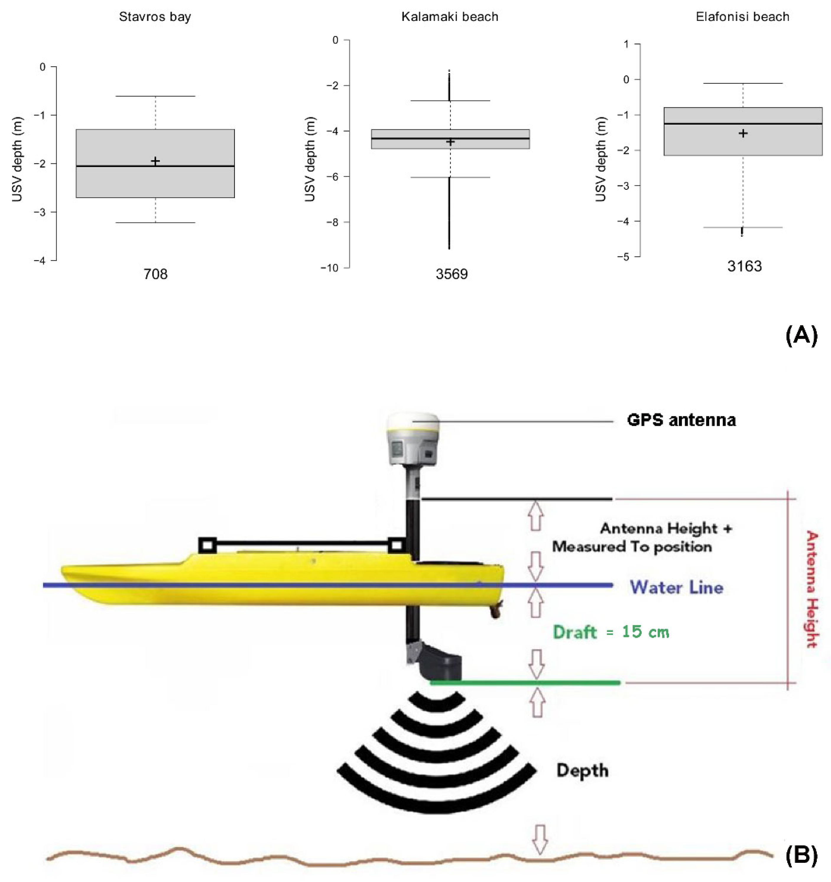
The diagram in Figure 2 shows the USV and sensors configuration. The USV used is a remote-controlled platform mounted with an Ohmex BTX single-beam sonar with an operating frequency of 235 kHz. The sonar is integrated with an RTK-GPS sensor and it collects attitude-corrected bathymetry points at 2 Hz sampling rate. The USV survey ground-truth bathymetry points are shown in Figure 2A. All USV data were collected on the same date with drone imagery in order to avoid temporal changes of bathymetry. The RTK-GPS measurements provide high spatial accuracy, which is essential in processing drone-based imagery with a pixel resolution of a few centimeters. At the Chania area, a total of 800 depth measurements were acquired, while at the Elafonisi area the USV survey yielded more than 3000 data points. Considering that the tidal range on the island of Crete is maximum ±0.2 m, and drone data acquisition has a one-hour difference with USV data, we infer that the tidal effect is completely negligible on the USV and drone data.

2.4. Structure from Motion

The OpenSfM open-source software was utilized for photogrammetric processing of the drone images [50]. The drone’s GPS and IMU data were used to initialize the camera extrinsic parameters. The intrinsic parameters were estimated during SfM using self-calibration. Given the very low ratio between the average water depth and the flight altitude, and the nadiral view of imagery, we assume that refraction effects are minimal and thus did not account for. The resulting 3D surface was not very accurate over smooth (feature-less) seafloor areas, and thus it was interpolated and used as an explanatory variable. This way, it provided a useful approximation of seafloor relief for guiding the predictive model.

2.5. Data Pre-Processing

The photogrammetrically derived bathymetry is expected to have captured in detail only areas with rich seafloor texture, leaving areas with homogeneous seafloor un-reconstructed. Thus, an integrated approach with full-scene spectral data is required for compensating for this issue. This approach relies on the empirical SDB method of Ref. [18], which employs the logarithmic band ratios from multispectral data (Equation (1)). This method is characterized by straightforwardness and versatility regarding its various implementations, and thus, it has been applied successfully on several recent studies [23,51,52,53,54]. The main concept of this approach is that light attenuation in the water column is exponential for wavelengths in the visible spectrum.
The original formula relies on the logarithmic ratio of two spectral bands (wavelengths) and two empirically tuned factors (Equation (1)):
z = m 1 l n n R w λ i l n n R w λ j m 0
where Rw (λi,j) is the water column reflectance of optically shallow water recorded at wavelength λi nanometres (with i < j), m1 is a tuneable constant to scale the ratio to depth, n is a fixed constant for all areas, and m0 is the offset for a depth of 0 m (e.g., tidal offset). The fixed value of n is chosen arbitrarily in order to assure both that the logarithm will be positive under any condition and that the ratio will produce a linear response with depth.
The coefficients m1 and m0 are determined by a set of ground-truth depth measurements for calibrating a linear regression equation, which then can be applied for calculating bathymetry. In addition, it is expected that Equation (1) is better tuned when spectral bands with good correlation with water-depth are available [55]. In order to prepare the imagery for use with the CNN model, we applied radiometric corrections using proprietary software Pix4D©. These corrections are necessary for converting raw image data to meaningful reflectance values, which are useful in quantitative image analysis such as spectral mapping [49]. Particularly, Ref. [56] showed that radiometrically corrected drone RGB imagery shows improved correlation with water depth. Initially, the pixel values are compensated for sensor bias such as sensor black-level, sensitivity, gain and exposure settings, and lens vignette effects and then they are converted to radiance values (i.e., in units W/m2/sr/nm, meaning watts per square meter per steradian per nanometer). Following, the radiance values are converted to spectral reflectance for each band, by incorporating the information from the calibrated reflectance panel (CRP). Apart from radiometric corrections, Pix4D provided geometric calibration for radial lens distortion using the specific camera model provided by the manufacturer.

2.6. Convolutional Network Architecture and Training Set

The CNN model used in this study follows the stacked-hourglass architecture suggested by [57]. This type of model was especially designed to find dominant features in multichannel inputs [57]. The specific architecture that we adopt here, has been successful in estimating depth values from multichannel images of faces and hands [58,59], which is a problem that shares some similarities with the problem of predicting bathymetry. In contrast to other networks for depth estimation [60,61], this architecture is more lightweight since it deals with image patches instead of the entire large image as input. In the work of [59], it was determined that a number between four and six stacked hourglass modules provided optimal depth reconstructions. Based on this and further experimentations (Section 3.1), we decided to use six stacked-hourglass modules in this study.
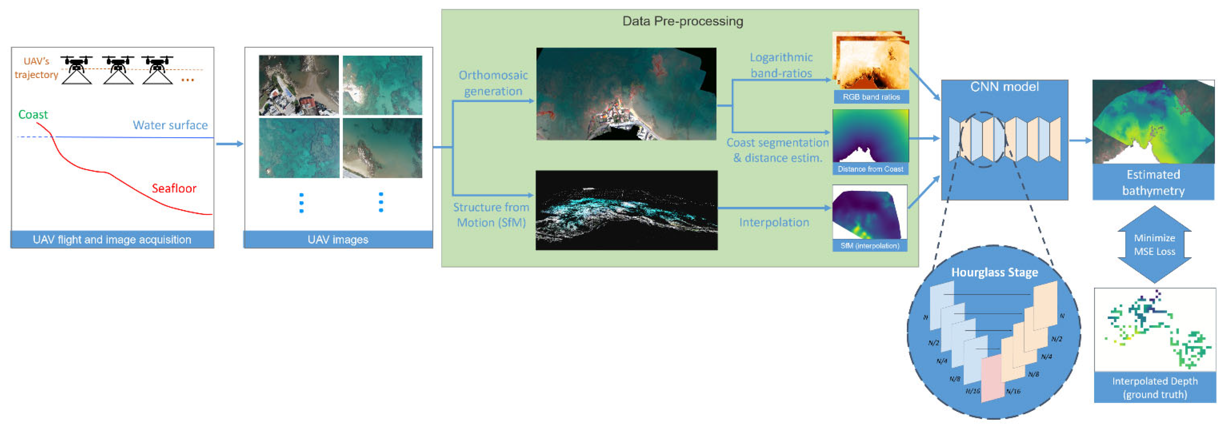
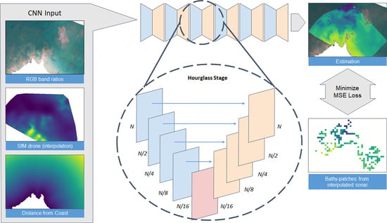
The training procedure of the CNN model is presented in Figure 3. First, an input traverses the network giving the network’s output. Next, the validity of the output is quantified with the loss function between the computed output and the defined ground-truth depth. The multichannel input of the CNN model consists of several image patches of size 128 × 128 pixels that includes five input rasters: three rasters for the logarithmic band-ratios (Blue/Green, Blue/Red and Green/Red), one for the approximate SfM surface, and one with the distance from coast information. In order to enhance the available geo-information of the training set, we decided to include the distance from coast for each pixel as an additional explanatory variable. Thus, we extracted the coastline by visual assessment of the RGB orthomosaics. The output of the training set (interpolated USV depth) consists of a 128 × 128 single channel image patch that depicts the depth values of the respective input, originating from the measurements of the USV. In the case of SfM and USV data, a thin-plate spline interpolation is applied within the region of each patch since the original data is composed of sparse measurements. Apart from the CNN model and for comparison purposes we also applied Random Forests (RFs) [62] and Support Vector Machines (SVM) [63] algorithms using a common training dataset from the Kalamaki area. RFs operate by aggregating the votes of several decision trees that each has been trained on predicting a particular parameter. Aggregation helps avoiding noise and extending the generalization capability of the resulting predictions. SVMs are based on the insight that, for a binary classifier, there is a decision boundary around which the classification prediction switches between the two classes. This boundary is essentially defined by the samples that are closest to each other and labeled of opposite class. Both approaches have been originally proposed as classifiers, and later extended for regression tasks.

3. Results

In this section, we present the results of our proposed method in the three study areas. We also include an ablation study to highlight the contribution of each component of our method. Furthermore, we compare it with previous deep learning approaches as well as with conventional machine learning methods (RFs, SVMs). Finally, we show the generalization capabilities of our method with a cross-validation experiment between all study areas.

3.1. Bathymetry Results on the Study Areas

To evaluate the performance of our method, we conducted three experiments on each study area, respectively. The experiments consist of a training and testing procedure on the respective train and test sets of each study area.
From all the patches that constitute a study area, we used a random subset of 60% of them for training, and the remaining 40% for testing. The training–test split of the data was based on the checkerboard block approach suggested by [64,65] as the most effective way to eliminate spatial autocorrelation effects during data validation. Furthermore, it is worth mentioning that, while the train/test patches are in several cases adjacent, we do not use the entire test patches in order to calculate the reported results. In fact, we use part of the USV points that are within the test patches: The USV points that are close (<3 m) to any train patch are discarded, leaving a smaller number of USV points, near the center of the test patch, to be used as ground-truth test depth values.
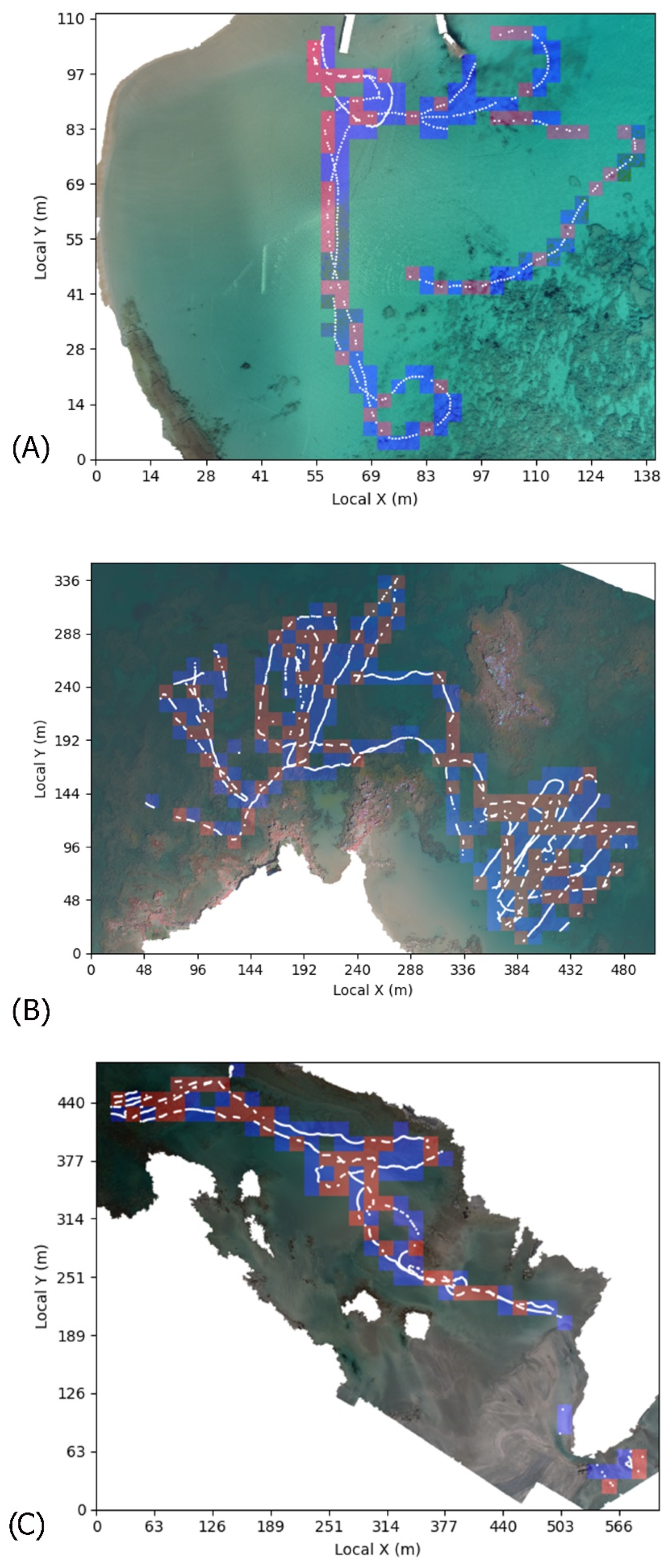
In Figure 4, we present a visualization example of the patches selected for training (in blue) and testing (in red) along the USV measurements (white dots) using the 60/40 training/testing ratio. The 60/40 data split was chosen as a more balanced scenario where the training set does not overwhelm the test set and thus highlights the CNN performance better. Particularly, regarding the Stavros bay, 94 patches were selected for training and 52 for testing; for the Kalamaki beach, 155 patches were selected for training and 107 for testing; and for the Elafonisi beach, 63 patches were selected for training and 45 for testing.
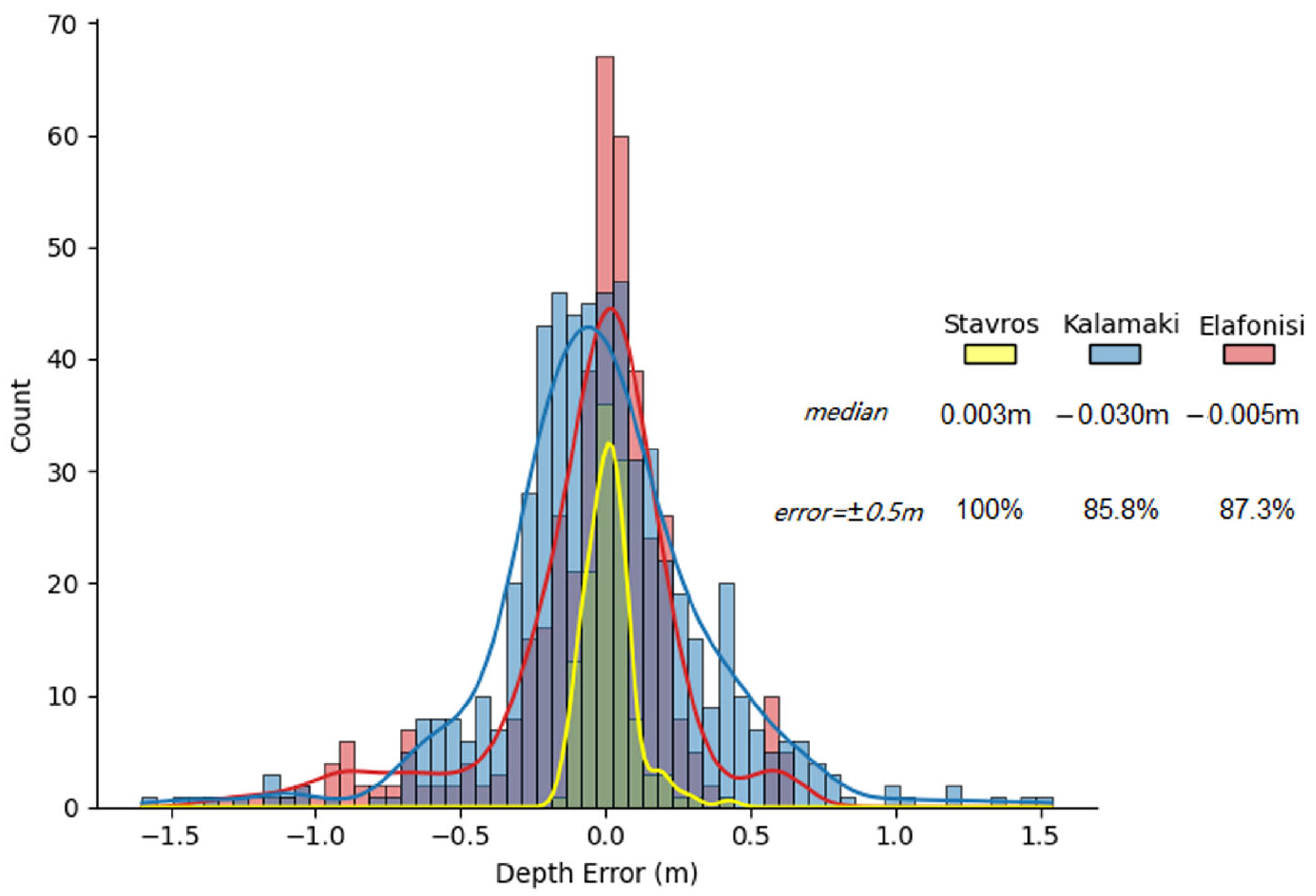
The test results of the three experiments are reported in Figure 5. The predicted bathymetry at the Stavros area (Figure 5A) shows maximum correlation with USV depth measurements despite a few artifacts in the middle of the scene. These artifacts are probably due to tiling effects on the reflectance mosaic. In addition, the RMSE value for the Stavros results is less than 10 cm. The predicted bathymetry at the Kalamaki area (Figure 5C) shows very good correlation with USV depth measurements and has an RMSE value of 35 cm. At the Elafonisi area, the predicted bathymetry (Figure 5E) shows very good correlation with USV depth measurements and has an RMSE value of 33 cm. The error distribution of the overall CNN predictions (Figure 6) suggests that each (local) model using 60% of the USV data for training, generalizes well the bathymetry beyond the training patches and over different seafloor types.

3.2. Ablation Study

In order to investigate the appropriate architecture choices and the optimal use of input data, we conducted a series of ablative experimentations to clarify these matters. The experiments’ aim is to show the advantage of using multiple stacks of hourglasses (as suggested by the literature), instead of using a single hourglass module. Moreover, the experiments justify the usage of the appropriate rasters (RGB band ratios, SfM, distance from coast) and their benefits towards estimation accuracy.
We trained variations of our model with the same training subset of Kalamaki beach and validated the choices on the respective test subset. The results reported in Table 2 indicate the beneficial use of multiple stacks compared to fewer stacks (single and triple hourglass). Furthermore, the results in Table 2 demonstrate the benefit of using multivariable input, as well as the ability of the network to handle it effectively, since only when we use all rasters jointly do we obtain the best results for bathymetry predictions.

3.3. Sensitivity Analysis of the Train–Test Split

Since the amount of our data is lower compared to other similar studies applying deep learning approaches, we analyze the sensitivity of our model to the amount of training/testing data, by applying different split ratios. Specifically, we used the 70/30, 60/40, 50/50, 40/60, and 30/70 training/testing ratios for each study area.
Table 3 shows how RMSE and R2 scores are influenced by the different ratio selection. These results suggest that the lower the training ratio, the higher the error of estimation is. This signifies that, despite the low total amount of data we have, the train/test sets are capable of describing the true behavior of our model.

3.4. Comparison with Artificial Neural Networks and Conventional Machine Learning Methods

Comparison of our CNN model with other ANN approaches cannot be achieved directly. The reason for that is mainly the lack of publicly available implementations that target specific problems of bathymetry estimation. Therefore, we try to approximate this comparison by creating the most well-known and commonly used ANN architecture. The case of a single stack hourglass is similar to the U-net type networks applied in previous bathymetry retrieval studies [41] using RGB or/and SfM as input. The output results shown in Table 2 demonstrate how this variant of networks is compared to our full stack model. Even though deep learning approaches have massive breakthroughs in many domains, conventional machine learning methods, such as random forests (RF) and support vector machines (SVM), manage to provide satisfactory results in shallow bathymetry mapping [66,67]. For that reason, we compared our CNN model with RF and SVM implementations using the same training and test set (60/40 split) of the Kalamaki area to train and test them. Specifically, an RF regression was used with 100 trees and a maximum tree depth = 8 and a Support Vector Regression with linear kernel, with C = 2.0 and parameter epsilon = 0.4 for the loss function.
The results in Table 4 show that the CNN model outperformed the commonly used machine learning algorithms and thus strengthened our motivation to apply it in this study.

3.5. Cross-Validation Study

In order to assess further the estimation capabilities of our approach, we conducted a cross-validation experiment between the three case studies. Specifically, we trained our CNN model on all patches (100% for training) of each study area and then we applied the model on the remaining two areas again for all their image patches. We repeated this procedure for all three cases, resulting in a 3 × 3 matrix as seen in Table 5. Table 5 reports the different RMSE values, each column corresponds to the case on which the model was trained, and each row corresponds to the case it was tested on. As expected, the diagonal of the matrix holds the lowest error values since the entire ground-truth set was used for training and testing thus providing artificially very low RMSE values. It is observed that data from Kalamaki beach provide the best training case when compared to the other areas, with an average RMSE of 0.8 m. This can be justified as this study area holds a greater variety of common features than the other two areas (rocky/featureless seafloors, and large coverage).

4. Discussion

4.1. Algorithm Performance

The results of the ablation study and the comparison with the RF and SVM methods (Table 2 and Table 4) assisted in framing better the performance of our CNN model among other machine learning approaches applied in earlier studies [41,66,67]. The CNN model yielded more accurate bathymetry predictions than the RF and SVM for the presented study areas and for the given amount of training/testing data. In addition, the ablation study using the full stack architecture provided a more successful model performance compared to the single and triple stack architecture that resembles the deep neural network applied by [41]. The combination of spectral (band-ratios), SfM and distance-to-coast rasters appear to explain bathymetry variability better than when a subset of those is used (Table 2). This evidence suggests that the proposed CNN model is a promising tool for extracting shallow bathymetry from drone imagery.
The CNN model applied in this study appeared to generalize well the training depth over a wider portion of each study area. Consequently, individual models predicted bathymetry over unknown seafloor with significant accuracy when they were trained with 60% of the ground-truth data. This led to at least 85% of bathymetry outputs having a low error value (<0.5 m, Figure 6). This suggests that sparse sonar measurements acquired with a USV provide sufficient training data for producing accurate bathymetry (RMSE < 0.4 m) over wider shallow areas such as bays and extended coastlines. Even when a smaller amount of training data is used, the output bathymetry accuracy does not decrease considerably, suggesting that the learning procedure is optimal and that each training set comprises of data representative of all seafloor types and depths. Only at the Elafonisi area, the R2 decreases enough when 40% of training data is used.
Technically, it required approximately two hours to train the model, while predicting took about 30 min on an Nvidia GeForce© GTX 1080 Ti GPUprocessor. The cross-validation results suggest that the CNN model, using the entire Kalamaki area data, provided the best overall accuracy (RMSE~0.8 m) when used for predicting the bathymetry in the other two study areas. This suggests that the CNN model of the Kalamaki area (100% of data for training) is more “regional” and thus relatively applicable in similar locations with small differences in seafloor types and water properties where additional ground-truth data are not available. This is probably explained by the fact that at the Kalamaki area more than 3500 interpolated depth measurements scattered over various seafloor types were used for training. It is suggested that a greater number of training data would further decrease the prediction error at the other two areas, as shown also by the experiments in Table 3.
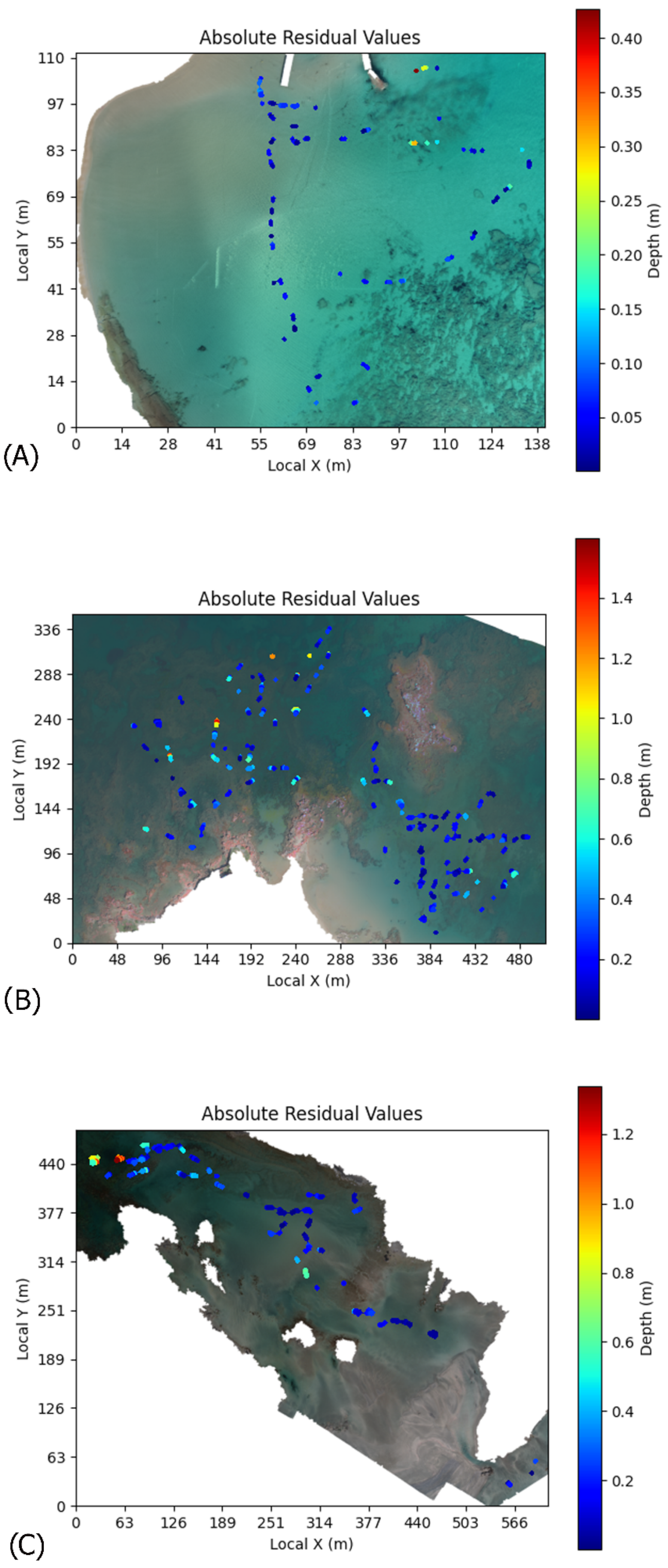
To assist better the evaluation of potential sources of error, Figure 7 shows the spatial distribution of residuals overlaid on RGB orthomosaics. Test points with large absolute value of residuals appear in a few instances over deep, rocky places of the Kalamaki and Elafonisi areas. A possible explanation could be that in rocky areas there are often dark or shaded parts of the seafloor, which may have led to erroneous bathymetric predictions. This issue was also encountered in the study of [37] where, similarly, large errors occurred over shaded patches in rocky areas. At the Stavros area, the few outliers that appear on the map are attributed to random noisy measurements, as the max absolute error values are generally low (0.4 m) compared to the other two areas.
The presented approach produces bathymetry predictions with low overall error for the given amount of training bathymetry data. Compared to other similar studies using drone-based imagery for empirical bathymetry retrieval [28,39], our approach achieves comparable errors; however, the main difference is that our training set is significantly more restricted than the one from Ref. [28], which is based on tens of thousands of points. Earlier SDB studies relied on abundant (several thousands) bathymetry data for training [22,23,67] using large training/test ratios. We consider that the efficacy of any empirical method in predicting bathymetry, should also consider the amount of training data required in order to achieve a particular accuracy level. In our case, the application of the USV platform assisted in obtaining targeted ground-truth depth measurements in a time- and cost-effective way. Thus, we utilized on average 1–2 thousands of depth measurements (60% scenario) in order to construct each of the training sets.

4.2. Future Considerations

In this study, we considered an alternative use of the SfM output surface and did not apply it as training output as in [28]. Instead, we produced small training patches by interpolating along the track of the USV point measurements. Interpolation of ground-truth data assists in data augmentation that is an essential procedure in deep model training. In contrast to more simple machine learning algorithms, which receive 1D point-based information, a CNN model requires 2D/3D data as training outputs. Therefore, data augmentation techniques are necessary for closing gaps in actual ground-truth data or even the explanatory variables [68]. In other words, a LIDAR or multi-beam sonar bathymetry dataset would be ideal for extracting training patches for the CNN. However, such data require significant cost and effort to be collected at shallow areas and thus fall beyond the concept of this study. The presented approach could be further benefited by specific improvements, which should focus on enhancing the quality of training datasets. Initially, it is recommended that for a successful SfM reconstruction, several environmental criteria should be met, such as textured seafloor, minimal sun glint, and nearly flat sea-surface. These conditions although challenging to be met simultaneously, they should greatly improve the SfM output and then it should be used for extracting suitable training patches for the CNN model. Furthermore, the USV application holds promising potential for producing 3D training patches from underwater imagery. The USV offers the possibility for collecting underwater images with considerable detail and texture up to a maximum depth depending on water clarity (for most Mediterranean coastal areas this depth should be between 5 to 10 m). This application would greatly enhance the capabilities of single-beam sonar by incorporating the RTK depth measurements into a SfM procedure similar to the one applied on drone images. An additional advantage of this application is that underwater images would be free from refraction artifacts. In this way, suitable bathymetric surfaces could be extracted and provide an improved source for training and testing the CNN model.

5. Conclusions

Hydrospatial datasets acquired with novel uncrewed platforms (drone, USV) show great potential in mapping shallow bathymetry in high resolution. The suggested deep learning approach combines the strengths of SfM and spectral methods simultaneously, resulting in a CNN model that predicts bathymetry with low error even when 60% of ground-truth data is used for training. This suggests that deep learning approaches result in an efficient use of input data, thus minimizing the cost and effort for data acquisition. The cross-validation tests showed that areas with mixed seafloor types are optimal for training a more “regional” CNN model that can be applied in unknown areas with similar water/seafloor types using only drone images. However, a greater amount of ground-truth data is required for achieving acceptable errors (<0.5 m) with the “regional” CNN model. Future work will focus on developing and testing a “regional” CNN model with better performance, and applying SfM on underwater imagery for increasing the capacity of training data in the deep learning procedure.

Author Contributions

Conceptualization, E.A.; data curation, E.A.; formal analysis, E.A., V.C.N., A.M. and I.O.; funding acquisition, A.R. and D.D.A.; investigation, I.O.; methodology, E.A., V.C.N., A.M. and I.O.; project administration, E.A., I.O., A.R. and D.D.A.; resources, I.O., A.R. and D.D.A.; software, V.C.N., A.M. and I.O.; supervision, A.R. and D.D.A.; validation, E.A., V.C.N., A.M., A.R. and D.D.A.; writing—original draft preparation, E.A., V.C.N. and A.M.; writing—review and editing, E.A., V.C.N., A.M., A.R. and D.D.A. All authors have read and agreed to the published version of the manuscript.

Funding

This research received funding from a 2020 FORTH-Synergy Grant.

Data Availability Statement

Data are available on request from the authors.

Acknowledgments

This study is part of the ACTYS project (https://actys.ims.forth.gr, accessed on 24 July 2022, Rethymno, Greece).

Conflicts of Interest

The authors declare no conflict of interest.

References

  1. Davidson, M.; Van Koningsveld, M.; de Kruif, A.; Rawson, J.; Holman, R.; Lamberti, A.; Medina, R.; Kroon, A.; Aarninkhof, S. The CoastView Project: Developing Video-Derived Coastal State Indicators in Support of Coastal Zone Management. Coast. Eng. 2007, 54, 463–475. [Google Scholar] [CrossRef]
  2. de Swart, H.E.; Zimmerman, J.T.F. Morphodynamics of Tidal Inlet Systems. Annu. Rev. Fluid Mech. 2009, 41, 203–229. [Google Scholar] [CrossRef]
  3. van Dongeren, A.; Plant, N.; Cohen, A.; Roelvink, D.; Haller, M.C.; Catalán, P. Beach Wizard: Nearshore Bathymetry Estimation through Assimilation of Model Computations and Remote Observations. Coast. Eng. 2008, 55, 1016–1027. [Google Scholar] [CrossRef]
  4. Janowski, L.; Wroblewski, R.; Rucinska, M.; Kubowicz-Grajewska, A.; Tysiac, P. Automatic Classification and Mapping of the Seabed Using Airborne LiDAR Bathymetry. Eng. Geol. 2022, 301, 106615. [Google Scholar] [CrossRef]
  5. Garcia, R.A.; Lee, Z.; Hochberg, E.J. Hyperspectral Shallow-Water Remote Sensing with an Enhanced Benthic Classifier. Remote Sens. 2018, 10, 147. [Google Scholar] [CrossRef]
  6. Kobryn, H.T.; Wouters, K.; Beckley, L.E.; Heege, T. Ningaloo Reef: Shallow Marine Habitats Mapped Using a Hyperspectral Sensor. PLoS ONE 2013, 8, e70105. [Google Scholar] [CrossRef]
  7. Purkis, S.J.; Gleason, A.C.R.; Purkis, C.R.; Dempsey, A.C.; Renaud, P.G.; Faisal, M.; Saul, S.; Kerr, J.M. High-Resolution Habitat and Bathymetry Maps for 65,000 Sq. Km of Earth’s Remotest Coral Reefs. Coral Reefs 2019, 38, 467–488. [Google Scholar] [CrossRef]
  8. Carvalho, R.C.; Hamylton, S.; Woodroffe, C.D. Filling the ‘White Ribbon’ in Temperate Australia: A Multi-Approach Method to Map the Terrestrial-Marine Interface. In Proceedings of the 2017 IEEE/OES Acoustics in Underwater Geosciences Symposium (RIO Acoustics), Rio de Janeiro, Brazil, 25–27 July 2017; pp. 1–5. [Google Scholar]
  9. Kenny, A.J.; Cato, I.; Desprez, M.; Fader, G.; Schüttenhelm, R.T.E.; Side, J. An Overview of Seabed-Mapping Technologies in the Context of Marine Habitat Classification. ICES J. Mar. Sci. 2003, 60, 411–418. [Google Scholar] [CrossRef]
  10. Costa, B.M.; Battista, T.A.; Pittman, S.J. Comparative Evaluation of Airborne LiDAR and Ship-Based Multibeam SoNAR Bathymetry and Intensity for Mapping Coral Reef Ecosystems. Remote Sens. Environ. 2009, 113, 1082–1100. [Google Scholar] [CrossRef]
  11. Taramelli, A.; Cappucci, S.; Valentini, E.; Rossi, L.; Lisi, I. Nearshore Sandbar Classification of Sabaudia (Italy) with LiDAR Data: The FHyL Approach. Remote Sens. 2020, 12, 1053. [Google Scholar] [CrossRef] [Green Version]
  12. Brock, J.C.; Purkis, S.J. The Emerging Role of Lidar Remote Sensing in Coastal Research and Resource Management. J. Coast. Res. 2009, 10053, 1–5. [Google Scholar] [CrossRef]
  13. Klemas, V. Beach Profiling and LIDAR Bathymetry: An Overview with Case Studies. J. Coast. Res. 2011, 277, 1019–1028. [Google Scholar] [CrossRef]
  14. Freire, R.; Pe’eri, S.; Madore, B.; Rzhanov, Y.; Alexander, L.; Parrish, C.; Lippmann, T. Monitoring Near-Shore Bathymetry Using a Multi-Image Satellite-Derived Bathymetry Approach; International Hydrographic Organization: National Harbor, MD, USA, 2015. [Google Scholar]
  15. Albert, A.; Mobley, C.D. An Analytical Model for Subsurface Irradiance and Remote Sensing Reflectance in Deep and Shallow Case-2 Waters. Opt. Express 2003, 11, 2873–2890. [Google Scholar] [CrossRef]
  16. Lee, Z.; Carder, K.L.; Mobley, C.D.; Steward, R.G.; Patch, J.S. Hyperspectral Remote Sensing for Shallow Waters: 2. Deriving Bottom Depths and Water Properties by Optimization. Appl. Opt. 1999, 38, 3831–3843. [Google Scholar] [CrossRef]
  17. Lyzenga, D.R. Passive Remote Sensing Techniques for Mapping Water Depth and Bottom Features. Appl. Opt. 1978, 17, 379–383. [Google Scholar] [CrossRef]
  18. Stumpf, R.P.; Holderied, K.; Sinclair, M. Determination of Water Depth with High-Resolution Satellite Imagery over Variable Bottom Types. Limnol. Oceanogr. 2003, 48, 547–556. [Google Scholar] [CrossRef]
  19. Lyzenga, D.R.; Malinas, N.P.; Tanis, F.J. Multispectral Bathymetry Using a Simple Physically Based Algorithm. IEEE Trans. Geosci. Remote Sens. 2006, 44, 2251–2259. [Google Scholar] [CrossRef]
  20. Dekker, A.G.; Phinn, S.R.; Anstee, J.; Bissett, P.; Brando, V.E.; Casey, B.; Fearns, P.; Hedley, J.; Klonowski, W.; Lee, Z.P.; et al. Intercomparison of Shallow Water Bathymetry, Hydro-Optics, and Benthos Mapping Techniques in Australian and Caribbean Coastal Environments. Limnol. Oceanogr. Methods 2011, 9, 396–425. [Google Scholar] [CrossRef]
  21. Gholamalifard, M.; Kutser, T.; Esmaili-Sari, A.; Abkar, A.A.; Naimi, B. Remotely Sensed Empirical Modeling of Bathymetry in the Southeastern Caspian Sea. Remote Sens. 2013, 5, 2746–2762. [Google Scholar] [CrossRef]
  22. Liu, S.; Gao, Y.; Zheng, W.; Li, X. Performance of Two Neural Network Models in Bathymetry. Remote Sens. Lett. 2015, 6, 321–330. [Google Scholar] [CrossRef]
  23. Wang, L.; Liu, H.; Su, H.; Wang, J. Bathymetry Retrieval from Optical Images with Spatially Distributed Support Vector Machines. GISci. Remote Sens. 2019, 56, 323–337. [Google Scholar] [CrossRef]
  24. Lumban-Gaol, Y.A.; Ohori, K.A.; Peters, R.Y. Satellite-Derived Bathymetry Using Convolutional Neural Networks and Multispectral SENTINEL-2 Images. Int. Arch. Photogramm. Remote Sens. Spat. Inf. Sci. 2021, 43B3, 201–207. [Google Scholar] [CrossRef]
  25. Cao, B.; Fang, Y.; Jiang, Z.; Gao, L.; Hu, H. Shallow Water Bathymetry from WorldView-2 Stereo Imagery Using Two-Media Photogrammetry. Eur. J. Remote Sens. 2019, 52, 506–521. [Google Scholar] [CrossRef]
  26. Hodúl, M.; Bird, S.; Knudby, A.; Chénier, R. Satellite Derived Photogrammetric Bathymetry. ISPRS J. Photogramm. Remote Sens. 2018, 142, 268–277. [Google Scholar] [CrossRef]
  27. Agrafiotis, P.; Skarlatos, D.; Georgopoulos, A.; Karantzalos, K. Shallow water bathymetry mapping from UAV imagery based on machine learning. arXiv 2019, arXiv:1902.10733. [Google Scholar]
  28. Slocum, R.K.; Parrish, C.E.; Simpson, C.H. Combined Geometric-Radiometric and Neural Network Approach to Shallow Bathymetric Mapping with UAS Imagery. ISPRS J. Photogramm. Remote Sens. 2020, 169, 351–363. [Google Scholar] [CrossRef]
  29. Karara, H.M.; Adams, L.P. Non-Topographic Photogrammetry; American Society for Photogrammetry and Remote Sensing: Falls Church, VA, USA, 1989; ISBN 978-0-94442-610-4. [Google Scholar]
  30. Westoby, M.J.; Brasington, J.; Glasser, N.F.; Hambrey, M.J.; Reynolds, J.M. ‘Structure-from-Motion’ Photogrammetry: A Low-Cost, Effective Tool for Geoscience Applications. Geomorphology 2012, 179, 300–314. [Google Scholar] [CrossRef]
  31. Agrafiotis, P.; Karantzalos, K.; Georgopoulos, A.; Skarlatos, D. Learning from Synthetic Data: Enhancing Refraction Correction Accuracy for Airborne Image-Based Bathymetric Mapping of Shallow Coastal Waters. PFG—J. Photogramm. Remote Sens. Geoinf. Sci. 2021, 89, 91–109. [Google Scholar] [CrossRef]
  32. David, C.G.; Kohl, N.; Casella, E.; Rovere, A.; Ballesteros, P.; Schlurmann, T. Structure-from-Motion on Shallow Reefs and Beaches: Potential and Limitations of Consumer-Grade Drones to Reconstruct Topography and Bathymetry. Coral Reefs 2021, 40, 835–851. [Google Scholar] [CrossRef]
  33. Dietrich, J.T. Bathymetric Structure-from-Motion: Extracting Shallow Stream Bathymetry from Multi-View Stereo Photogrammetry. Earth Surf. Process. Landf. 2017, 42, 355–364. [Google Scholar] [CrossRef]
  34. Mandlburger, G. A case study on through-water dense image matching. In Proceedings of the International Archives of the Photogrammetry, Remote Sensing and Spatial Information Sciences, Riva del Garda, Italy, 30 May 2018; Copernicus GmbH: Goettingen, Germany, 2018; Volume XLII-2, pp. 659–666. [Google Scholar]
  35. Wimmer, M. Comparison of Active and Passive Optical Methods for Mapping River Bathymetry. Ph.D. Thesis, Technische Universität Wien, Wien, Austria, 2016. [Google Scholar]
  36. Mulsow, C.; Kenner, R.; Bühler, Y.; Stoffel, A.; Maas, H.-G. Subaquatic digital elevation models from UAV-imagery. In Proceedings of the International Archives of the Photogrammetry, Remote Sensing and Spatial Information Sciences, Riva del Garda, Italy, 30 May 2018; Copernicus GmbH: Goettingen, Germany, 2018; Volume XLII-2, pp. 739–744. [Google Scholar]
  37. Alevizos, E.; Oikonomou, D.; Argyriou, A.V.; Alexakis, D.D. Fusion of Drone-Based RGB and Multi-Spectral Imagery for Shallow Water Bathymetry Inversion. Remote Sens. 2022, 14, 1127. [Google Scholar] [CrossRef]
  38. Parsons, M.; Bratanov, D.; Gaston, K.; Gonzalez, F. UAVs, Hyperspectral Remote Sensing, and Machine Learning Revolutionizing Reef Monitoring. Sensors 2018, 18, 2026. [Google Scholar] [CrossRef] [PubMed]
  39. Rossi, L.; Mammi, I.; Pelliccia, F. UAV-Derived Multispectral Bathymetry. Remote Sens. 2020, 12, 3897. [Google Scholar] [CrossRef]
  40. Starek, M.J.; Giessel, J. Fusion of Uas-Based Structure-from-Motion and Optical Inversion for Seamless Topo-Bathymetric Mapping. In Proceedings of the 2017 IEEE International Geoscience and Remote Sensing Symposium (IGARSS), Fort Worth, Texas, USA, 23–28 July 2017; IEEE: New York, NY, USA; pp. 2999–3002. [Google Scholar]
  41. Mandlburger, G.; Kölle, M.; Nübel, H.; Soergel, U. BathyNet: A Deep Neural Network for Water Depth Mapping from Multispectral Aerial Images. PFG—J. Photogramm. Remote Sens. Geoinformation Sci. 2021, 89, 71–89. [Google Scholar] [CrossRef]
  42. He, K.; Zhang, X.; Ren, S.; Sun, J. Deep Residual Learning for Image Recognition. In Proceedings of the 2016 IEEE Conference on Computer Vision and Pattern Recognition (CVPR), Las Vegas, NV, USA, 27–30 June 2016; IEEE: New York, NY, USA; pp. 770–778. [Google Scholar]
  43. Russakovsky, O.; Deng, J.; Su, H.; Krause, J.; Satheesh, S.; Ma, S.; Huang, Z.; Karpathy, A.; Khosla, A.; Bernstein, M.; et al. ImageNet Large Scale Visual Recognition Challenge. Int. J. Comput. Vis. 2015, 115, 211–252. [Google Scholar] [CrossRef]
  44. Simonyan, K.; Zisserman, A. Very Deep Convolutional Networks for Large-Scale Image Recognition. arXiv 2014, arXiv:1409.1556. [Google Scholar]
  45. Yao, G.; Lei, T.; Zhong, J. A Review of Convolutional-Neural-Network-Based Action Recognition. Pattern Recognit. Lett. 2019, 118, 14–22. [Google Scholar] [CrossRef]
  46. Chang, J.-R.; Chen, Y.-S. Pyramid Stereo Matching Network. In Proceedings of the 2018 IEEE/CVF Conference on Computer Vision and Pattern Recognition, Salt Lake City, UT, USA, 18–23 June 2018; IEEE: New York, NY, USA; pp. 5410–5418. [Google Scholar]
  47. Ronneberger, O.; Fischer, P.; Brox, T. U-Net: Convolutional Networks for Biomedical Image Segmentation. In Proceedings of the Medical Image Computing and Computer-Assisted Intervention—MICCAI 2015, Munich, Germany, 5–9 October 2015; Navab, N., Hornegger, J., Wells, W.M., Frangi, A.F., Eds.; Springer International Publishing: Cham, Switzerland, 2015; pp. 234–241. [Google Scholar]
  48. Ignatiades, L. The Productive and Optical Status of the Oligotrophic Waters of the Southern Aegean Sea (Cretan Sea), Eastern Mediterranean. J. Plankton Res. 1998, 20, 985–995. [Google Scholar] [CrossRef]
  49. Eugenio, F.; Marcello, J.; Martin, J.; Rodríguez-Esparragón, D. Benthic Habitat Mapping Using Multispectral High-Resolution Imagery: Evaluation of Shallow Water Atmospheric Correction Techniques. Sensors 2017, 17, 2639. [Google Scholar] [CrossRef]
  50. OpenSfM. 2022. Available online: https://opensfm.org (accessed on 10 January 2022).
  51. Geyman, E.C.; Maloof, A.C. A Simple Method for Extracting Water Depth from Multispectral Satellite Imagery in Regions of Variable Bottom Type. Earth Space Sci. 2019, 6, 527–537. [Google Scholar] [CrossRef]
  52. Kerr, J.M.; Purkis, S. An Algorithm for Optically-Deriving Water Depth from Multispectral Imagery in Coral Reef Landscapes in the Absence of Ground-Truth Data. Remote Sens. Environ. 2018, 210, 307–324. [Google Scholar] [CrossRef]
  53. Marcello, J.; Eugenio, F.; Martín, J.; Marqués, F. Seabed Mapping in Coastal Shallow Waters Using High Resolution Multispectral and Hyperspectral Imagery. Remote Sens. 2018, 10, 1208. [Google Scholar] [CrossRef] [Green Version]
  54. Traganos, D.; Poursanidis, D.; Aggarwal, B.; Chrysoulakis, N.; Reinartz, P. Estimating Satellite-Derived Bathymetry (SDB) with the Google Earth Engine and Sentinel-2. Remote Sens. 2018, 10, 859. [Google Scholar] [CrossRef]
  55. Ma, S.; Tao, Z.; Yang, X.; Yu, Y.; Zhou, X.; Li, Z. Bathymetry Retrieval from Hyperspectral Remote Sensing Data in Optical-Shallow Water. IEEE Trans. Geosci. Remote Sens. 2014, 52, 1205–1212. [Google Scholar] [CrossRef]
  56. Alevizos, E.; Alexakis, D.D. Evaluation of Radiometric Calibration of Drone-Based Imagery for Improving Shallow Bathymetry Retrieval. Remote Sens. Lett. 2022, 13, 311–321. [Google Scholar] [CrossRef]
  57. Newell, A.; Yang, K.; Deng, J. Stacked Hourglass Networks for Human Pose Estimation. In Proceedings of the Computer Vision —ECCV 2016, Amsterdam, The Netherlands, 11–14 October 2016; Leibe, B., Matas, J., Sebe, N., Welling, M., Eds.; Springer International Publishing: Cham, Switzerland, 2016; pp. 483–499. [Google Scholar]
  58. Jackson, A.S.; Bulat, A.; Argyriou, V.; Tzimiropoulos, G. Large Pose 3D Face Reconstruction from a Single Image via Direct Volumetric CNN Regression. In Proceedings of the 2017 IEEE International Conference on Computer Vision (ICCV), Venice, Italy, 22–29 October 2017; IEEE: New York, NY, USA; pp. 1031–1039. [Google Scholar]
  59. Nicodemou, V.C.; Oikonomidis, I.; Tzimiropoulos, G.; Argyros, A. Learning to Infer the Depth Map of a Hand from Its Color Image. In Proceedings of the 2020 International Joint Conference on Neural Networks (IJCNN), Glasgow, UK, 19–24 July 2020; IEEE: New York, NY, USA; pp. 1–8. [Google Scholar]
  60. Godard, C.; Aodha, O.M.; Brostow, G.J. Unsupervised Monocular Depth Estimation with Left-Right Consistency. In Proceedings of the 2017 IEEE Conference on Computer Vision and Pattern Recognition (CVPR), Honolulu, HI, 21–26 July 2017; IEEE: New York, NY, USA, 2017; pp. 6602–6611. [Google Scholar]
  61. Fu, H.; Gong, M.; Wang, C.; Batmanghelich, K.; Tao, D. Deep Ordinal Regression Network for Monocular Depth Estimation. In Proceedings of the 2018 IEEE/CVF Conference on Computer Vision and Pattern Recognition, Salt Lake City, UT, USA, 18–23 June 2018; IEEE: New York, NY, USA, 2018; pp. 2002–2011. [Google Scholar]
  62. Breiman, L. Random Forests. Mach. Learn. 2001, 45, 5–32. [Google Scholar] [CrossRef]
  63. Cortes, C.; Vapnik, V. Support-Vector Networks. Mach. Learn. 1995, 20, 273–297. [Google Scholar] [CrossRef]
  64. Roberts, D.R.; Bahn, V.; Ciuti, S.; Boyce, M.S.; Elith, J.; Guillera-Arroita, G.; Hauenstein, S.; Lahoz-Monfort, J.J.; Schröder, B.; Thuiller, W.; et al. Cross-Validation Strategies for Data with Temporal, Spatial, Hierarchical, or Phylogenetic Structure. Ecography 2017, 40, 913–929. [Google Scholar] [CrossRef]
  65. Hao, T.; Elith, J.; Lahoz-Monfort, J.J.; Guillera-Arroita, G. Testing Whether Ensemble Modelling Is Advantageous for Maximising Predictive Performance of Species Distribution Models. Ecography 2020, 43, 549–558. [Google Scholar] [CrossRef]
  66. Sagawa, T.; Yamashita, Y.; Okumura, T.; Yamanokuchi, T. Satellite Derived Bathymetry Using Machine Learning and Multi-Temporal Satellite Images. Remote Sens. 2019, 11, 1155. [Google Scholar] [CrossRef]
  67. Misra, A.; Vojinovic, Z.; Ramakrishnan, B.; Luijendijk, A.; Ranasinghe, R. Shallow Water Bathymetry Mapping Using Support Vector Machine (SVM) Technique and Multispectral Imagery. Int. J. Remote Sens. 2018, 39, 4431–4450. [Google Scholar] [CrossRef]
  68. Shorten, C.; Khoshgoftaar, T.M. A Survey on Image Data Augmentation for Deep Learning. J. Big Data 2019, 6, 60. [Google Scholar] [CrossRef]
Figure 1. Overview of the study areas: (A) Stavros bay, (B) Kalamaki beach, (C) Elafonisi beach, (D) Crete island (west part). Red dots indicate USV track lines.
Remotesensing 14 04160 g001
Figure 2. (A) Boxplots of the depth measurements collected by the USV at each study area. The number of samples is indicated at the bottom of each boxplot. Grey boxes correspond to 1st and 3rd quartiles, bold lines represent the median and crosses the mean value of the sample. (B) Configuration of the USV platform.
Remotesensing 14 04160 g002
Figure 3. Overall workflow of the proposed approach for drone-based bathymetry estimation. The images acquired by the drone are processed to generate an orthomosaic of the study area, as well as to perform Structure from Motion. Then, logarithmic RGB band ratios are calculated, as well as a map with the distance from coast and a rough depth estimate derived from interpolating the SfM result. These are then fed to the adopted CNN model, which consists of convolutional layers (light blue), deconvolutional layers (light orange), and a bottle-neck convolution (light red). The layers inside a stage fluctuate the inputs in dimensions N (spatial and feature). The outputs of all stages contribute to minimizing the loss function between the estimations and the interpolated USV depth.
Remotesensing 14 04160 g003
Figure 4. Training (blue) and test (red) split of tiles/patches used by the CNN model for each study area. The presented train/test split uses the ratio 60/40 of the tiles that contain USV measurements (white dots). (A) Stavros bay, (B) Kalamaki beach, (C) Elafonisi beach.
Remotesensing 14 04160 g004
Figure 5. Bathymetry outputs and corresponding scatterplots with USV data. Each CNN model was trained and validated at each area separately (training data = 60%, test data = 40%): (A,B) Stavros bay (RMSE = 0.088 m, R2 = 99.0%), (C,D) Kalamaki beach (RMSE = 0.346 m, R2 = 89.4%), (E,F) Elafonisi beach (RMSE = 0.327 m, R2 = 84.5%).
Remotesensing 14 04160 g005
Figure 6. Frequency distribution of residuals (USV depth minus CNN-predicted depth using 60% for training) at each study area and corresponding statistics.
Remotesensing 14 04160 g006
Figure 7. Spatial distribution of absolute depth residuals at each study area: (A) Stavros bay, (B) Kalamaki beach, (C) Elafonisi beach.
Remotesensing 14 04160 g007
Table 1. Details of drone survey at each study area.
AreaDate(dd/mm/yyyy), Local Time (HH:MM)Flight Altitude (M)Number of Images
Stavros23/12/2020, 12:0052420
Kalamaki29/03/2021, 11:30120734
Elafonisi12/04/2021, 12:301201350
Table 2. Ablation test results using single and full stack modes for evaluating the optimal combination of raster inputs and the advantages of full stack compared to single stack.
Single Stack Hourglass Model
Rasters UsedRMSER2
RGB0.66 m62.2%
RGB + SfM0.62 m67.7%
RGB + DistCoast0.51 m74.6%
RGB + SfM + DistCoast0.43 m85.4%
Triple Stack Hourglass Model
RGB0.54 m68.5%
RGB + SfM0.52 m68.7%
RGB + DistCoast0.48 m75.8%
RGB + SfM + DistCoast0.41 m85.7%
Full Stack Hourglass Model
RGB0.49 m79.5%
RGB + SfM0.48 m81.4%
RGB + DistCoast0.42 m83.8%
RGB + SfM + DistCoast0.35 m89.4%
Table 3. Accuracy metrics at each study area and for each training/test model configuration.
Training/Test Ratio
70%/30%60%/40%50%/50%40%/60%30%/70%
StavrosRMSE0.079 m0.088 m0.098 m0.179 m0.236 m
R299.3%99.0%97.7%96.2%94.1%
KalamakiRMSE0.301 m0.346 m0.362 m0.423 m0.612 m
R291.9%89.4%87.4%84.3%79.7%
ElafonisiRMSE0.315 m0.327 m0.382 m0.604 m0.876 m
R285.5%84.5%79.5%54.0%45.4%
Table 4. Intercomparison of our full pipeline with Random Forests (RF) and Support Vector Machines (SVM) implementations. Accuracy metrics refer to the Kalamaki study area for 60/40 train test split.
Our Pipeline
with CNN
(Full Model)
Our Pipeline
with RF
Our Pipeline
with SVM
RMSE0.346 m0.432 m0.599 m
R289.4%84.1%67.5%
Table 5. RMSE values from cross-validation of individual area CNN models. Same area validation (italics).
Trained on StavrosTrained on KalamakiTrained on Elafonisi
Tested on Stavros0.043 m0.753 m0.698 m
Tested on Kalamaki1.754 m0.248 m1.058 m
Tested on Elafonisi0.630 m0.773 m0.138 m
Publisher’s Note: MDPI stays neutral with regard to jurisdictional claims in published maps and institutional affiliations.