Article

Assessing the Predictive Power of Democratic Republic of Congo’s National Spaceborne Biomass Map over Independent Test Samples

1
Département de Gestion des Ressources Naturelles, Faculté des Sciences Agronomiques, Université de Kinshasa, Kinshasa 01031, Democratic Republic of the Congo
2
AMAP, Univ Montpellier, IRD, CNRS, INRAE, CIRAD, 34394 Montpellier, France
3
Forestry Consultant, Via Unione Sovietica 105, 58100 Grosseto, Italy
4
Institute of Environment and Sustainability, University of California, Los Angeles, CA 90095, USA
5
Jet Propulsion Laboratory, California Institute of Technology, Pasadena, CA 91125, USA
6
Wildlife Conservation Society, Kinshasa 14537, Democratic Republic of the Congo
*
Author to whom correspondence should be addressed.
These authors contributed equally to this work.
Remote Sens. 2022, 14(16), 4126; https://doi.org/10.3390/rs14164126
Submission received: 17 June 2022 / Revised: 12 August 2022 / Accepted: 12 August 2022 / Published: 22 August 2022
(This article belongs to the Special Issue Accelerating REDD+ Initiatives in Africa Using Remote Sensing)

Abstract

:
Remotely sensed maps of forest carbon stocks have enormous potential for supporting greenhouse gas (GHG) inventory and monitoring in tropical countries. However, most countries have not used maps as the reference data for GHG inventory due to the lack of confidence in the accuracy of maps and of data to perform local validation. Here, we use the first national forest inventory (NFI) data of the Democratic Republic of Congo to perform an independent assessment of the country’s latest national spaceborne carbon stocks map. We compared plot-to-plot variations and areal estimates of forest aboveground biomass (AGB) derived from NFI data and from the map across jurisdictional and ecological domains. Across all plots, map predictions were nearly unbiased and captured c. 60% of the variation in NFI plots AGB. Map performance was not uniform along the AGB gradient, and saturated around c. 290 Mg ha−1, increasingly underestimating forest AGB above this threshold. Splitting NFI plots by land cover types, we found map predictions unbiased in the dominant terra firme Humid forest class, while plot-to-plot variations were poorly captured (R2 of c. 0.33, or c. 0.20 after excluding disturbed plots). In contrast, map predictions underestimated AGB by c. 33% in the small AGB woodland savanna class but captured a much greater share of plot-to-plot AGB variation (R2 of c. 0.41, or 0.58 after excluding disturbed plots). Areal estimates from the map and NFI data depicted a similar trend with a slightly smaller (but statistically indiscernible) mean AGB from the map across the entire study area (i.e., 252.7 vs. 280.6 Mg ha−1), owing to the underestimation of mean AGB in the woodland savanna domain (31.8 vs. 57.3 Mg ha−1), which was broadly consistent with the results obtained at the provincial level. This study provides insights and outlooks for country-wide AGB mapping efforts in the tropics and the computation of emission factors in Democratic Republic of Congo for carbon monitoring initiatives.

1. Introduction

The Congo Basin hosts the second largest block of continuous tropical dense forests on Earth, and thus plays an important role in global carbon and climate systems [1]. Direct threats to these forests include smallholder agriculture, unsustainable forest logging, fuelwood energy consumption and charcoal production that are exacerbated by the rapid population growth, the lack of efficient land use planning and the weak governance in the forestry sector [2]. In the Democratic Republic of Congo (DRC), for instance, which is home to the largest share of the basin’s forests, the deforestation rate has been increasing since the early 2000s, from c. 0.9% between 2000 and 2010 to c. 1.3% between 2010 and 2014 [3]. Everything being equal as observed over the past two decades, the DRC deforestation trend will most likely increase in the coming years as 80–90% of DRC’s deforestation is driven by small-scale clearing for subsistence agriculture [2,3], while the population is forecasted to increase by more than eight times between 2000 and 2100 [4]. In this context of a growing pressure on tropical forests and of international concerns about climate change, initiatives to curb tropical forest carbon emissions have emerged, such as the Reducing Emissions from Deforestation and forest Degradation (REDD+) scheme in which the DRC has been engaged since 2009 [3,5].
The implementation of forest carbon emissions monitoring initiatives such as REDD+ and others (e.g., the Emission Reductions Programs) requires participating countries to adhere to a set of good practices that warrant the transparency, completeness and accuracy of the results. The general methodology of such a monitoring system usually consists of quantifying forest cover changes between consecutive monitoring dates (i.e., activity data) and inferring associated carbon dioxide emissions (or sequestration) by multiplying activity data with emission factors [6]. In this computation workflow, emission factors represent the largest source of uncertainty on carbon emission estimates [7] due to the uncertainty of forest carbon stocks prior to landcover change [8]. In contrast with Northern Hemisphere countries where ground-based forest resource assessment is a long-standing tradition [9], far fewer forest inventory data are available in tropical countries. In fact, National Forest Inventories are still challenging for many tropical developing countries [7], including DRC, due to several reasons such as the lack of adequate infrastructure and human resources, financial constraints and security issues. Improving our understanding of the spatial distribution of tropical forest carbon stock thus remains a central stake to reduce uncertainties on carbon emissions, help tropical countries to fully operationalize the REDD+ process and inform forest management decision-making.
Spaceborne remote sensing (RS) is seen as a key tool for country-wide, repeated monitoring of the spatial distribution of forest carbon stocks using limited field inventories [8]. However, remote sensing studies of forest carbon stocks—or its proxy, namely the aboveground biomass (AGB)—cope with large sources of uncertainty in the AGB mapping chain [10]. AGB mapping uncertainty might result from several factors, including (1) the paucity of data available to calibrate and validate RS models, (2) difficulties to link field and RS data (mismatch in spatial resolutions [11], edge effect [12], geolocation uncertainty [13], etc.), (3) the map over-estimation of small AGB values [14,15] and (4) the saturation of current wall-to-wall RS data leading to underestimating large AGB values as in dense forests [14,15]. These challenges have not been completely overcome in current pantropical AGB maps, which show substantial disparities both in terms of the magnitude of forest biomass at any given place and its variation pattern over space, notably in the Congo basin [16]. To date, countries are thus encouraged to favor AGB predictions from national ground-based inventories over broad-scale RS maps for their international greenhouse gas reporting [17]. While improvements of pantropical mapping products are expected in the coming years thanks to recent and upcoming spaceborne missions (e.g., the Global Ecosystem Dynamics Investigation (GEDI) and the BIOMASS missions from NASA and ESA space agencies, respectively), a new carbon map is already available for the entire DRC at 100 m resolution [18]. This map—hereafter referred to as the national spaceborne biomass map—has been produced using original data and a mapping methodology that should improve the quality of AGB predictions over existing pantropical products. For instance, the mapping model has been trained on a probability sample of hundreds of thousands of hectares of aerial Light Detection And Ranging (LiDAR) data distributed over the entire country. In comparison with spaceborne LiDAR data from the GLAS (Geoscience Laser Altimeter System) sensor used to train older pantropical products, the detailed characterization of vegetation structure provided by aerial LiDAR data should provide more accurate reference AGB predictions. Aerial LiDAR data also provide a complete coverage of reference pixels used to train the mapping model, thereby solving the issue of sampling uncertainty introduced by the small size of GLAS shots with respect to the mapping resolution in pantropical studies [19]. Furthermore, LiDAR-derived reference AGB predictions were upscaled using Landsat data, which has a much finer spatial resolution than MODIS data used in pantropical studies (i.e., 30 m vs. 500 m) and should therefore allow discerning more variability in forest dynamics to ultimately improve our capabilities to map AGB variation. That being said, while the national spaceborne biomass map could help DRC to reduce uncertainty on its national emission factors, the aforementioned map has not been subject to an independent validation yet and has thus not been used by the country to develop its Forest Reference Emission Level [3].
In the present study, we leveraged hundreds of field sample plots from the DRC’s first NFI (National Forest Inventory) to perform an independent assessment of the national spaceborne biomass map [18]. Specifically, we sought to (1) evaluate the map predictive power on biomass variation across all plots and within broad landcover types, and (2) compare population-level mean biomass estimates derived from NFI data with those derived from the map at different spatial scales.

2. Materials and Methods
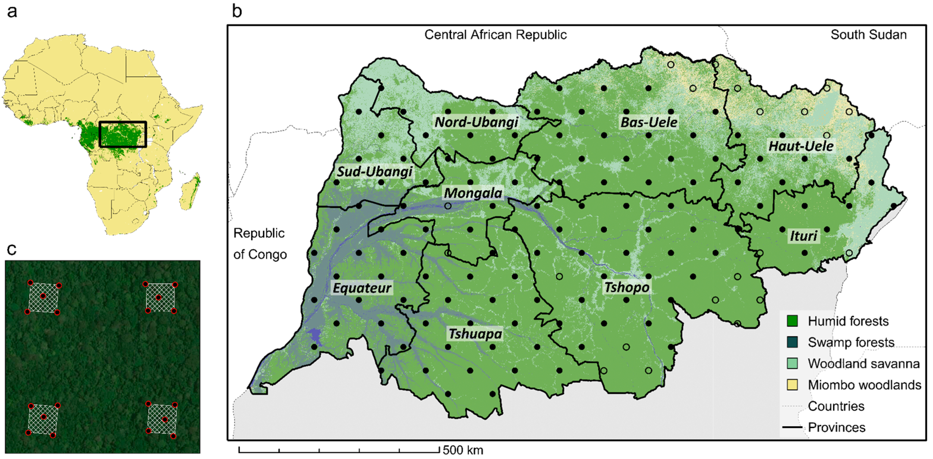
2.1. Study Area

The study area comprises the nine northern DRC provinces (out of 26 for the whole country), which span a total area of c. 900,000 km2, or about half the country. The mean altitude is 536 m (260–2436 m), the mean annual temperature is 24.6° (16.2–26.8°) and the mean annual precipitation is 1800 mm (878–2190 mm). The climate is characterized by two rainy seasons per year, usually starting around March (for two months) and October (for three months). The study area is dominated by forested lands and notably encompasses the vast majority of DRC’s humid forests (c. 624,000 km2, Figure 1b, [3]), corresponding to multi-strata, closed-canopy, large AGB, dense terra firme forests. The area also encompasses part of the peatland complex found in the Congo Basin which hosts a variety of swamp forest facies ranging from typical low-stature Raphia stands to high-stature dense forests on hydromorphic soils (c. 82,000 km2) [3]. Last, dryer, more open vegetated ecosystems (so-called Miombo woodlands, c. 29,000 km2) and woodland savannas (c. 160,000 km2) are found in the northern and northeastern parts of the study area.

2.2. Workflow of the Analysis

The methodological workflow of the analysis is shown in Figure 2. Our analysis combines two main data sources: (i) the maps produced by Xu et al. [18], particularly the national spaceborne biomass map that we briefly present in Section 2.3, and (ii) the DRC’s NFI, which we describe in Section 2.4.1 (sampling design) and Section 2.4.2 (field data protocol). We used the BIOMASS package (v. 2.1.5.9) published in 2017 by Réjou-Méchain et al. [20] to correct the NFI plots’ geographic coordinates and computed for each plot the AGB (and its uncertainty) from field inventory data (see Section 2.4.3). After extracting maps values at plot location (see Section 2.4.4), we compared map-derived biomass predictions (henceforth AGBmap) to field-derived biomass prediction (henceforth AGBfield) and population-level mean biomass estimates derived from the two data sources (see Section 2.5). All analyses were performed using the R statistical platform (v. 4.0.5).

2.3. DRC’s National Spaceborne Map

The national spaceborne map was published by Xu et al. [18] in 2017. The map covers the whole DRC at a 100 m spatial resolution and is representative of forest AGB circa the early 2010s. The reference set of observations is based on 432,000 ha of forest scanned with airborne LiDAR following a designed probability sampling methodology. LiDAR data were used to generate a raster of mean canopy height (MCH) at the mapping resolution (i.e., 100 m). Xu et al. [18] used a set of 92 1-hectare forest sample plots within the LiDAR flight paths to calibrate a power model describing the relationship between plot AGB, MCH and stand mean wood density (WD). This model was then used to predict AGB over the entire DRC based on country-wide maps of MCH and stand mean WD. To produce the country-wide map of MCH, Xu et al. [18] used a maximum entropy algorithm to extrapolate LiDAR-derived MCH based on Landsat 8 data, a digital elevation model derived from the Shuttle Radar Topography Mission (SRTM), L-band SAR data from the ALOS PALSAR sensor and a land cover classification (see [18] for details). The country-wide stand mean WD map was produced following the same extrapolation approach, but using 139 1-hectare forest sample plots as training data. The resulting maps of AGB predictions, prediction of uncertainty and the land cover classification are publicly available.

2.4. National Forest Inventory Data

2.4.1. Sampling Design

The DRC NFI was based on probabilistic sampling principles and used a systematic clustered sampling design. A triangular sampling grid was created and randomly positioned over the country. The grid was composed of isosceles triangles oriented along the N-S axis with bases measuring c. 110 km and equal sides c. 78 km. Each node of the grid was used as the origin of a sampling unit, which was composed of four square sample plots of 0.56 ha (i.e., 75 m × 75 m) spaced out by 250 m (Figure 1c) to limit spatial autocorrelation in measurements among plots. The sampling strategy brought a total of 321 sampling units spread over the country area, excluding Maï Ndombe, Kwilu and Kwango provinces, which were not targeted by the NFI, resulting in a sampling intensity of one sampling unit per c. 6.3 × 10³ km2. A total of 143 sampling units were located in the study area, 1 of which was located in the Congo River and 20 were not surveyed by the field teams due to local armed conflicts, notably in the North- and Southeastern edges of the study area. Among 122 remaining sampling units (representing 488 plots), 11 plots were not sampled due to conflicts with local populations and access difficulties (steep slopes). Therefore, the total number of plots for this study is 477.

2.4.2. Field Data

To perform the NFI field survey, ten field teams were simultaneously deployed by the Forest Inventory and Management Direction (“Direction des Inventaires et Aménagement Forestier”, DIAF) of the Ministry of Environment and Sustainable Development (“Ministère de l’Environnement et du Développement Durable”, MEDD). Each team was composed of two forest engineers from DIAF and a trained botanist from the University of Kisangani. Data collection over the study area (Figure 1b) corresponded to the first phase of the NFI and was performed between September 2017 and December 2018. For each sampling unit, the origins (S-W corner) of the four plots were provided to the field teams and located in the field using a handheld global positioning system (GPS) device (Garmin 64S). Plot limits were delimited using compasses and measurement tapes. To limit plot geolocation errors and facilitate spatial co-registration with remote sensing products, the geolocations of five locations per plot were recorded (i.e., the four corners and the plot center, Figure 1c) by averaging GPS measurements over a few seconds at each location.
Plot measurements followed a standard protocol. Each tree with a diameter at breast height (dbh) ≥ 20 cm was measured and identified, while trees in the 10–20 cm dbh range were sampled on two 0.06 ha subplots (i.e., 25 × 25 m) located on the S-W and N-E corners of the plot. Tree dbh was measured at 1.3 m height, or 30 cm above any buttresses or deformities. The height (h) of c. 50 trees distributed across the dbh range found in the plot were measured using a laser rangefinder device (TruPulse 360R). Herbarium specimens were collected on each tree for which the identification was uncertain and were stored at the Ecology and Forest Management Laboratory (LECAFOR) of Kisangani University. The total raw inventory dataset for the study area contains 46,963 tree dbh measurements and 13,365 h measurements. Of the 46,963 trees, 89.5% were identified at the species level, 6.6% at the genus level and 3.9% were left unidentified. Further database screening showed that some tree h measurements within 8 sampling units surveyed by the same field team were unrealistic. All h measurements from those sampling units were thus discarded, leaving a total of 12,359 h measurements in the dataset. Summary statistics on plot biophysical parameters are provided in Table S1.
Because of the systematic sampling design, some plots overlaid different land cover classes (e.g., humid forest, crops, etc.). For each plot, a sketch was drawn to represent the spatial distribution of land cover classes within the plot, following a detailed classification system containing 15 classes. For the purposes of this analysis, we simplified this classification system, aggregating NFI’s land cover classes into six aggregate classes that matched the land cover classification used by DRC in its Forest Reference Emission Level [3]: savannas, crops, natural regenerations on abandoned crops, dense humid forests on hydromorphic soil, terra firme dense humid forests and other forests. This simplified land cover classification was used for the establishment of tree height–diameter (h:dbh) allometric models (see Section 2.4.3).

2.4.3. Aboveground Biomass Prediction from Inventory Data

We used the BIOMASS package (v. 2.1.5.9) from Réjou-Méchain et al. [20] to predict sample plots’ aboveground biomass and their uncertainty.
The first step of the procedure consisted of attributing a wood density (WD) estimate (and its uncertainty) to each tree in the dataset. This was performed by the getWoodDensity function, which relies on WD measurements available in the Global Wood Density database (GWDdb [21,22]). For trees identified at species or genus levels, the mean WD of tropical African trees at the appropriate taxonomic level was used. The resulting set of mean WD is made available in [23]. When tree taxonomy was only available at the family level or trees were unidentified, the mean WD of trees found in the same sampling unit and land cover class was used. The getWoodDensity function provides the associated uncertainty for each mean WD estimate. This uncertainty is either based on the standard deviation of individual WD measurements used to compute the mean WD (when 10 measurements or more were used) or the standard deviation of individual WD measurements across the entire database (when less than 10 measurements were used).
Second, we built h:dbh allometric models to predict the height of trees that were not measured in the field. Given the high spatial variability in h:dbh relationships [24], we favored local h:dbh models (i.e., by land cover class within a sampling unit) over more generic, regional-scale models (i.e., by land cover class across the entire dataset). When ≥15 h measurements were available for a land cover class within a sampling unit (which represents 91.1% of the trees), a three-parameter Weibull distribution function [25] was fitted on those trees and used to predict the h of unmeasured trees within the same stratum. For the remaining 8.9% of trees in the dataset, h was predicted with regional land cover class specific h:dbh models fitted on the entire dataset (see Figure S1). h prediction uncertainty for each tree in the dataset was computed as the residual standard error of the corresponding h:dbh model.
Third, to account for the partial sampling of trees in the 10–20 cm dbh range, we followed the procedure described in [26]. This procedure is embedded in the Monte Carlo computation scheme described in the subsequent paragraph and allows simulating, for each plot, the missing inventory data (i.e., tree diameters and identifications) for trees in the 10–20 cm dbh range that were not sampled on the entire plot (i.e., so-called specific functions 1 and 2 in [26]). In practice, this procedure (i) expands the count of trees in the 10–20 cm dbh class from the observed count c in the spatial fraction p of the plot that was actually surveyed to the entire plot area by randomly generating a value from a negative binomial distribution X~NegBin(c, p), (ii) assigns species labels to simulated trees at the pro-rata of species abundance observed in the p fraction of the plot and (iii) assigns a continuous diameter to each simulated tree by inverse transform sampling from a two-parameter Weibull distribution function, with a scale parameter λ = 8.593 and a shape parameter k = 0.737.
Fourth, we used a Monte Carlo procedure to compute the AGB of each tree (and its uncertainty) with the pantropical AGB allometric model (Equation (4) in [27]). The procedure propagates uncertainties arising from the simulation of missing inventory data, WD, h, and the allometric model to tree AGB predictions (see [26] for details). The output of the procedure is a vector of 1000 AGB replicates per tree. For a given sample plot, the output matrix can thus be summed by Monte Carlo iterations to obtain a vector of 1000 replicates of plot AGB (i.e., A G B i t e r , with iter in (1–1000)), which incorporates the different sources of uncertainty. Each A G B i t e r replicate represents a realization of plot AGB for trees with dbh ≥ 10 cm over the plot area, i.e., 75 × 75 m or 0.56 ha, which we assumed to be error-free. A G B i t e r replicates were thus divided by the plot area to provide an AGB prediction per hectare and allow for comparison with biomass density values of the national spaceborne AGB map.
Last, to account for trees in the range of 1–10 cm dbh, we used the model proposed by Xu et al. [18]:
A G B 1 cm = 1.872 A G B i t e r 0.906
Following Xu et al. [18], we assumed that scaling up A G B i t e r to A G B 1 cm propagated a negligible uncertainty. The mean of the A G B 1 cm vector was then used as our field prediction of plot AGB (i.e., A G B f i e l d ).

2.4.4. Linking Field Plots to the National Spaceborne Biomass and Land Cover Maps

An important issue when evaluating a map is to accurately position reference data. Under forest canopy, the error on a GPS measurement acquired with a precise receiver commonly exceeds 20 m, and can be as high as 200 m [13,28]. Therefore, reducing plot geolocation errors requires using GPS measurements at multiple locations of the plot, so that random GPS errors average out [13]. For each plot, we leveraged all (usually five) GPS measurements to determine the most probable plot geolocation using the correctCoordGPS function of the BIOMASS R package. The correctCoordGPS function performs a procrust (translation, rotation) on the set of GPS coordinates while preserving the plot size (75 m × 75 m) and a squared shape. For some plots, a few GPS measurements were either missing or unrealistic (e.g., located ≥100 km from the plot center). To avoid introducing errors in the assessment of the national spaceborne AGB map associated with spatial mismatches between the map and the reference data, we discarded all plots with less than three GPS measurements (n = 7). For the remaining 470 plots, we extracted (i) the area-weighed means of AGB values in the national spaceborne AGB map (hereafter A G B m a p , Equation (2)) and (ii) the modal class of the land cover map used in the construction of the national spaceborne model, for pixels that intersected the plots.
A G B m a p = 1 X ( A G B x × a x ) 1 X ( a x )
where A G B x is the map AGB prediction for pixel x, a x is the area of pixel x intersected by the plot and X is the total number of intersected map pixels.

2.5. Statistical Analyses

2.5.1. Assessment of Map Predictive Power at Plot Locations

We compared the national spaceborne biomass map predictions at plot locations (i.e., A G B m a p ) to field-based predictions (i.e., A G B f i e l d ) using the squared correlation between the two datasets (denoted R2, Equation (3)), a metric of average error (denoted B, Equation (4)), the root mean square error (RMSE, Equation (5)) and the coefficient of variation (CV, Equation (6)).
R 2 = C o r ( A G B m a p ,   A G B f i e l d ) 2  
B = ( A G B m a p ^ A G B f i e l d ^ ) A G B f i e l d ^
R M S E = 1 n 1 n ( A G B m a p ,   i A G B f i e l d ,   i ) 2
C V = R M S E A G B f i e l d ^ × 100
where n is the number of sample plots, A G B m a p ,   i and A G B f i e l d ,   i are the biomass of plot i extracted from the map and derived from field data, respectively, and A G B m a p ^ and A G B f i e l d ^ are their mean across the n plots.
While A G B f i e l d data are assumed to be of greater quality (that is, of greater accuracy) [29] than A G B m a p , both sets of predictions are subject to a non-negligible uncertainty. In Section 2.4.3, we described the Monte Carlo procedure used to generate 1000 AGB replicates by plot, incorporating and allowing the quantification of the uncertainty on A G B f i e l d . The uncertainty on map AGB predictions have also been made available at the pixel level in Xu et al. [18], and can be aggregated among pixels intersected by each plot (SEplot) using standard error propagation rules. To account for the imperfect nature of AGB predictions when evaluating the national spaceborne map, statistics of map predictive power (i.e., R2, B, RMSE and CV) were computed by comparing each of the 1000 plot AGB replicates (i.e., A G B 1 cm ) to a realization of A G B m a p , defined as the sum of A G B m a p to an error randomly drawn from the distribution N(0, SEplot,i). This led to a vector of length 1000 for each performance metric, from which we report the mean and its 95% confidence interval.
The temporal mismatch between the biomass map (which is representative of the early 2010s) and NFI data (which were acquired in 2017–2018) may also introduce uncertainty in the assessment of map predictions. For example, if a forested land was converted to a crop in the year 2015, the map would display a large biomass for that land while the biomass prediction from NFI data would be small, hence resulting in a large prediction error for the map. This prediction error would not reflect the predictive performance of the mapping model but would be attributable, in this example, to the 2015 land cover change. To further investigate the influence of this temporal mismatch, we used GLAD (Global Land Analysis & Discovery) vegetation loss data [30] to remove all plots where one (or more) vegetation loss was detected in the 2010–2017 period. Map validation statistics were then computed using both the full set of 470 plots and the subset of undisturbed plots (n = 411).

2.5.2. Design-Based Inference from the Field Sample Plots and Error Propagation

AGB per unit area for the whole area of study and for the subpopulations of interest was estimated using field plots data. The field plots were treated as a systematic cluster sample of size n = 122. The 122 elements in the sample represent all clusters in which at least one plot was accessible by the field crews and whose tree variables could be measured. The average AGB per unit area was estimated using ratio estimators [31,32], which are widely used for estimating population parameters in large-area forest surveys [33,34,35,36,37]. The ratio estimators were chosen because of the ability to accommodate cluster plots with partial nonresponse [38] and because they can be used efficiently for providing estimates for targeted subpopulations (also known as domains), such as forest types and administrative boundaries [37,39,40]. For estimation purposes, we assume that the set of nonresponse plots is missing at random, and they are not systematically different from the responding ones [41]. The population AGB per unit area is estimated using the following ratio estimator (also known as ratio-to-size estimator [32,40,42]):
μ ^ R A T I O = j = 1 n A G B c l u s t e r ,   j j = 1 n a   j
V a r ^ ( μ ^ R A T I O ) = n ( n 1 ) j = 1 n ( A G B c l u s t e r ,   j a   j μ ^ R A T I O ) 2 j = 1 n ( a   j ) 2
where n is the total sample size (n = 122), A G B c l u s t e r ,   j is the aboveground biomass estimated from the inventory data in the jth cluster and a   j is the area of the jth cluster which was accessible by the field crew. Averages by land use class and provinces are also estimated using the following domain ratio estimators:
R ^ d = j = 1 n A G B c l u s t e r ,   j , d j = 1 n a   j , d
V a r ^ ( R ^ d ) = n ( n 1 ) j = 1 n ( A G B c l u s t e r ,   j , d a   , d j μ ^ R A T I O ) 2 j = 1 n ( a   j , d ) 2
where A G B c l u s t e r ,   j , d is the aboveground biomass estimated from the inventory data in domain d and in the jth cluster and a   j , d is the area of the jth cluster falling into domain d that was accessible by the field crew. Despite the fact that V a r ^ ( μ ^ R A T I O ) and V a r ^ ( R ^ d ) from Equations (8) and (10) may be biased when applied to systematic sampling, they are likely to overestimate the variance [31], offering an acceptable conservative approach to the sample estimates. It is worthwhile to notice that the variance estimators (Equations (8) and (10)) account for the fact that both the aboveground biomass and the area measured are random variables.
The uncertainties arising from the missing inventory data, WD, h and the allometric model obtained through the Monte Carlo simulation procedure described in Section 2.4.3 were propagated to the large-area estimates of mean AGB following the methodology provided by [41] (see also [43]). For each k t h Monte Carlo replication, the mean AGB, μ ^ k and variance of the mean V a r ^ ( μ ^ k ) for the overall study area and for each domain were estimated using the ratio estimators (Equations (7)–(10)) described above. The mean and variance over replications were estimated by:
μ ^ = 1 n r e p k = 1 n r e p μ ^ k
V a r ^ ( μ ^ ) = ( 1 + 1 / n r e p ) W 1 + W 2
where n r e p is the number of replications, W 1 = ( n r e p 1 ) 1 k = 1 n r e p ( μ ^ k μ ^ ) is the among-replication variance and W 2 = ( n r e p 1 ) 1 k = 1 n r e p V a r ^ ( μ ^ k ) is the mean variance within replications.

2.5.3. Model-Based Inference from the Biomass Map

For the calculation of mean biomass over large regions from the biomass map, we used the model-based estimator (MB) given in Equation (13), which simply consists of averaging map predictions over the region of pixels.
μ ^ M B = 1 N × i = 1 N A G B m a p ,   i
where i indexes the pixels and N is the total number of pixels within the region. We did not compute the variance of the MB estimate, which would require additional information on the biomass map, such as the spatial autocorrelation among the residuals, which were not available.

3. Results

3.1. Predictions of Plot-to-Plot Biomass Variation

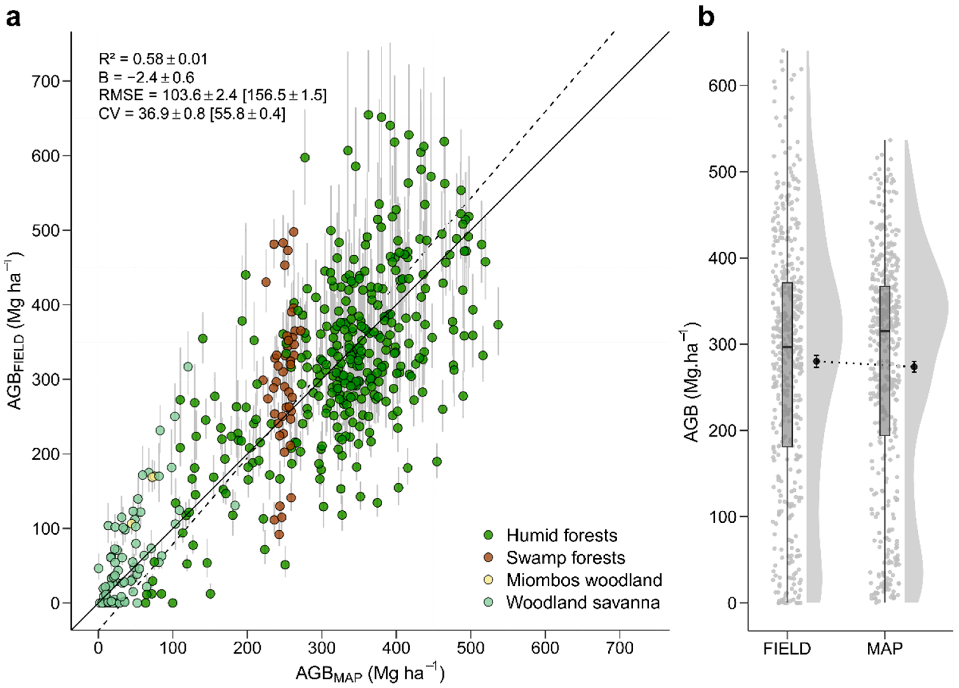
3.1.1. Relationship between AGBMAP and AGBFIELD across All Plots

Using the full set of 470 sample plots, we found that the map predicted 58% of AGBFIELD variation (Figure 3a) with an average prediction error (RMSE) of 103.6 Mg ha−1 or 36.9% (CV). The relationship between AGBFIELD and AGBMAP was slightly biased (slope of Major Axis regression: 1.16, 95% CI: 1.08–1.25), leading to a small underestimation of the biomass across plots (B = −2.4%, Figure 3b). Removing plots where a loss of vegetation cover was detected between 2010 and the establishment of NFI sample plots (hereafter “disturbed” plots, n = 59) did not lead to noticeable changes in the results (Figure S2).

3.1.2. Mapping Error by Classes of AGBFIELD

Breaking down the assessment of map prediction error by AGBFIELD classes of 50 Mg ha−1 width, we found that map predictions were nearly unbiased on the early range of biomass (0–150 Mg ha−1, Figure 4a), which mostly comprised non-forest and open-canopy forest areas (Figure 3a). Beyond 150 Mg ha−1, map prediction error showed a non-linear pattern of bias. Across plots of intermediate biomass (c. 150–300 Mg ha−1), the map showed a moderate positive median error (c. 24.5–47.0 Mg ha−1, Figure 4a). From 300 Mg ha−1 onward, map prediction error decreased as AGBFIELD increased, becoming negative around c. 350 Mg ha−1 and further decreasing up to the largest values of AGBFIELD, which were largely underestimated (median error: −234.6 Mg ha−1, n = 10). Removing disturbed plots unveiled a simpler bias pattern beyond 150 Mg ha−1 consisting of a single linear decreasing trend (Figure S3a). This bias pattern suggests a loss of map predictive power on the second half of the AGBFIELD range. Using piecewise regression, we found a significant breakpoint in the AGBMAPAGBFIELD relationship at 286 Mg ha−1 (Davies’ test p < 0.0001, Figure 4b), after which the linear correlation between AGBMAP and AGBFIELD was weak (R2 = 0.1). The location of the breakpoint did not change when excluding disturbed plots (Figure S3b).

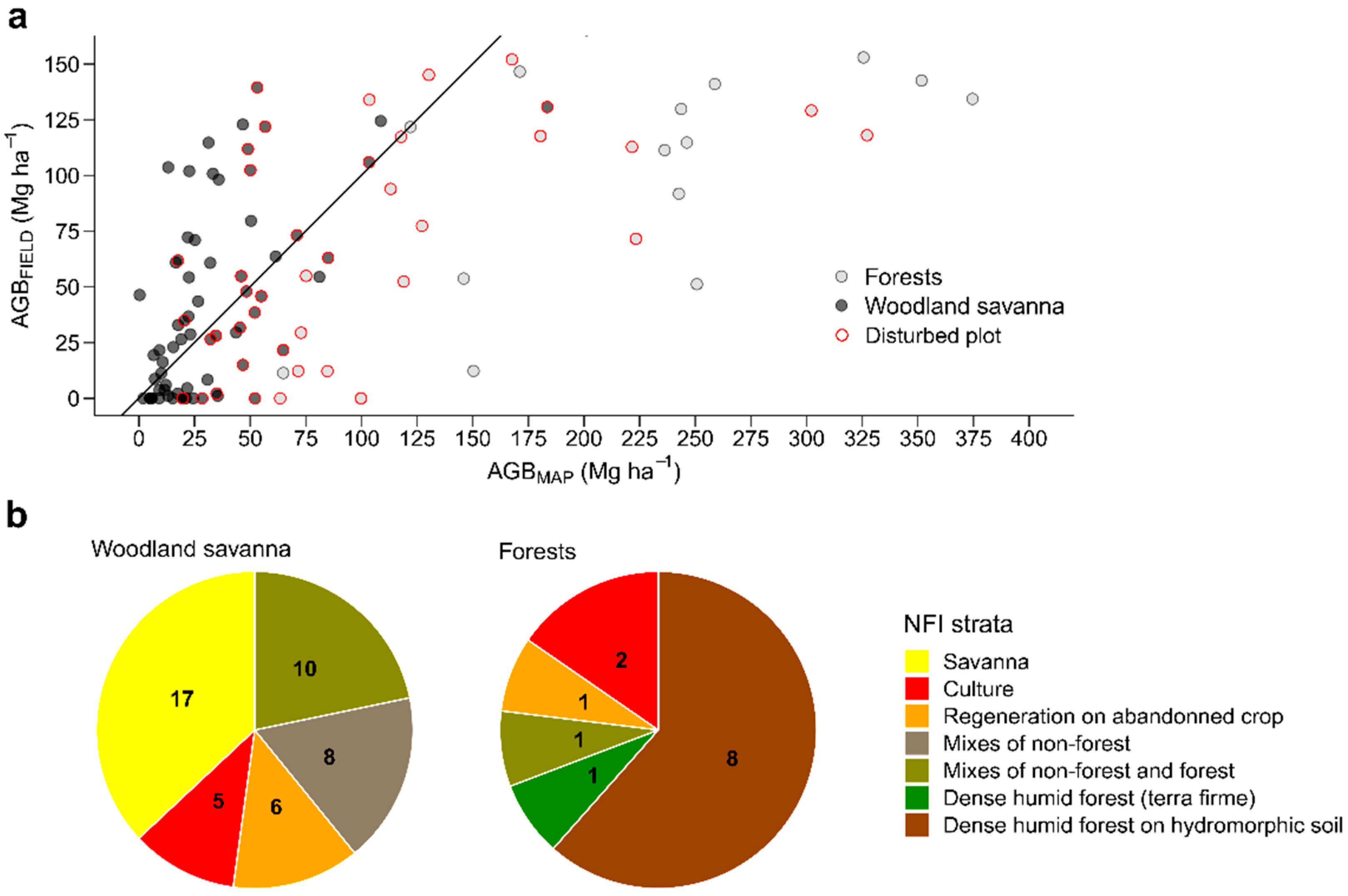
3.1.3. Relationship between AGBMAP and AGBFIELD per Landcover Classes

We split the set of plots by landcover classes and assessed map predictions within classes, excluding the Miombos woodland class which only contained three plots.
Unsurprisingly, the map explained a greater share of AGBFIELD variation in the small-biomass class of woodland savanna (R2 = 0.41) than in larger-biomass forest classes (Table 1). In the latter classes, the map captured 33% of AGBFIELD variation within humid forests, and did not discriminate any AGB variation within swamp forests (as seen in Figure 3a). This pattern of map predictive error among landcover classes is consistent with the notion of signal saturation for larger AGBFIELD values (≥c. 290 Mg ha−1) and was strengthened when removing disturbed plots, with a higher predictive power on woodland savanna (R2 = 0.58) and a lower predictive power on humid forests (R2 = 0.20, Table S2).
It is noteworthy that map predictions on the set of NFI plots were virtually unbiased in humid forests (B < 1%) but underestimated the average biomass of swamp forest plots by 17.5% and that of woodland savanna plots by 33.2%. Removing disturbed plots accentuated the negative bias on the woodland savanna class (B = −45.0%, Table S2). Since map predictions were nearly unbiased on the early biomass range (0–150 Mg ha−1), the large underestimation of biomass in the woodland savanna class shows that this negative bias was in fact balanced by a positive bias on plots classified as forests (either swamp or humid) in this biomass range (Figure 5a). Landcover classification based on field observations made during the NFI showed that undisturbed plots classified as woodland savanna by the landcover map in fact corresponded to a variety of non-forest classes. These classes are commonly found in the agro-mosaic landscape of Central Africa, including savanna (37.0%), crops (10.9%), natural regeneration on abandoned crop (13.0%) and mixes of non-forest (17.4%) or non-forest and forest (21.7%) classes (Figure 5b). Concerning undisturbed plots classified as forest by the landcover map, most plots (i.e., 69.2%) indeed corresponded to forest classes in the NFI classification (notably forests on hydromorphic soil) but with much smaller biomass value than that predicted by the map, while the remaining plots were attributed to non-forest classes (Figure 5b), reflecting classification errors in the landcover map.

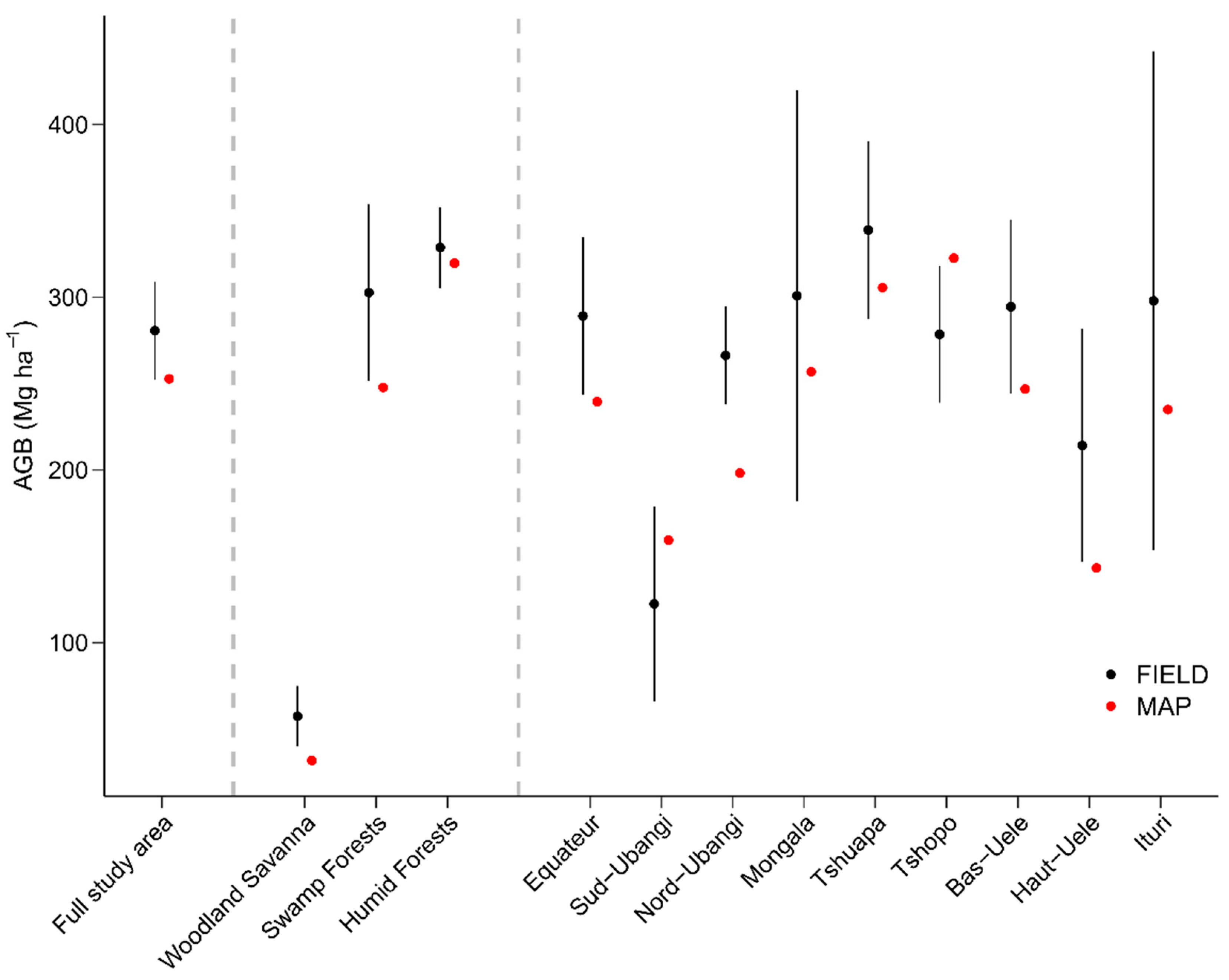
3.1.4. Predictions of Mean Biomass at Population Level

We used the field sample plots to compute mean biomass estimates at different scales (i.e., the full study area, the land cover classes, the provinces) and compared these estimates to the ones obtained from the biomass map.
At the scale of the study area, the mean biomass estimate derived from field sample plots was 280.6 Mg ha−1, and its 95% CI (252.2–309.0 Mg ha−1) included the estimate derived from the map (i.e., 252.7 Mg ha−1, Figure 6).
Among land cover classes, both data sources led to similar mean biomass estimates for the humid forests class (i.e., 328.8 and 319.7 Mg ha−1 for field sample plots and the map, respectively), but using field plots led to larger mean biomass estimates for woodland savanna (i.e., 57.3 Mg ha−1, 95% CI: 39.8–74.9 Mg ha−1) and swamp forests classes (i.e., 302.7 Mg ha−1, 95% CI: 251.6–353.7 Mg ha−1) than using the map (i.e., 31.8 and 247.8 Mg ha−1, respectively).
Among provinces, 95% CIs around mean biomass estimates derived from field sample plots were large owing to the relatively small number of plots by provinces (ranging from 28 to 97 Mg ha−1, see Table S3 for details) and included mean biomass estimates from the map in six out of the nine provinces. At the province scale, the general trend observed is that using field sample plots led to larger mean biomass estimates as compared to estimates from the map. This observation is consistent with the results obtained with mean biomass estimates per land cover classes. In contrast, the mean biomass estimates for the Sud-Ubangui and Tshopo provinces were larger with the map than with field plots, indicating that the deviation between map and field mean biomass estimates differed in those provinces from the regional trend. In the Tshopo province, for instance, where the humid forest class covered 92.3% of the land, the mean biomass estimate for that class was larger with the map (341.3 Mg ha−1) than with field sample plots (292.6 Mg ha−1, Figure S4).

4. Discussion

Validation of RS-derived maps is both essential to compare and improve mapping methodologies and to build confidence in mapping products and support their adoption by end-users [44]. Here, we performed an assessment of the national spaceborne AGB map of DRC using NFI data regularly distributed over the northern part of the country, which hosts the majority of the Congo basin dense forests, an ecosystem for which AGB mapping is notoriously challenging. Our results show that the map predicts about 60% of plot-to-plot variation in field-derived AGB, but that its predictive performance is not homogeneous along the AGB gradient. Here, we discuss our findings and their implications in using map-derived AGB in the context of REDD+ and forest management.

4.1. The Overall Relationship between RS- and Field-Derived AGB Predictions Is Coherent

An important challenge when mapping forest AGB over a geographic extent as broad as the one covered by the DRC country (2.3 Million km²) is to build a prediction model that is sufficiently general, i.e., that allows producing reliable AGB predictions in areas that are far apart from model training data, which necessarily represent a tiny fraction of the study area. To cope with the lack of field-derived reference data available to train RS models and the potential bias in their spatial distribution, which limits their representativity of the study area [45], it is increasingly recognized that a two-stage calibration strategy leveraging aerial LiDAR data is adequate [10,13]. In practice, the limited set of field inventory data is used to train aerial LiDAR data, and LiDAR-derived predictions are then used to calibrate the wall-to-wall RS model, which largely expands the size of the RS model training dataset. This strategy, which was used by Xu et al. [18], has been successfully employed on relatively small geographic areas (i.e., from a few hundreds to thousands km2), but implementations at the country scale and independent assessments of the resulting maps remain seldom (but see [46] for an implementation over Peru). Despite the vast geographic extent of DRC and the availability of only 92 1-hectare plots clustered in a few sampling sites to calibrate the LiDAR-model, our results show that the mean deviation (or bias) of map AGB predictions at NFI plot locations is smaller than 3%. Furthermore, the national spaceborne map explained about 60% of plot-to-plot variation in AGB across all plots, which is well within the range of results reported by local case studies using spatial cross-validation [14,47] and confirms the scalability of the two-stage calibration strategy.

4.2. The RS Signal Saturates on Dense Forests—But at Relatively Large AGB Levels

While map validation statistics over the entire AGB gradient sampled by NFI plots were satisfying, we nonetheless observed a saturation phenomenon in the relationship between map- and field-derived AGB predictions around c. 290 Mg ha−1, above which the map’s ability to predict plot-to-plot variation was weak (R2 = 0.1). The saturation of multispectral imagers on large-biomass forest has been widely reported and the AGB threshold at which the loss of sensitivity occurs varies among sensors and forest types. Interestingly, the saturation threshold found in the present study is higher than that usually reported for Landsat data (100–200 Mg ha−1) [48] and even higher spatial resolution imagers (e.g., 250 Mg ha−1 for Worldview-3 [14]). We suggest that two main reasons explain this difference. First, Xu et al. (2017) used both Landsat and L-band ALOS PALSAR imagery to extrapolate LiDAR-derived predictions. The positive relationship between L-band backscatter and AGB has been widely used in AGB mapping studies, which usually report an attenuation of the signal around c. 150 Mg ha−1. While this attenuation is interpreted as a complete loss of sensitivity (saturation), it has been shown that the relationship between L-band backscatter and forest AGB changes on dense forest canopies but could remain informative far beyond 150 Mg ha−1 [49]. It is thus possible that by using the MAXENT algorithm, which accommodates for non-linear relationships between model’s covariates and the dependent variable, the inclusion of L-band radar in the mapping model allowed widening its range of sensitivity. Second, Xu et al. (2017) mapping methodology consisted of separately mapping forest canopy height and stand wood density prior to fusing the two maps into an AGB map. In contrast with the more common methodology which consists of directly relating spaceborne data to forest AGB, the indirect approach used in Xu et al. [18] may better model variation in forest structure—through canopy height—and in fine capture more spatial variability in AGB. Indeed, variation in stand wood density among field sample plots may have “noise” in field-derived AGB predictions that cannot be predicted by the mapping model, as current wall-to-wall spaceborne sensors have shown some sensitivity to variation in forest structure, such as forest canopy height [50], while mapping wood density remain challenging [51].

4.3. The Map Shows Contrasted Performances within Landcover Classes

We used a simple landcover classification composed of two classes of forests (humid and swamp) and a single non-forest class (woodland savannas) to disaggregate the map predictive performance by landcover classes. Given the non-homogenous performance of the map along the AGB gradient (i.e., saturation) and the structuration of landcover classes along this gradient, we naturally observed contrasted map performances per landcover classes.
The mean biomass for forest classes (i.e., 303 and 329 Mg ha−1 for swamp and humid forests, Table S3) were above the saturation threshold of the spaceborne mapping model, leading to a weak correlation between map predictions and field-derived AGB predictions, with R2 values of 0.20 and 0.02 on humid and swamp forests (after excluding disturbed plots, Table S2), respectively. While map predictions were unbiased on the humid forest class (B < 1%), which cover most of our study area, we observed a systematic under-estimation of swamp forests AGB (c. −17.5%, Table S2). We suspect that the relatively poorer performance of the map on swamp over humid forests, both in terms of ability to capture the AGB gradient and the mean of the distribution, is related to the lack of field sample plots from this forest class in the training set of the national spaceborne mapping model (i.e., a single swamp forest plot, information from the authors of [18]). Since swamp forests are clearly discernable from terra firme forest in optical very-high-resolution spaceborne data, and given the influence of humidity on the radar signal, it is indeed likely that relationships between the model’s covariates and forest AGB differs among swamp and humid forests.
As expected, the map showed a much higher predictive power on plot-to-plot AGB variation in woodland savannas (R2 = 0.58, Table S2), where the mean plot AGB (i.e., 57.3 Mg ha−1, Table S3) was much smaller than the saturation threshold of the mapping model. While a common bias pattern in biomass mapping models is to over-estimate small AGB values and to under-estimate large AGB values [14,15], map predictions were—at first glance—nearly unbiased below the model saturation threshold. However, decomposing map predictive performance by landcover classes revealed a more complex pattern of error among small AGB plots, with a large under-estimation of AGB on woodland savanna plots (B = −45%) and an over-estimation of AGB on forest plots in the range 0–150 Mg ha−1 (Figure 5a). A possible reason for the underestimation of vegetation AGB in woodland savannas could be, again, an improper calibration of the LiDAR model due to a lack of field data, since only five plots located in savannas were available for model training.

4.4. Implications for DRC’s Carbon Emissions Reporting and Outlooks

The recent availability of a NFI in DRC gives to the country, for the first time, the opportunity to estimate mean carbon stocks of landcover classes in a design-based inferential framework, warranting the unbiasedness of the estimates [13].
Using a ratio estimator, we obtained an estimate of mean AGB for the dominant humid forest class that was very close to the estimate derived from the national spaceborne map, but mean AGB estimates for the two other landcover classes (i.e., swamp forest and woodland savanna) differed markedly between the two data sources (Figure 6). We thus do not recommend the use of the national spaceborne map in a model-based inferential framework to compute landcover classes mean carbon stocks, and in fine national emission factors, for REDD+ MVR (Measurement, Verification and Reporting) under UNFCCC (United Nations Framework Convention on Climate Change). This is not to say that the current national spaceborne map or the tremendous investment made to acquire aerial LiDAR data over the country cannot be valued in REDD+ framework.
The logical next step to this study would be to assess the usefulness of the current national spaceborne map to reduce the uncertainty on landcover class mean carbon stocks when combined with (rather than separately from) NFI plots. For instance, the map could be leveraged to increase the precision of the AGB estimates in the context of design-based inference through model-assisted estimation [13], which still relies on the probabilistic nature of the NFI plot design and warrants the unbiasedness of resulting estimates, despite potential biases in the map. Such an approach has proven to reduce the standard error on mean carbon stocks by more than twofold on Miombo woodlands of Tanzania [52], for example. Auxiliary data coming from the national spaceborne map can also be used to address the non-response in ground data collection, in combination with special estimation techniques such as weighting or imputation [41,53].
The current acquisition of GEDI data [54] and the availability of NFI data also open avenues to improve the DRC national spaceborne carbon map. GEDI data, for instance, could be integrated in the AGB mapping chain in several ways, either in addition to aerial LiDAR data in the training dataset of the forest canopy height mapping model, or as an independent validation dataset. In the latter case, the independent set of GEDI canopy height measurements could be used to select the covariates of the mapping model so as to maximize its transferability in space [55]. Similarly, the large size of the NFI dataset, its regular distribution over DRC and its independence from the data used to build the national spaceborne AGB map make NFI data an ideal validation dataset both to refine the functional forms of the models used to build the AGB map (i.e., canopy height and wood density mapping models) and to assess the uncertainty of the final AGB product. Last, we also suggest that the landcover map used in the AGB mapping chain should match the official landcover stratification used by DRC in its international greenhouse gas reporting, which would facilitate the adoption of the AGB map by the country.

5. Conclusions

We performed an assessment of the DRC’s national spaceborne AGB map using field inventory data from the country’s NFI. Our results show a coherent and nearly unbiased relationship between map prediction and NFI’s sample plot AGB across all plots, with a relatively high saturation threshold (c. 290 Mg ha−1) considering known limits of spaceborne wall-to-wall data (i.e., signal saturation). Decomposing this relationship by landcover classes, however, we found that the map explained more AGB variability in the small AGB class (woodland savannas) than in large AGB classes (humid and swamp forests). In contrast, map predictions tended to over-estimate AGB in the small AGB class while being closer to mean biomass predictions in large AGB classes. We attribute this error pattern to the uneven distribution of field sample plots across landcover classes when calibrating the mapping model and to the relatively weak relations existing between current wall-to-wall spaceborne data and AGB in large AGB tropical forests.

Supplementary Materials

The following supporting information can be downloaded at: https://www.mdpi.com/article/10.3390/rs14164126/s1, Figure S1: Regional h:d models per landcover stratum derived from NFI data (DHF TF: dense humid forest terra firme; DHF HS: dense humid forest on hydromorphic soil; Sav.: savanna; Cult.: culture; Regen. cult.; regeneration on abandoned crop; Other: other landcover type). Parameters of the three-parameter Weibull model ( h = a × ( 1 e x p ( d c b ) ) , with h and d the tree height and the trunk diameter, respectively) are provided between brackets; Figure S2: Scatterplot of sample plots aboveground biomass derived from inventory data (AGBFIELD) and vs the biomass map (AGBMAP). AGBFIELD estimates are bounded by their 95% confidence interval (grey segments). The dash line represents the fit of a major axis regression. For information, disturbed plots are highlighted by red crossed circles, but these plots were not used when computing map performance statistics and fitting the major axis regression model; Figure S3: a., Breakdown of mapping error by classes of aboveground biomass derived from inventory data (AGBFIELD). b., Breakpoint in the relationship between sample plots aboveground biomass derived from the biomass map (AGBMAP) and AGBFIELD. The red line represents the fit of a piecewise regression. The dashed vertical line highlights the location of the breakpoint. For information, disturbed plots in a and b are highlighted by red crossed circles, but are not used when generating boxes (a) or fitting the pricewise regression (b); Figure S4: Provincial distributions of aboveground biomass (AGB) in field sample plots (red) and in the map (dark grey) for the Humid forests class. Distribution means are represented with thick circles (bounded by ± one s.e.); Table S1: Biophysical parameters of forest samples plots from the National Forest Inventory. N stands for the number of trees, G for plot’s basal area (in m2 ha−1), Dg for the quadratic mean tree diameter (in cm), WDp for the basal area-weighted wood density (in g cm−3), H98 for the 98th quantile of tree predicted height (in m) and AGB for the aboveground biomass (in Mg ha-1); Table S2: Relationships between field- and map-derived plots aboveground biomass by land cover class. Disturbed plots were removed from the analysis. N, R2, B, RMSE and CV stand for the number of plots, the squared correlation, the average error, the root mean squared error and the coefficient of variation, respectively; Table S3: Mean biomass estimation (in Mg ha−1) by stratum using field sample plots (including “disturbed” plots) and the biomass map. N and CI stand for the number of plots and the confidence interval, respectively.

Author Contributions

A.L., P.P. and J.-P.K.L. conceived the study and led the writing of the paper. A.L., P.P. and L.B. analyzed the data. L.B., L.X. and S.S. commented on the analyses and provided critical inputs for the writing of the paper. All authors have read and agreed to the published version of the manuscript.

Funding

P.P. was supported by a postdoctoral grant from the Centre national d’études spatiales (CNES) and from the 3DForMod project, funded in the framework of the ERA-NET FACCE ERA-GAS (ANR-17-EGAS-0002-01), which has received funding from the European Union’s Horizon 2020 research and innovation program under grant agreement no. 696356.

Acknowledgments

We are deeply grateful to DRC’s Ministère de l’Environnement et du Développement Durable (MEDD) for granting us access to the NFI’s data. In particular, we would like to stress out the continuous and effective support of Benjamin Toirambe Bamoninga, General Secretariat of MEDD, for the NFI data use and access. We would also like to dedicate this article to André Kondjo Shoko, who passed away recently, as he played a critical and central role for the achievement of the first ever DRC national forest inventory. In his position as Head of the Forest Inventory Division within the Direction des Inventaires et Aménagement Forestier (DIAF) of the MEDD, he greatly contributed to all phases of the preparation and the realization of the fieldwork with exemplary rigor and self-denial. Might the present article be a recognition of his immense and long-term engagement for improving the scientific knowledge and the management of DRC forests. Finally, we would like to thank the four anonymous referees for their comprehensive reviews which substantially improved the first version of the manuscript.

Conflicts of Interest

The authors declare no conflict of interest.

References

  1. Mitchard, E.T.A. The Tropical Forest Carbon Cycle and Climate Change. Nature 2018, 559, 527–534. [Google Scholar] [CrossRef] [PubMed]
  2. Tyukavina, A.; Hansen, M.C.; Potapov, P.; Parker, D.; Okpa, C.; Stehman, S.V.; Kommareddy, I.; Turubanova, S. Congo Basin Forest Loss Dominated by Increasing Smallholder Clearing. Sci. Adv. 2018, 4, eaat2993. [Google Scholar] [CrossRef] [PubMed] [Green Version]
  3. Ministère de l’Environnement et Développement Durable. Niveau d’Emissions de Référence Des Forêts; Ministère de l’Environnement et Développement Durable: Kinshasa, Democratic Republic of the Congo, 2018.
  4. United Nations. World Population Prospects: The 2017 Revision, Key Findings and Advance Tables; UN: New York, NY, USA, 2017. [Google Scholar]
  5. Kengoum Djiegni, F.; Pham, T.T.; Sonwa, D.J. Dix Ans de REDD+ Dans Un Contexte Politique Changeant En République Démocratique Du Congo; CIFOR Infobrief: Bogor, Indonesia, 2020. [Google Scholar]
  6. Sandker, M.; Crete, P.; Lee, D.; Sanz-Sanchez, M. Considérations Techniques Relatives à l’établissement de Niveaux d’émissions de Référence Pour Les Forêts et/Ou Niveaux de Référence Pour Les Forêts Dans Le Contexte de La REDD+ Au Titre de La CCNUCC; FAO: Rome, Italy, 2016; ISBN 978-92-5-208841-7. [Google Scholar]
  7. Nesha, M.K.; Herold, M.; Sy, V.D.; Duchelle, A.E.; Martius, C.; Branthomme, A.; Garzuglia, M.; Jonsson, O.; Pekkarinen, A. An Assessment of Data Sources, Data Quality and Changes in National Forest Monitoring Capacities in the Global Forest Resources Assessment 2005–2020. Environ. Res. Lett. 2021, 16, 054029. [Google Scholar] [CrossRef]
  8. Herold, M.; Carter, S.; Avitabile, V.; Espejo, A.B.; Jonckheere, I.; Lucas, R.; McRoberts, R.E.; Næsset, E.; Nightingale, J.; Petersen, R.; et al. The Role and Need for Space-Based Forest Biomass-Related Measurements in Environmental Management and Policy. Surv. Geophys. 2019, 40, 757–778. [Google Scholar] [CrossRef] [Green Version]
  9. McRoberts, R.E.; Tomppo, E.O.; Næsset, E. Advances and Emerging Issues in National Forest Inventories. Scand. J. For. Res. 2010, 25, 368–381. [Google Scholar] [CrossRef]
  10. Réjou-Méchain, M.; Barbier, N.; Couteron, P.; Ploton, P.; Vincent, G.; Herold, M.; Mermoz, S.; Saatchi, S.; Chave, J.; de Boissieu, F. Upscaling Forest Biomass from Field to Satellite Measurements: Sources of Errors and Ways to Reduce Them. Surv. Geophys. 2019, 40, 881–911. [Google Scholar] [CrossRef]
  11. Rejou-Mechain, M.; Muller-Landau, H.C.; Detto, M.; Thomas, S.C.; Le Toan, T.; Saatchi, S.S.; Barreto-Silva, J.S.; Bourg, N.A.; Bunyavejchewin, S.; Butt, N.; et al. Local Spatial Structure of Forest Biomass and Its Consequences for Remote Sensing of Carbon Stocks. Biogeosciences 2014, 11, 6827–6840. [Google Scholar] [CrossRef] [Green Version]
  12. Knapp, N.; Huth, A.; Fischer, R. Tree Crowns Cause Border Effects in Area-Based Biomass Estimations from Remote Sensing. Remote Sens. 2021, 13, 1592. [Google Scholar] [CrossRef]
  13. Duncanson, L.; Armston, J.; Disney, M.; Avitabile, V.; Barbier, N.; Calders, K.; Carter, S.; Chave, J.; Herold, M.; Macbean, N. Aboveground Woody Biomass Product Validation Good Practices Protocol. Version 1.0; CEOS Working Group on Calibration and Validation; Lanf Product Validation, 2021. Available online: https://lpvs.gsfc.nasa.gov/PDF/CEOS_WGCV_LPV_Biomass_Protocol_2021_V1.0.pdf (accessed on 16 June 2022).
  14. Jha, N.; Tripathi, N.K.; Barbier, N.; Virdis, S.G.P.; Chanthorn, W.; Viennois, G.; Brockelman, W.Y.; Nathalang, A.; Tongsima, S.; Sasaki, N.; et al. The Real Potential of Current Passive Satellite Data to Map Aboveground Biomass in Tropical Forests. Remote Sens. Ecol. Conserv. 2021, 7, 504–520. [Google Scholar] [CrossRef]
  15. Xu, L.; Saatchi, S.S.; Yang, Y.; Yu, Y.; White, L. Performance of Non-Parametric Algorithms for Spatial Mapping of Tropical Forest Structure. Carbon Balance Manag. 2016, 11, 18. [Google Scholar] [CrossRef] [Green Version]
  16. Mitchard, E.T.; Saatchi, S.S.; Baccini, A.; Asner, G.P.; Goetz, S.J.; Harris, N.L.; Brown, S. Uncertainty in the Spatial Distribution of Tropical Forest Biomass: A Comparison of Pan-Tropical Maps. Carbon Balance Manag. 2013, 8, 10. [Google Scholar] [CrossRef] [PubMed] [Green Version]
  17. Langner, A.; Achard, F.; Grassi, G. Can Recent Pan-Tropical Biomass Maps Be Used to Derive Alternative Tier 1 Values for Reporting REDD+ Activities under UNFCCC? Environ. Res. Lett. 2014, 9, 124008. [Google Scholar] [CrossRef] [Green Version]
  18. Xu, L.; Saatchi, S.S.; Shapiro, A.; Meyer, V.; Ferraz, A.; Yang, Y.; Bastin, J.-F.; Banks, N.; Boeckx, P.; Verbeeck, H.; et al. Spatial Distribution of Carbon Stored in Forests of the Democratic Republic of Congo. Sci. Rep. 2017, 7, 15030. [Google Scholar] [CrossRef] [PubMed] [Green Version]
  19. Saatchi, S.; Mascaro, J.; Xu, L.; Keller, M.; Yang, Y.; Duffy, P.; Espírito-Santo, F.; Baccini, A.; Chambers, J.; Schimel, D. Seeing the Forest beyond the Trees. Glob. Ecol. Biogeogr. 2015, 24, 606–610. [Google Scholar] [CrossRef] [Green Version]
  20. Réjou-Méchain, M.; Tanguy, A.; Piponiot, C.; Chave, J.; Hérault, B. Biomass: An r Package for Estimating above-Ground Biomass and Its Uncertainty in Tropical Forests. Methods Ecol. Evol. 2017, 8, 1163–1167. [Google Scholar] [CrossRef]
  21. Chave, J.; Coomes, D.; Jansen, S.; Lewis, S.L.; Swenson, N.G.; Zanne, A.E. Towards a Worldwide Wood Economics Spectrum. Ecol. Lett. 2009, 12, 351–366. [Google Scholar] [CrossRef]
  22. Zanne, A.E.; Lopez-Gonzalez, G.; Coomes, D.A.; Ilic, J.; Jansen, S.; Lewis, S.L.; Miller, R.B.; Swenson, N.G.; Wiemann, M.C.; Chave, J. Data from: Towards a Worldwide Wood Economics Spectrum. Ecol. Lett. 2009, 12, 351–366. [Google Scholar]
  23. Lamulamu, A.; Ploton, P.; Birigazzi, L.; Xu, L.; Saatchi, S.S.; Kibambe Lubamba, J.P. Genus and Species Level Mean Wood Density of DRC Tree Species. Figshare 2022. [Google Scholar] [CrossRef]
  24. Beirne, C.; Miao, Z.; Nuñez, C.L.; Medjibe, V.P.; Saatchi, S.; White, L.J.T.; Poulsen, J.R. Landscape-level Validation of Allometric Relationships for Carbon Stock Estimation Reveals Bias Driven by Soil Type. Ecol. Appl. 2019, 29, e01987. [Google Scholar] [CrossRef]
  25. Feldpausch, T.R.; Lloyd, J.; Lewis, S.L.; Brienen, R.J.; Gloor, M.; Monteagudo, M.A.; Lopez-Gonzalez, G.; Banin, L.; Abu, S.K.; Affum-Baffoe, K.; et al. Tree Height Integrated into Pan-Tropical Forest Biomass Estimates. Biogeosciences 2012, 9, 3381–3403. [Google Scholar] [CrossRef] [Green Version]
  26. Ploton, P.; Mortier, F.; Barbier, N.; Cornu, G.; Réjou-Méchain, M.; Rossi, V.; Alonso, A.; Bastin, J.-F.; Bayol, N.; Bénédet, F.; et al. A Map of African Humid Tropical Forest Aboveground Biomass Derived from Management Inventories. Sci. Data 2020, 7, 221. [Google Scholar] [CrossRef] [PubMed]
  27. Chave, J.; Réjou-Méchain, M.; Búrquez, A.; Chidumayo, E.; Colgan, M.S.; Delitti, W.B.; Duque, A.; Eid, T.; Fearnside, P.M.; Goodman, R.C.; et al. Improved Allometric Models to Estimate the Aboveground Biomass of Tropical Trees. Glob. Chang. Biol. 2014, 20, 3177–3190. [Google Scholar] [CrossRef] [PubMed]
  28. Johnson, C.E.; Barton, C.C. Where in the World Are My Field Plots? Using GPS Effectively in Environmental Field Studies. Front. Ecol. Environ. 2004, 2, 475–482. [Google Scholar] [CrossRef]
  29. McRoberts, R.E.; Næsset, E.; Liknes, G.C.; Chen, Q.; Walters, B.F.; Saatchi, S.; Herold, M. Using a Finer Resolution Biomass Map to Assess the Accuracy of a Regional, Map-Based Estimate of Forest Biomass. Surv. Geophys. 2019, 40, 1001–1015. [Google Scholar] [CrossRef]
  30. Hansen, M.C.; Potapov, P.V.; Moore, R.; Hancher, M.; Turubanova, S.A.; Tyukavina, A.; Thau, D.; Stehman, S.V.; Goetz, S.J.; Loveland, T.R.; et al. High-Resolution Global Maps of 21st-Century Forest Cover Change. Science 2013, 342, 850–853. [Google Scholar] [CrossRef] [Green Version]
  31. Sarndal, C.; Särndal, C.-E.; Swensson, B.; Wretman, J. Model Assisted Survey Sampling; Springer: New York, NY, USA, 1992; p. S4900. ISBN 0-387-97528-4. [Google Scholar]
  32. Cochran, W.G. Sampling Techniques; John Weily and Sons Inc.: New York, NY, USA, 1977; p. 135. [Google Scholar]
  33. Scott, C.T.; Bechtold, W.A.; Reams, G.A.; Smith, W.D.; Hansen, M.H.; Moisen, G.G. Sample-Based Estimators Utilized by the Forest Inventory and Analysis National Information Management System; Gen. Tech. Rep. SRS-80; U.S. Department of Agriculture, Forest Service, Southern Research Station: Asheville, NC, USA, 2005; pp. 53–77.
  34. Tomppo, E. The Finnish National Forest Inventory. In Proceedings of the Eighth Annual Forest Inventory and Analysis Symposium, Monterey, CA, USA, 16–19 October 2006; McRoberts, R.E., Reams, G.A., Van Deusen, P.C., McWilliams, W.H., Eds.; Gen. Tech. Report WO-79. U.S. Department of Agriculture, Forest Service: Washington, DC, USA, 2009; pp. 39–46. [Google Scholar]
  35. Thompson, S.K. Sampling, 3rd ed.; John Wiley & Sons Inc: Hoboken, NJ, USA, 2012. [Google Scholar]
  36. Korhonen, K.T.; Salmensuu, O. Formulas for Estimators and Their Variances in NFI; Internal Report; United States Department of Agriculture: Washington, DC, USA, 2014. [Google Scholar]
  37. Henry, M.; Iqbal, Z.; Johnson, K.; Akhter, M.; Costello, L.; Scott, C.; Jalal, R.; Hossain, M.A.; Chakma, N.; Kuegler, O. A Multi-Purpose National Forest Inventory in Bangladesh: Design, Operationalisation and Key Results. For. Ecosyst. 2021, 8, 1–22. [Google Scholar] [CrossRef]
  38. Espejo, A.; Federici, S.; Green, C.; Amuchastegui, N.; d’Annunzio, R.; Balzter, H.; Bholanath, P.; Brack, C.; Brewer, C.; Birigazzi, L. Integration of Remote-Sensing and Ground-Based Observations for Estimation of Emissions and Removals of Greenhouse Gases in Forests: Methods and Guidance from the Global Forest Observations Initiative, Edition 3.0; UN Food and Agriculcure Organ: Rome, Italy, 2020; 300p. [Google Scholar]
  39. Birigazzi, L.; Gamarra, J.G.P.; Gregoire, T.G. Unbiased Emission Factor Estimators for Large-Area Forest Inventories: Domain Assessment Techniques. Environ. Ecol. Stat. 2018, 25, 199–219. [Google Scholar] [CrossRef]
  40. Scott, C.T. Estimation Using Ratio-to-Size Estimator across Strata and Subpopulations. 2018. Available online: https://www.scribd.com/document/388141246/Estimation-Using-Ratio-To-Size-Estimator-Across-Strata-and-Subpopulations-2018-04-18 (accessed on 15 December 2021).
  41. Rubin, D.B. Multiple Imputation for Survey Nonresponse; Wiley: New York, NY, USA, 1987. [Google Scholar]
  42. Hossain, M.A.; Aziz, A.; Chakma, N.; Johnson, K.; Henry, M.; Jalal, R.; Carrillo, O.; Scott, C.; Birigazzi, L.; Akhter, M.; et al. Estimation Procedures of Indicators and Variables of the Bangladesh Forest Inventory; Forest Department and Food and Agricultural Organization of the United Nations: Dhaka, Bangladesh, 2019. [Google Scholar]
  43. McRoberts, R.E.; Westfall, J.A. Propagating Uncertainty through Individual Tree Volume Model Predictions to Large-Area Volume Estimates. Ann. For. Sci. 2016, 73, 625–633. [Google Scholar] [CrossRef] [Green Version]
  44. Perugini, L.; Pellis, G.; Grassi, G.; Ciais, P.; Dolman, H.; House, J.I.; Peters, G.P.; Smith, P.; Günther, D.; Peylin, P. Emerging Reporting and Verification Needs under the Paris Agreement: How Can the Research Community Effectively Contribute? Environ. Sci. Policy 2021, 122, 116–126. [Google Scholar] [CrossRef]
  45. Marvin, D.C.; Asner, G.P.; Knapp, D.E.; Anderson, C.B.; Martin, R.E.; Sinca, F.; Tupayachi, R. Amazonian Landscapes and the Bias in Field Studies of Forest Structure and Biomass. Proc. Natl. Acad. Sci. USA 2014, 111, E5224–E5232. [Google Scholar] [CrossRef] [Green Version]
  46. Csillik, O.; Kumar, P.; Mascaro, J.; O’Shea, T.; Asner, G.P. Monitoring Tropical Forest Carbon Stocks and Emissions Using Planet Satellite Data. Sci. Rep. 2019, 9, 17831. [Google Scholar] [CrossRef] [PubMed] [Green Version]
  47. Sagang, L.B.T.; Ploton, P.; Sonké, B.; Poilvé, H.; Couteron, P.; Barbier, N. Airborne Lidar Sampling Pivotal for Accurate Regional AGB Predictions from Multispectral Images in Forest-Savanna Landscapes. Remote Sens. 2020, 12, 1637. [Google Scholar] [CrossRef]
  48. Lu, D.; Chen, Q.; Wang, G.; Liu, L.; Li, G.; Moran, E. A Survey of Remote Sensing-Based Aboveground Biomass Estimation Methods in Forest Ecosystems. Int. J. Digit. Earth 2016, 9, 63–105. [Google Scholar] [CrossRef]
  49. Mermoz, S.; Réjou-Méchain, M.; Villard, L.; Le Toan, T.; Rossi, V.; Gourlet-Fleury, S. Decrease of L-Band SAR Backscatter with Biomass of Dense Forests. Remote Sens. Environ. 2015, 159, 307–317. [Google Scholar] [CrossRef]
  50. Hansen, M.C.; Potapov, P.V.; Goetz, S.J.; Turubanova, S.; Tyukavina, A.; Krylov, A.; Kommareddy, A.; Egorov, A. Mapping Tree Height Distributions in Sub-Saharan Africa Using Landsat 7 and 8 Data. Remote Sens. Environ. 2016, 185, 221–232. [Google Scholar] [CrossRef] [Green Version]
  51. Phillips, O.L.; Sullivan, M.J.; Baker, T.R.; Mendoza, A.M.; Vargas, P.N.; Vásquez, R. Species Matter: Wood Density Influences Tropical Forest Biomass at Multiple Scales. Surv. Geophys. 2019, 40, 913–935. [Google Scholar] [CrossRef] [Green Version]
  52. Næsset, E.; McRoberts, R.E.; Pekkarinen, A.; Saatchi, S.; Santoro, M.; Trier, Ø.D.; Zahabu, E.; Gobakken, T. Use of Local and Global Maps of Forest Canopy Height and Aboveground Biomass to Enhance Local Estimates of Biomass in Miombo Woodlands in Tanzania. Int. J. Appl. Earth Obs. Geoinf. 2020, 89, 102109. [Google Scholar]
  53. McRoberts, R.E. Compensating for Missing Plot Observations in Forest Inventory Estimation. Can. J. For. Res. 2003, 33, 1990–1997. [Google Scholar] [CrossRef]
  54. Dubayah, R.O.; Armston, J.; Kellner, J.R.; Duncanson, L.; Healey, S.P.; Patterson, P.L.; Hancock, S.; Tang, H.; Bruening, J.; Hofton, M.A. GEDI L4A Footprint Level Aboveground Biomass Density, Version 2; ORNL DAAC: Oak Ridge, TN, USA, 2021. [Google Scholar]
  55. Meyer, H.; Reudenbach, C.; Wöllauer, S.; Nauss, T. Importance of Spatial Predictor Variable Selection in Machine Learning Applications–Moving from Data Reproduction to Spatial Prediction. Ecol. Model. 2019, 411, 108815. [Google Scholar] [CrossRef] [Green Version]
Figure 1. (a) Location of the study area (black rectangle) in Africa. (b) Spatial distribution of sampling units within the study area. Sampling units that were effectively sampled are represented with filled black circles, while sampling units left unsampled are represented with empty black circles. Thick and thin black lines represent countries and DRC provinces borders, respectively. Land cover classes from [18] are represented over the study area, while the rest of DRC is colored in light gray. (c) Illustrative example of one sampling unit with plots as white hashed squares and GPS measurement locations as red circles. Satellite image background comes from Google Earth.
Remotesensing 14 04126 g001
Figure 2. Methodological workflow of the analysis. AGB predictions, AGB uncertainty and Land cover maps were published in [18].
Remotesensing 14 04126 g002
Figure 3. Relationship between sample plots’ aboveground biomass derived from inventory data (AGBFIELD) and from the biomass map (AGBMAP). (a) Scatterplot of AGBFIELD vs. AGBMAP. AGBFIELD predictions are bounded by their 95% confidence intervals including uncertainties arising from the simulation of missing inventory data, WD, h and the allometric model (gray segments). The dashed line represents the fit of a major axis regression. (b) Distributions of AGBFIELD and AGBMAP. Distribution means are represented with thick circles (bounded by ± one s.e.). Dotted lines connect distribution means between data sources (i.e., forest inventories or biomass map).
Remotesensing 14 04126 g003
Figure 4. (a) Breakdown of mapping error by classes of aboveground biomass derived from inventory data (AGBFIELD). (b) Breakpoint in the relationship between sample plots’ aboveground biomass derived from the biomass map (AGBMAP) and AGBFIELD. The red line represents the fit of a piecewise regression. The dashed vertical line highlights the location of the breakpoint.
Remotesensing 14 04126 g004
Figure 5. (a) Relationship between sample plots’ aboveground biomass derived from inventory data (AGBFIELD) and from the biomass map (AGBMAP) in the early AGB range (i.e., 0–150 Mg ha−1 of AGBFIELD). (b) Pie charts showing the proportion of landcover classes from the NFI landcover classification found among plots belonging to the woodland savanna or to a forest class in the landcover map. Black numbers represent the number of plots by slice.
Remotesensing 14 04126 g005
Figure 6. Mean biomass estimates at study area, landcover class and provincial scales. Estimates from field data are bounded by a 95% confidence interval. All confidence intervals include errors arising from sampling, missing inventory data, WD, H and the allometric model.
Remotesensing 14 04126 g006
Table 1. Relationships between field- and map-derived plots’ aboveground biomass by land cover class.
LandcoverNR2BRMSECV
Woodland Savanna770.41 ± 0.07−33.3 ± 3.154.4 ± 3.294.9 ± 5.1
Swamp Forests460.02 ± 0.03−17.6 ± 1.4113.3 ± 4.437.4 ± 1.3
Humid Forests3440.33 ± 0.020.8 ± 0.7110.5 ± 2.933.6 ± 0.9
Publisher’s Note: MDPI stays neutral with regard to jurisdictional claims in published maps and institutional affiliations.

