Dictionary Learning- and Total Variation-Based High-Light-Efficiency Snapshot Multi-Aperture Spectral Imaging

Abstract

Conventional multispectral imaging systems based on bandpass filters struggle to record multispectral videos with high spatial resolutions because of their limited light efficiencies. This paper proposes a multi-aperture multispectral imaging system based on notch filters that overcomes this limitation by allowing light from most of the spectrum to pass through. Based on this imaging principle, a prototype multi-aperture multispectral imaging system comprising notch filters was built and demonstrated. Further, a dictionary learning- and total variation-based spectral super-resolution algorithm was developed to reconstruct spectral images. The simulation results obtained using public multispectral datasets showed that, compared to the dictionary learning-based spectral super-resolution algorithm, the proposed algorithm reconstructed the spectral information with a higher accuracy and removed noise, and the verification experiments confirmed the performance efficiency of the prototype system. The experimental results showed that the proposed imaging system can capture images with high spatial and spectral resolutions under low illumination conditions. The proposed algorithm improved the spectral resolution of the acquired data from 9 to 31 bands, and the average peak signal-to-noise ratio remained above 43 dB, which is 13 dB higher than those of the state-of-the-art coded aperture snapshot spectral imaging methods. Simultaneously, the frame rate of the imaging system was up to 5000 frames/s under natural daylight.

1. Introduction

Multispectral images (MSIs) contain several to dozens of spectral bands of the target scene and are widely used in agriculture [1], medical diagnosis [2,3], remote sensing [4], and other applications. However, conventional complementary metal-oxide semiconductor (CMOS) or charge-coupled device imaging sensors cannot directly acquire the three-dimensional (3D) spectral data of a target scene. Therefore, for existing multispectral imaging systems, scarification of the temporal or spatial resolution has been introduced to obtain multispectral data cubes [5,6,7]. Imaging systems that directly capture multispectral data cubes can be categorized into three types: spatial/spectral-scanning spectrometers, per-pixel filter mosaic (micro/nanostructure) snapshot multispectral cameras, and multi-aperture multispectral systems. Spatial-scanning spectrometers capture all spectral information from a point or spatial line. By contrast, spectral-scanning spectrometers record a single-wavelength image each time, and other wavelengths can be captured by scanning filters or by changing the central wavelength of the filters. Therefore, spatial/spectral-scanning spectrometers require a long time to collect MSIs [8,9], making them unsuitable for capturing MSIs of moving scenes. Snapshot multispectral cameras, which are based on the traditional Bayer color imaging concept, directly deposit 4 × 4 or 5 × 5 pixel-wise filter units on a CMOS image sensor. Although a monolithic deposition results in compactness, the spatial resolution is degraded [10]. Compared with snapshot multispectral cameras, multi-aperture spectral imaging systems, with different bandpass filters [11] or continuous variable filters [6] in front of each aperture, exhibit significantly improved spatial resolutions. However, owing to the narrow bandwidth of each filter, the use of bandpass filters or continuous variable filters results in low light efficiency, and the number of apertures is limited for low volumes and small weights. Therefore, conventional multispectral imaging systems cannot simultaneously achieve high spatial, spectral, and frame-rate spectral imaging [5]. Computational spectral imaging technology overcomes the disadvantages of conventional spectral imaging systems, utilizing an imaging prior (e.g., smoothness or sparsity) to recover the original high-dimensional spectral information from the low-dimensional observation data by modulating the spectral and spatial information of the target scene with a coded aperture. A typical computational spectral imaging method is the coded aperture snapshot spectral imaging (CASSI) [12], which enables the acquisition of MSI snapshots using a single imaging sensor; however, its optical system is complicated and requires precise calibration. In practice, the reconstructed spectral images obtained from CASSI usually exhibit limited spatial resolution and severe spectral distortion because the required conditions for high-fidelity compressive sensing reconstruction are difficult to verify through a coded aperture design [13,14]. The shortcomings of CASSI include light-intensity attenuation in long optical paths and coding apertures, and the highest frame rate reported in the literature is 30 fps [15,16]. Hence, a CASSI-based dual-camera compressive hyperspectral imaging (DCCHI) system [15], including a panchromatic camera, was proposed to reduce the complexity of underdetermined calculations and improve the image quality. As demonstrated in previous studies, the combination of a multi-aperture system design and compressive sensing algorithms enables high-spectral-resolution imaging and acquisition of almost gigapixel hyperspectral data cubes with hundreds of spectral bands [17,18]. However, multi-aperture systems exhibit low light efficiencies caused by bandpass filters. To solve the issue of light efficiency affecting the speed of multispectral imaging, Wang et al. [5] proposed a notch filter and compressive sensing theory-based multispectral imaging system, which enables high light efficiency as well as a high imaging frame rate.

For computational spectral imaging systems, the signals can be recovered from acquired data using compressive sensing theory, and the required minimum frequency of the measurement data is much lower than that required by Nyquist’s sampling law. In 2006, Donoho et al. [19,20] proposed compressive sensing theory, which is widely used in image processing [21], biomedicine [22], and wireless communication [23]. Compressive sensing theory assumes that a signal is sparse, and the observation matrix and basis matrix are incoherent [24]. Although most signals are not sparse in the temporal or spatial domain, they are on a sparse basis (e.g., discrete wavelet transform, discrete cosine waveform, and discrete Fourier transform), and the original signal can still be recovered using compressive sensing theory. Because compressive sensing only requires a small amount of observational data to recover the original high-dimensional data with a high probability, the application of compressive sensing theory in the field of computational imaging enables compressed sampling of the spatial [25,26], spectral [12], or time dimensions [27] of the target scene. For instance, magnetic resonance imaging utilizes the image signal sparseness in the Fourier domain to recover the original image with small sampling data, reduce the image acquisition time, and improve the image quality [28]. The typical imaging algorithms developed for CASSI systems include generalized alternating projection with total variation (GAP-TV) [29], two-step iterative shrinkage/thresholding (TwIST) [30] based on the total variation (TV) prior [31], and dictionary-based reconstruction [15]. The TV-based methods can be used for denoising or deblurring by assuming image smoothing, whereas the dictionary learning methods can be used to train a dictionary with high sparsity to improve the imaging quality; however, they are heavily influenced by the noise in the measured data. Thus, these two types of algorithms cannot simultaneously satisfy the requirements of high image quality and strong robustness. For multispectral imaging, an imaging algorithm with good imaging quality and strong noise robustness is particularly important for real-world applications because of the noise introduced by environmental light or imaging sensors.

The main contributions of this paper are as follows:

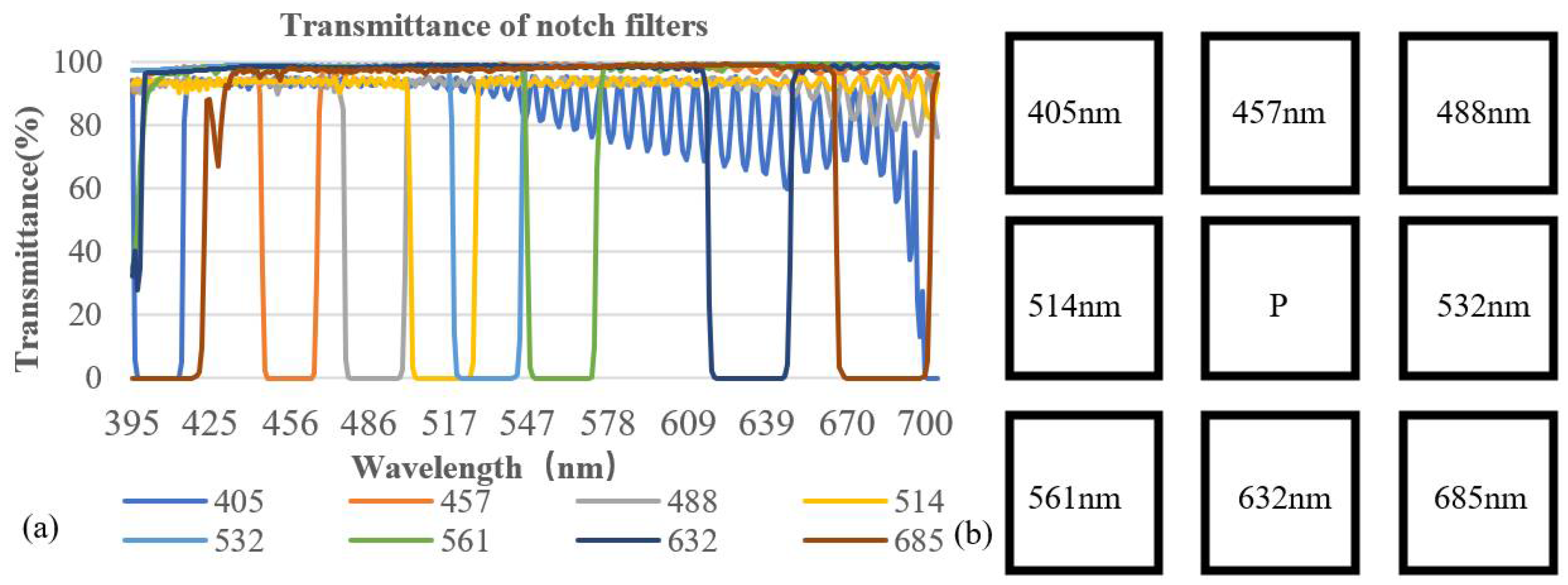
• A multispectral imaging system that combines a notch-filter array and multiple apertures is proposed. The use of notch filters enables the development of a high-light-efficiency imaging system that overcomes the drawbacks of conventional bandpass-filter-based multispectral imaging systems (e.g., low spatial resolutions and imaging speeds). Compared with CASSI or DCCHI systems, the proposed multi-aperture multispectral imaging system enables more spectral information from the target scene to be captured, significantly reducing the complexity of the underdetermined reconstruction problem. Compared with those of other bandpass-filter-based multispectral imaging systems, the higher light efficiency yielded by the notch-filter array significantly improves the imaging quality and temporal resolution of the multispectral imaging system.
• A dictionary learning- and TV-based spectral super-resolution algorithm (DL-TV) is proposed; it can train sparse dictionaries to achieve a high imaging quality as well as reduce noise with TV. Because the proposed method introduces more imaging priors, it can provide better imaging performance than the alternative direction multiplier method (ADMM) [32] with the dictionary learning algorithm (DL) [33].
• The effectiveness of the proposed system and algorithm is demonstrated through simulations using various datasets.
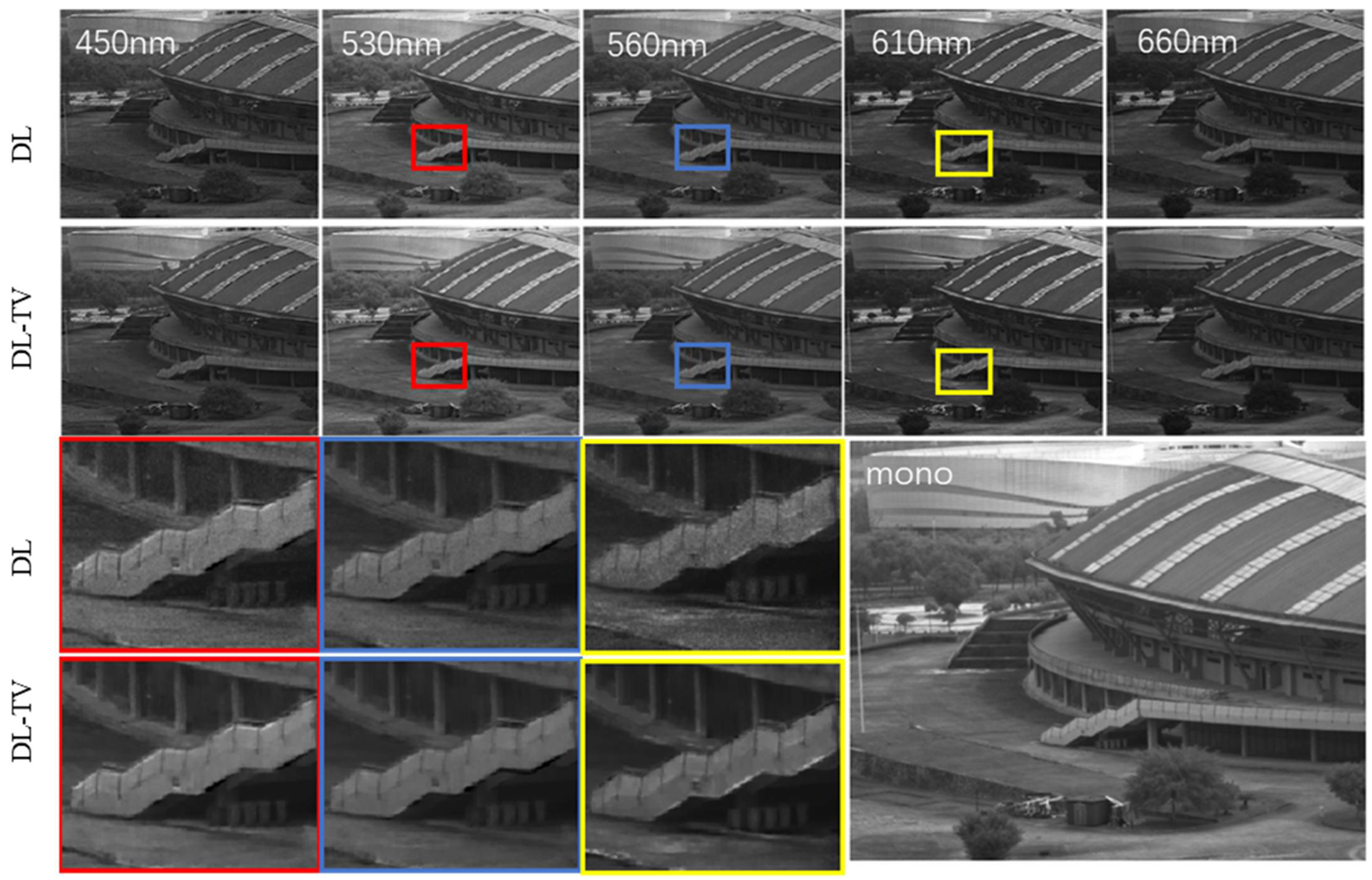
• A snapshot multispectral-imaging prototype system is built to verify real-world imaging performance via indoor experiments and field tests. The experimental results demonstrate that the combination of the proposed imaging system and compressive-sensing-based super-resolution spectral algorithm can obtain high-quality as well as high-spatial-spectral-resolution images.

2. Methods

2.1. Notch Filter Imaging Model

An MSI is a 3D data cube represented by $\mathit{C}\in {ℝ}^{M\times N\times Q}$, where $M$ and $N$ are the spatial dimensions of the image and $Q$ is the spectral dimension. Owing to the difficulty of mathematically modeling and constructing an optimization function for a 3D data block, $\mathit{C}$ is transformed into a 2D matrix: $\mathit{X}\in {ℝ}^{Q\times MN}$, where $MN$ represents the product of two spatial dimensions.

Figure 1 shows the spectral transmittance of the eight notch filters used in this study. The notch images, $\mathit{Y}\in {ℝ}^{K\times MN}$, captured by the notch filters can be expressed as:

$$\mathit{Y}=\mathit{T}\mathit{X},$$

(1)

where $\mathit{T}\in {ℝ}^{K\times Q}$ denotes the transmittance measurement matrix of the proposed system and is determined by the selected notch filters. For the simulation and experiments, $k=9$ was used. $\mathit{T}(i,\lambda )$ denotes the transmittance of the $i^{th}$ notch filter at the ${\lambda }^{th}$ band. Compared with a bandpass filter, which transmits only a narrow spectrum of light, resulting in a low light efficiency, the notch filter enables most of the spectrum to pass through while blocking only a specific portion of the spectrum. Consequently, the light efficiency of a notch-filter-based imaging system is close to that of a panchromatic imaging system. Therefore, the exposure time of the imaging process can be decreased, and the signal-to-noise ratio and imaging speed can be improved. For a notch-filtered spectral image, the corresponding bandpass spectral image was obtained by subtracting the panchromatic image from the notch-filtered spectral image. As shown in Figure 1, in the proposed multi-aperture multispectral imaging system, eight of the nine apertures were covered with a notch filter, and the central aperture was used to capture a panchromatic image.

In an ideal situation, the transmittances of the transmission and cutoff bands are 100% and 0%, respectively. Therefore, the transmittance in the ideal case can be approximately written as

$$\mathit{T}(i,\lambda )=\{\begin{array}{l}1,\hspace{1em}otherwise\\ 0,\hspace{1em}\left|\lambda -a_i\right|\le b_i\end{array},$$

(2)

where $a_i$ denotes the central wavelength of the $i^{th}$ notch filter, and $b_i$ is its corresponding full bandwidth at half maximum. However, owing to the optical materials and manufacturing errors, the actual transmittance of the transmission band is between 90% and 100%, whereas the cutoff transmittance is less than 10% [5].

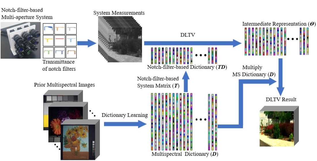
2.2. Spectral Super-Resolution Algorithm

Reportedly, the spectral information of one pixel can be sparsely represented by a trained dictionary [34], and the calculated results outperform the linear combination of a few spectral bases obtained via principal component analysis [35]. For a point $(m,n)$ on a spectral image, the spectral vector ${\mathit{x}}_j\in {ℝ}^{Q\times 1}$ can be expressed as

$${\mathit{x}}_j=\mathit{D}{\mathbf{\theta }}_j,j=\{1,\dots ,MN\},$$

(3)

where $\mathit{D}\in {ℝ}^{Q\times P}$ denotes an overcomplete dictionary trained using MSIs. $P$ is the number of dictionary atoms. Here, $Q=31$ and $P=2Q=62$. The dictionary $\mathit{D}$ was trained using the K-SVD algorithm by generalizing the K-means clustering process [36]. We let ${\mathbf{\theta }}_j\in {ℝ}^{P\times 1}$ denote the sparse vector of ${\mathit{x}}_j$ with a much smaller number (<Q) of nonzero elements. To speed up the calculation, all the pixels in the spatial domain were simultaneously calculated. Substituting Equation (3) into Equation (1) yields

$$\mathit{Y}=\mathit{T}\mathit{D}\mathit{\Theta },$$

(4)

where the sparse matrix, $\mathit{\Theta }\in {ℝ}^{P\times MN}$, must be solved, and its nonzero elements must be minimized as follows:

$$\underset{\mathit{\Theta }}{\arg \min }\frac{1}{2}{\Vert \mathit{Y}-\mathit{T}\mathit{D}\mathit{\Theta }\Vert }_{\mathrm{F}}^2+\eta {\Vert \mathit{\Theta }\Vert }_1.$$

(5)

The first term in Equation (5) is the fidelity term, the second term is the sparse term, and $\eta$ is the regularization factor that balances the fidelity and sparse terms. Because the MSIs are smooth in the spatial dimension, the TV constraint term [37] is added to the optimization objective of Equation (5) and can be expressed as:

$$\underset{\mathit{\Theta }}{\arg \min }\frac{1}{2}{\Vert \mathit{Y}-\mathit{T}\mathit{D}\mathit{\Theta }\Vert }_{\mathrm{F}}^2+\eta {\Vert \mathit{\Theta }\Vert }_1+{\eta }_{\mathrm{TV}}{\Vert \mathit{X}\Vert }_{\mathrm{TV}},$$

(6)

where ${\eta }_{\mathrm{TV}}$ is the regularization factor used to adjust the smoothness of the target, and ${\Vert \mathit{X}\Vert }_{\mathrm{TV}}$ is the TV constraint term, which can be expressed as:

$$\begin{array}{c}{\Vert \mathit{X}\Vert }_{\mathrm{TV}}={\displaystyle \sum _{\lambda =1}^Q{\displaystyle \sum _{m=1}^M{\displaystyle \sum _{n=1}^N\sqrt{{\mathit{X}}_{\mathrm{v}}{(\lambda ,(m-1)\times N+n)}^2+{\mathit{X}}_{\mathrm{h}}{(\lambda ,(m-1)\times N+n)}^2}}}}\\ \left[\begin{array}{c}{\mathit{X}}_{\mathrm{v}}(\lambda ,(m-1)\times N+n)\\ {\mathit{X}}_{\mathrm{h}}(\lambda ,(m-1)\times N+n)\end{array}\right]=\left[\begin{array}{l}\mathit{C}(m+1,n,\lambda )-\mathit{C}(m,n,\lambda )\\ \mathit{C}(m,n+1,\lambda )-\mathit{C}(m,n,\lambda )\end{array}\right],\end{array}$$

(7)

where ${\mathit{X}}_{\mathrm{v}}(\lambda ,(m-1)\times N+n)$ and ${\mathit{X}}_{\mathrm{h}}(\lambda ,(m-1)\times N+n)$ are the vertical and horizontal differences between the pixels of $\mathit{X}$, respectively. Substituting Equation (3) into Equation (6) yields

$$\underset{\mathit{\Theta }}{\arg \min }\frac{1}{2}{\Vert \mathit{Y}-\mathit{T}\mathit{D}\mathit{\Theta }\Vert }_F^2+\eta {\Vert \mathit{\Theta }\Vert }_1+{\eta }_{\mathrm{TV}}{\Vert \mathit{D}\mathit{\Theta }\Vert }_{\mathrm{TV}}.$$

(8)

By adding auxiliary variables ${\mathit{Z}}_1=\mathit{\Theta }$ and ${\mathit{Z}}_2=\mathit{D}\mathit{\Theta }$ to Equation (8), the above problem can be written as

$$\begin{array}{c}\underset{\mathit{\Theta }}{\arg \min }\frac{1}{2}{\Vert \mathit{Y}-\mathit{T}\mathit{D}\mathit{\Theta }\Vert }_{\mathrm{F}}^2+\eta {\Vert {\mathit{Z}}_1\Vert }_1+{\eta }_{\mathrm{TV}}{\Vert {\mathit{Z}}_2\Vert }_{\mathrm{TV}},\\ s.t.{\mathit{Z}}_1=\mathit{\Theta },{\mathit{Z}}_2=\mathit{D}\mathit{\Theta }.\end{array}$$

(9)

The corresponding augmented Lagrangian function is as follows:

$$\begin{array}{cc}\hfill ℒ(\mathit{\Theta },{\mathit{Z}}_1,{\mathit{Z}}_2,{\mathit{V}}_1,{\mathit{V}}_2)& =\frac{1}{2}{\Vert \mathit{Y}-\mathit{T}\mathit{D}\mathit{\Theta }\Vert }_{\mathrm{F}}^2+\eta {\Vert {\mathit{Z}}_1\Vert }_1+{\eta }_{\mathrm{TV}}{\Vert {\mathit{Z}}_2\Vert }_{\mathrm{TV}}+\hfill \\ & \frac{{\rho }_1}{2}{\Vert \mathit{\Theta }-{\mathit{Z}}_1+\frac{{\mathit{V}}_1}{{\rho }_1}\Vert }_{\mathrm{F}}^2+\frac{{\rho }_1}{2}{\Vert \mathit{D}\mathit{\Theta }-{\mathit{Z}}_2+\frac{{\mathit{V}}_2}{{\rho }_2}\Vert }_{\mathrm{F}}^2.\end{array}$$

(10)

where ${\mathit{V}}_1$ and ${\mathit{V}}_2$ are the Lagrange multipliers, and ${\rho }_1$ and ${\rho }_2$ and are the coefficients of the regular terms. ADMM theory [32] states that minimizing (6) is equivalent to iterating over the following steps until convergence:

$${\mathit{\Theta }}^{k+1}=\underset{\mathit{\Theta }}{\arg \min }ℒ(\mathit{\Theta },{\mathit{Z}}_1^k,{\mathit{Z}}_2^k,{\mathit{V}}_1^k,{\mathit{V}}_2^k),$$

(11)

$${\mathit{Z}}_1^{k+1}=\underset{{\mathit{Z}}_1}{\arg \min }ℒ({\mathit{\Theta }}_1^{k+1},{\mathit{Z}}_1,{\mathit{V}}_1^k),$$

(12)

$${\mathit{Z}}_2^{k+1}=\underset{{\mathit{Z}}_2}{\arg \min }ℒ({\mathit{\Theta }}_1^{k+1},{\mathit{Z}}_2,{\mathit{V}}_2^k),$$

(13)

The Lagrange multipliers are updated by

$${\mathit{V}}_1^{k+1}={\mathit{V}}_1^k+{\rho }_1({\mathit{\Theta }}^{k+1}-{\mathit{Z}}_1^{k+1}),$$

(14)

$${\mathit{V}}_2^{k+1}={\mathit{V}}_2^k+{\rho }_2(\mathit{D}{\mathit{\Theta }}^{k+1}-{\mathit{Z}}_2^{k+1}).$$

(15)

where $k$ denotes the number of iterations. Equation (11) can be solved as follows:

$${\mathit{\Theta }}^{k+1}=\underset{\mathit{\Theta }}{\arg \min }\frac{1}{2}{\Vert \mathit{Y}-\mathit{T}\mathit{D}\mathit{\Theta }\Vert }_{\mathrm{F}}^2+\frac{{\rho }_1}{2}{\Vert \mathit{\Theta }-{\mathit{Z}}_1^k+\frac{{\mathit{V}}_1^k}{{\rho }_1}\Vert }_{\mathrm{F}}^2+\frac{{\rho }_2}{2}{\Vert \mathit{D}\mathit{\Theta }-{\mathit{Z}}_2^k+\frac{{\mathit{V}}_2^k}{{\rho }_2}\Vert }_{\mathrm{F}}^2,$$

(16)

$${\mathit{\Theta }}^{k+1}={({\mathit{D}}^T{\mathit{T}}^T\mathit{T}\mathit{D}+{\rho }_{1}I+{\rho }_2{\mathit{D}}^T\mathit{D})}^{-1}\times \left[{\mathit{D}}^T{\mathit{T}}^T\mathit{Y}+{\rho }_1\left({\mathit{Z}}_1^k-\frac{{\mathit{V}}_1^k}{{\rho }_1}\right)+{\rho }_2\left({\mathit{Z}}_2^k-\frac{{\mathit{V}}_2^k}{{\rho }_2}\right)\right],$$

(17)

where $\mathit{I}$ is the identity matrix, and the superscript $T$ denotes the matrix transpose. Equation (12) is a typical lasso problem and can be solved as follows:

$${\mathit{Z}}_1^{k+1}=\underset{{\mathit{Z}}_1}{\arg \min }\frac{{\rho }_1}{2}{\Vert {\mathit{\Theta }}^{k+1}-{\mathit{Z}}_1+\frac{{\mathit{V}}_1^k}{{\rho }_1}\Vert }_{\mathrm{F}}^2+\eta {\Vert {\mathit{Z}}_1\Vert }_1,$$

(18)

$${\mathit{Z}}_1^{k+1}=soft\left({\mathit{\Theta }}^{k+1}+\frac{{\mathit{V}}_1^k}{{\rho }_1},\frac{\eta }{{\rho }_1}\right).$$

(19)

Here, $soft()$ is the well-known soft-thresholding operator [38]

$$soft(a,b)=\max (\left|a\right|-b,0)\odot \mathit{s}(a),$$

(20)

where $\mathit{s}$ is the signum function [39,40]. Equation (13) is equivalent to

$${\mathit{Z}}_2^{k+1}=\underset{{\mathit{Z}}_2}{\arg \min }\frac{{\rho }_2}{2}{\Vert {\mathit{\Theta }}^{k+1}-{\mathit{Z}}_2+\frac{{\mathit{V}}_2^k}{{\rho }_2}\Vert }_{\mathrm{F}}^2+{\eta }_{\mathrm{TV}}{\Vert {\mathit{Z}}_2\Vert }_{\mathrm{TV}},$$

(21)

Equation (21) is a simple TV denoising problem that can be solved using any TV algorithm; however, the fast gradient projection algorithms are generally recommended for solving this equation because of their quick convergence [41]. When ${\eta }_{\mathrm{TV}}=0$, the algorithm is the DL algorithm (Algorithm 1).

Algorithm 1: DL-TV for MSI Reconstruction

1: Input: $\mathit{T}$, $\mathit{D}$, ${\rho }_1>0$, ${\rho }_2>0$

2: Initialization: ${\mathit{Z}}_1$, ${\mathit{Z}}_2$, ${\mathit{V}}_1$, ${\mathit{V}}_2$, $\mathit{\Theta }$, $Ite{r}_{\max }$, $k=1$;

3: while $k\le Ite{r}_{\max }$ do

4: Update ${\mathit{\Theta }}^{k+1}$ via Equation (17)

5: Update ${\mathit{Z}}_1^{k+1}$ via Equation (19)

6: Update ${\mathit{Z}}_2^{k+1}$ via Equation (21)

7: Update ${\mathit{V}}_1^{k+1}$ via Equation (14)

8: Update ${\mathit{V}}_2^{k+1}$ via Equation. (15)

9: end while

10: Compute ${\mathit{\Theta }}^{k+2}$ via Equation (17)

Output: MSI $\mathit{X}=\mathit{D}\times {\mathit{\Theta }}^{k+2}$

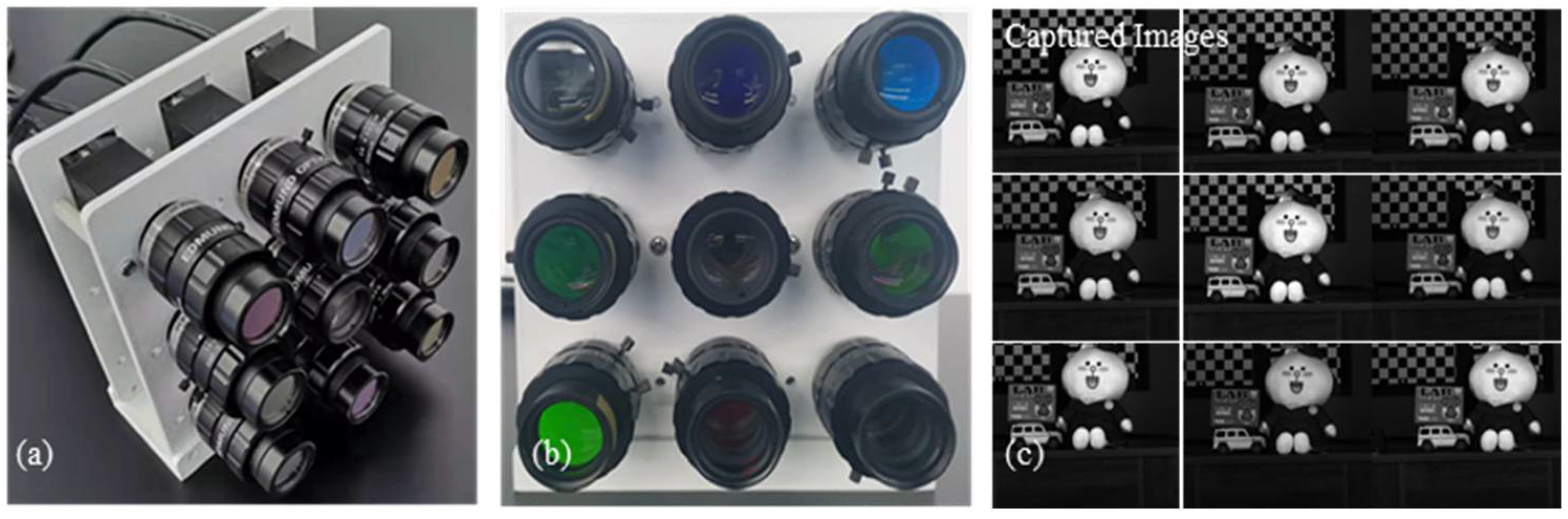
2.3. Prototype System

The proposed multi-aperture snapshot multispectral imaging system is shown in Figure 2. The system consists of an array of eight notch filters (Edmund OD 4.0 Notch), an array of lenses (Edmund FL 35 mm, f/1.8–f/16), and a monochromatic camera array (HIKVISION, MV-CA013-20GMGCGN). To record panchromatic images, no filter was added to the central lens, as shown in Figure 1b and Figure 2b. The eight surrounding lenses were equipped with notch filters of varying central wavelengths, as shown in Figure 1. All the cameras were synchronized to capture eight notch images and one panchromatic image simultaneously. Because the field of view of the images captured by each camera varies, image registration is required. The traditional bandpass multi-aperture system only captures a particular band of the spectrum of the target scenes. With most of the spectral bands missing, some areas of the spectral image appear dark, making the image registration of the multi-aperture image system difficult. The notch filter collects an image that is almost the same as a panchromatic image, because only a small portion of the spectrum is rejected, and the speeded up robust features algorithm can be used to achieve high-precision image registration [42].

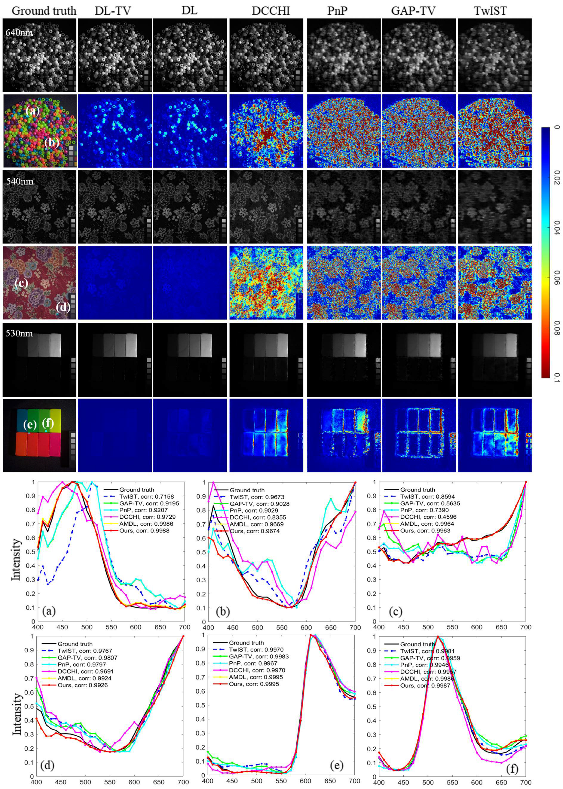
3. Simulations Using Public Datasets

The CAVE [43] and ICVL [44] datasets were used to verify the effectiveness of the proposed algorithm (Section 2). These datasets include MSIs with 31 spectral bands ranging from 400 to 700 nm, and the spectral resolution of the MSIs was 10 nm. The CAVE dataset includes 31 indoor MSIs with a spatial resolution of 512 × 512 pixels. The ICVL dataset includes 201 MSIs with a spatial resolution of 1392 × 1300 pixels, and downsampling to 512 × 512 pixels during simulation. In this study, 16,000 pixel vectors were selected from 16 MSIs of the CAVE dataset to form the training dataset, as suggested in [44], and the remaining 15 MSIs were used as the test dataset, as listed in

Table 1. Average peak signal-to-noise ratio (PSNR) and structural similarity index measure (SSIM) of the 15 reconstructed MSIs corresponding to the CAVE dataset.

MSI	PSNR						SSIM
	TwIST [30]	GAP-TV [29]	PnP [45]	DCCHI [15]	DL [33]	DL-TV	TwIST	GAP-TV	PnP	DCCHI	DL	DL-TV
Balloons	31.941	33.530	34.215	38.970	42.039	42.630	0.950	0.943	0.955	0.990	0.990	0.993
Beads	20.788	21.873	21.870	25.189	36.586	37.030	0.568	0.558	0.559	0.825	0.966	0.969
CD	29.616	31.975	31.522	34.483	32.686	32.785	0.927	0.912	0.907	0.971	0.973	0.977
Toy	23.956	24.774	24.997	34.044	42.618	43.103	0.805	0.791	0.822	0.964	0.991	0.995
Clay	31.954	32.979	32.960	36.754	44.938	46.720	0.907	0.893	0.897	0.952	0.976	0.984
Cloth	23.292	23.517	23.942	24.825	41.492	42.523	0.490	0.486	0.500	0.800	0.982	0.985
Egyptian	32.753	32.867	32.453	43.503	48.820	50.089	0.904	0.906	0.921	0.992	0.990	0.996
Face	32.467	32.449	32.463	40.814	44.153	44.975	0.928	0.915	0.908	0.988	0.985	0.994
Beers	30.190	32.127	34.265	39.194	42.037	42.456	0.940	0.928	0.952	0.984	0.991	0.995
Food	30.282	31.186	32.114	36.643	44.688	45.706	0.872	0.853	0.904	0.952	0.987	0.991
Lemon	28.853	29.733	30.695	39.833	47.357	48.458	0.871	0.841	0.874	0.975	0.991	0.994
Lemons	33.485	33.282	33.196	41.851	47.562	48.662	0.938	0.924	0.927	0.983	0.992	0.996
Peppers	28.501	30.187	30.621	36.307	44.854	45.744	0.893	0.893	0.908	0.950	0.989	0.993
Strawberries	32.089	31.353	30.832	41.738	47.019	48.065	0.895	0.870	0.887	0.971	0.991	0.994
Sushi	31.637	32.301	32.893	40.863	46.039	46.821	0.955	0.948	0.958	0.989	0.990	0.993
Average	29.454	30.275	30.603	37.001	43.526	44.384	0.856	0.844	0.859	0.952	0.986	0.990

. When choosing the training set, the central region of each image was sampled to avoid the black background area. For the trained dictionaries, different dictionaries resulted in different imaging qualities for each MSI in the test set. Therefore, all test sets shown in Section 3 as well as the field test data presented in Section 4 were implemented using the same dictionary trained in this study. In the simulation, eight notch images and one panchromatic image were created to simulate the images obtained using the proposed system. Because of the fast convergence of the ADMM algorithm, the number of DL-TV and DL iterations was set to $k=40$ in this study. When performing calculations using the CAVE and ICVL datasets, the parameters used in DL and DL-TV were set as follows: DL: $\eta =0.01$, $\rho =0.001$; DL-TV: $\eta =0.01$, ${\eta }_{\mathrm{TV}}=0.00001$, ${\rho }_1=0.001$, ${\rho }_2=0.001$.

For comparison, CASSI simulations were conducted using TwIST with the TV algorithm, GAP-TV, and the plug-and-play (PnP) approach [45], and the DCCHI simulations were performed using TwIST with the TV algorithm. The coded aperture mask reported in [45] was used for simulation. Zhang et al. [46] mentioned that TwIST would converge after 80 iterations; therefore, the iteration number in TwIST was set to 150. According to [14], the regularization parameter used in TwIST was set to τ = 0.1. The iterations and parameters of PnP and GAP-TV were set as reported in [45].

The test results are presented in Table 1,

Table 2. Average root-mean-square error (RMSE) and spectral angle mapper (SAM) of the 15 reconstructed MSIs corresponding to the CAVE dataset.

MSI	RMSE						SAM
	TwIST	GAP-TV	PnP	DCCHI	DL	DL-TV	TwIST	GAP-TV	PnP	DCCHI	DL	DL-TV
Balloons	6.483	5.387	4.974	2.914	2.644	2.560	0.091	0.085	0.119	0.070	0.088	0.085
Beads	23.518	20.702	20.709	14.366	4.877	4.738	0.304	0.311	0.310	0.313	0.109	0.104
CD	8.498	6.455	6.807	4.848	7.286	7.204	0.121	0.134	0.193	0.094	0.130	0.127
Toy	16.240	14.781	14.399	5.554	2.259	2.175	0.182	0.187	0.210	0.125	0.085	0.075
Clay	6.673	5.917	5.864	3.859	1.712	1.562	0.190	0.228	0.316	0.156	0.148	0.124
Cloth	17.631	17.118	16.405	15.964	3.032	2.878	0.171	0.172	0.171	0.318	0.081	0.080
Egyptian	5.934	5.832	6.103	1.716	1.172	1.084	0.264	0.255	0.347	0.113	0.172	0.140
Face	6.113	6.107	6.086	2.400	1.908	1.823	0.131	0.144	0.244	0.087	0.108	0.095
Beers	7.917	6.329	4.952	2.915	2.501	2.413	0.044	0.041	0.042	0.033	0.038	0.038
Food	7.893	7.080	6.331	3.812	1.979	1.888	0.154	0.181	0.213	0.137	0.120	0.113
Lemon	9.259	8.344	7.460	2.656	1.364	1.264	0.177	0.229	0.254	0.143	0.108	0.099
Lemons	5.421	5.539	5.605	2.090	1.315	1.224	0.107	0.117	0.217	0.087	0.082	0.073
Peppers	9.609	7.917	7.520	3.923	1.784	1.691	0.156	0.165	0.241	0.152	0.114	0.103
Strawberries	6.375	6.921	7.391	2.132	1.416	1.325	0.149	0.177	0.248	0.105	0.096	0.087
Sushi	6.701	6.216	5.796	2.350	1.715	1.644	0.106	0.126	0.184	0.080	0.138	0.130
Average	9.618	8.710	8.427	4.767	2.464	2.365	0.156	0.170	0.221	0.134	0.108	0.098

,

Table 3. Average PSNR and SSIM of the 15 reconstructed MSIs for the ICVL dataset.

MSI	PSNR						SSIM
	TwIST	GAP-TV	PnP	DCCHI	DL	DL-TV	TwIST	GAP-TV	PnP	DCCHI	DL	DL-TV
4cam1640	33.015	33.094	33.632	35.419	43.257	43.817	0.857	0.842	0.845	0.963	0.992	0.994
BGU1113	25.628	26.814	27.912	33.257	40.845	41.251	0.785	0.770	0.796	0.960	0.990	0.992
BGU1136	27.366	28.047	28.765	32.470	42.085	42.230	0.801	0.790	0.838	0.963	0.994	0.995
Flower1336	24.876	26.054	27.235	27.001	40.061	40.459	0.676	0.677	0.714	0.905	0.987	0.988
Labtest1502	31.674	30.418	29.901	40.858	48.608	49.425	0.879	0.841	0.849	0.982	0.996	0.997
Labtest1504	37.060	37.019	37.915	42.547	52.464	53.778	0.940	0.931	0.938	0.988	0.998	0.999
CAMP1659	27.165	28.585	29.365	35.412	39.474	39.738	0.863	0.853	0.850	0.977	0.993	0.995
bgu1459	31.275	31.042	31.788	37.235	45.490	46.376	0.831	0.819	0.833	0.968	0.989	0.990
bgu1523	25.717	26.944	27.325	28.526	39.883	40.109	0.763	0.754	0.798	0.930	0.988	0.989
eve1549	33.527	34.585	35.221	38.622	44.409	44.654	0.898	0.888	0.890	0.977	0.995	0.996
eve1602	28.396	28.515	28.957	31.834	41.213	41.325	0.823	0.802	0.833	0.951	0.991	0.993
gavyam0930	32.781	31.870	31.867	40.023	45.644	45.953	0.860	0.831	0.831	0.971	0.994	0.995
grf0949	27.403	27.865	28.849	30.452	42.080	42.655	0.746	0.737	0.761	0.934	0.989	0.992
hill1219	26.995	28.057	28.656	27.617	40.198	40.699	0.735	0.729	0.740	0.913	0.987	0.989
hill1235	28.370	29.203	29.651	28.408	39.655	40.144	0.771	0.767	0.769	0.932	0.988	0.992
Average	29.417	29.874	30.469	33.979	43.024	43.508	0.815	0.802	0.819	0.954	0.991	0.993

and

Table 4. Average RMSE and SAM of the 15 reconstructed MSIs for the ICVL dataset.

MSI	RMSE						SAM
	TwIST	GAP-TV	PnP	DCCHI	DL	DL-TV	TwIST	GAP-TV	PnP	DCCHI	DL	DL-TV
4cam1640	5.859	5.725	5.438	4.667	2.206	2.145	0.036	0.040	0.044	0.054	0.037	0.036
BGU1113	13.823	11.905	10.668	5.954	2.939	2.878	0.074	0.079	0.077	0.084	0.059	0.059
BGU1136	11.181	10.245	9.362	6.758	2.787	2.808	0.072	0.081	0.077	0.079	0.038	0.038
Flower1336	14.867	12.976	11.551	12.881	3.782	3.808	0.078	0.073	0.065	0.156	0.049	0.050
Labtest1502	6.810	7.726	8.181	2.365	1.137	1.072	0.047	0.067	0.066	0.034	0.032	0.031
Labtest1504	3.696	3.625	3.298	2.037	0.689	0.622	0.045	0.053	0.055	0.060	0.030	0.029
CAMP1659	11.262	9.612	8.931	4.793	3.874	3.888	0.056	0.053	0.054	0.050	0.040	0.041
bgu1459	7.307	7.280	6.788	3.712	1.992	1.930	0.075	0.092	0.092	0.078	0.068	0.067
bgu1523	13.244	11.537	11.000	10.660	3.832	3.875	0.069	0.061	0.064	0.130	0.055	0.056
eve1549	5.529	4.839	4.536	3.127	2.102	2.107	0.030	0.031	0.034	0.038	0.036	0.036
eve1602	9.775	9.594	9.108	7.201	3.095	3.109	0.040	0.048	0.054	0.074	0.042	0.042
gavyam0930	6.061	6.564	6.566	2.567	1.695	1.676	0.065	0.086	0.086	0.052	0.049	0.049
grf0949	11.263	10.514	9.548	8.421	2.752	2.692	0.062	0.063	0.061	0.112	0.046	0.045
hill1219	11.601	10.321	9.772	12.098	3.695	3.657	0.053	0.049	0.053	0.122	0.060	0.059
hill1235	9.963	9.050	8.695	11.065	3.583	3.500	0.040	0.037	0.043	0.100	0.050	0.050
Average	9.483	8.768	8.229	6.554	2.677	2.651	0.056	0.061	0.062	0.082	0.0461	0.0459

. Table 1 and Table 2 show the calculation results of the test dataset of 15 MSIs selected from the CAVE dataset, and Table 3 and Table 4 provide the calculation results for the ICVL dataset. For both the datasets and under all four metrics, DL outperformed TwIST, GAP-TV, PnP, and DCCHI, whereas DL-TV outperformed DL, demonstrating that DL-TV can effectively preserve the spectral information of the scene.

Figure 3 shows the simulation results generated from three different MSIs of the CAVE dataset. The spectral images reconstructed using DL-TV and DL were compared with those generated using the CASSI and DCCHI systems, and the corresponding error images were obtained from the reconstructed spectral image and ground-truth image for comparison. Spectral curves of selected regions were also plotted and compared with the ground truth. Additionally, the Pearson correlation coefficient (corr) was used to assess the fidelity of the recovered spectra. For the CASSI system, TwIST exhibited the poorest imaging quality, whereas GAP-TV and PnP provided slightly improved quality. Table 1, Table 2, Table 3 and Table 4 show that DCCHI can provide relatively better results than CASSI. The error images and spectral curves show that the combination of the proposed system and DL-TV significantly outperforms CASSI and DCCHI. It is clear that the imaging quality achievable by DL-TV is the best, so this approach yields accurate and detailed spectral textures of the target scene. Figure 4 shows the reconstructed spectra of “toy” MSI data. It can be clearly seen that DL-TV provides better reconstructed spectra than the other methods. Figure 5 plots three selected spectral frames from two ICVL scenes. Again, it is clear that DL-TV yields the best results.

In field tests, imaging noise is often introduced due to illumination conditions and imaging sensor noise. Hence, Gaussian noise with standard deviations of $\sigma =10,20,\mathrm{and}40$ was added during the simulation process for verification. Owing to the different noise levels, the regularization parameters must be tuned according to the noise level; in general, the larger the noise, the larger the regularization parameters.

Table 5. Average PSNR and SSIM of 15 reconstructed MSIs under different levels of noise, obtained using the CAVE dataset.

MSI	σ = 10				σ = 20				σ = 40
	PSNR		SSIM		PSNR		SSIM		PSNR		SSIM
	DL	DL-TV	DL	DL-TV	DL	DL-TV	DL	DL-TV	DL	DL-TV	DL	DL-TV
Balloons	32.637	36.647	0.742	0.919	29.309	34.079	0.543	0.863	25.480	30.981	0.354	0.683
Beads	30.328	31.114	0.824	0.878	27.932	28.613	0.695	0.816	24.670	27.262	0.544	0.720
CD	29.453	31.115	0.731	0.888	27.658	29.712	0.557	0.819	25.496	28.327	0.403	0.651
Toy	33.530	35.605	0.798	0.909	30.206	33.209	0.657	0.859	26.822	30.867	0.497	0.708
Clay	34.721	36.694	0.707	0.801	31.097	33.868	0.486	0.708	27.234	31.117	0.302	0.484
Cloth	32.940	34.669	0.783	0.872	28.887	31.574	0.614	0.810	24.802	29.130	0.451	0.683
Egyptian	36.571	40.108	0.821	0.898	32.932	37.568	0.638	0.813	29.332	33.529	0.426	0.593
Face	33.951	37.119	0.678	0.855	30.709	34.559	0.501	0.785	27.385	31.465	0.336	0.571
Beers	32.084	35.147	0.699	0.914	28.083	32.388	0.464	0.857	24.156	29.726	0.271	0.673
Food	34.614	35.535	0.790	0.879	30.727	32.965	0.614	0.822	26.909	30.446	0.442	0.661
Lemon	35.024	37.947	0.787	0.908	31.475	35.422	0.641	0.857	28.026	32.204	0.480	0.699
Lemons	34.905	37.766	0.756	0.886	31.032	35.076	0.571	0.823	27.301	31.842	0.406	0.649
Peppers	34.541	35.901	0.779	0.885	30.714	33.135	0.599	0.825	26.681	30.553	0.421	0.655
Strawberries	35.076	38.341	0.760	0.878	31.336	35.864	0.589	0.820	27.907	32.547	0.423	0.648
Sushi	36.024	38.328	0.786	0.899	32.274	36.061	0.621	0.843	29.242	32.731	0.466	0.668
Average	33.760	36.136	0.763	0.885	30.292	33.606	0.586	0.821	26.763	30.849	0.415	0.650

shows the simulation results for different levels of noise. It can be seen that irrespective of the noise level, the PSNR and SSIM of the spectral images generated by DL-TV are significantly higher than those of the images produced by DL, implying that DL-TV is more robust against noise. The algorithms were run on a Windows 10 64-bit system with AMD R5-4600H and 16 GB RAM, and the calculation time is shown in

Table 6. Comparison of reconstruction time in seconds between different methods.

Method	TwIST	GPA-TV	PnP	DCCHI	DL	DL-TV
Time	500.5	569.8	540.8	525.6	6.4	64.1

.

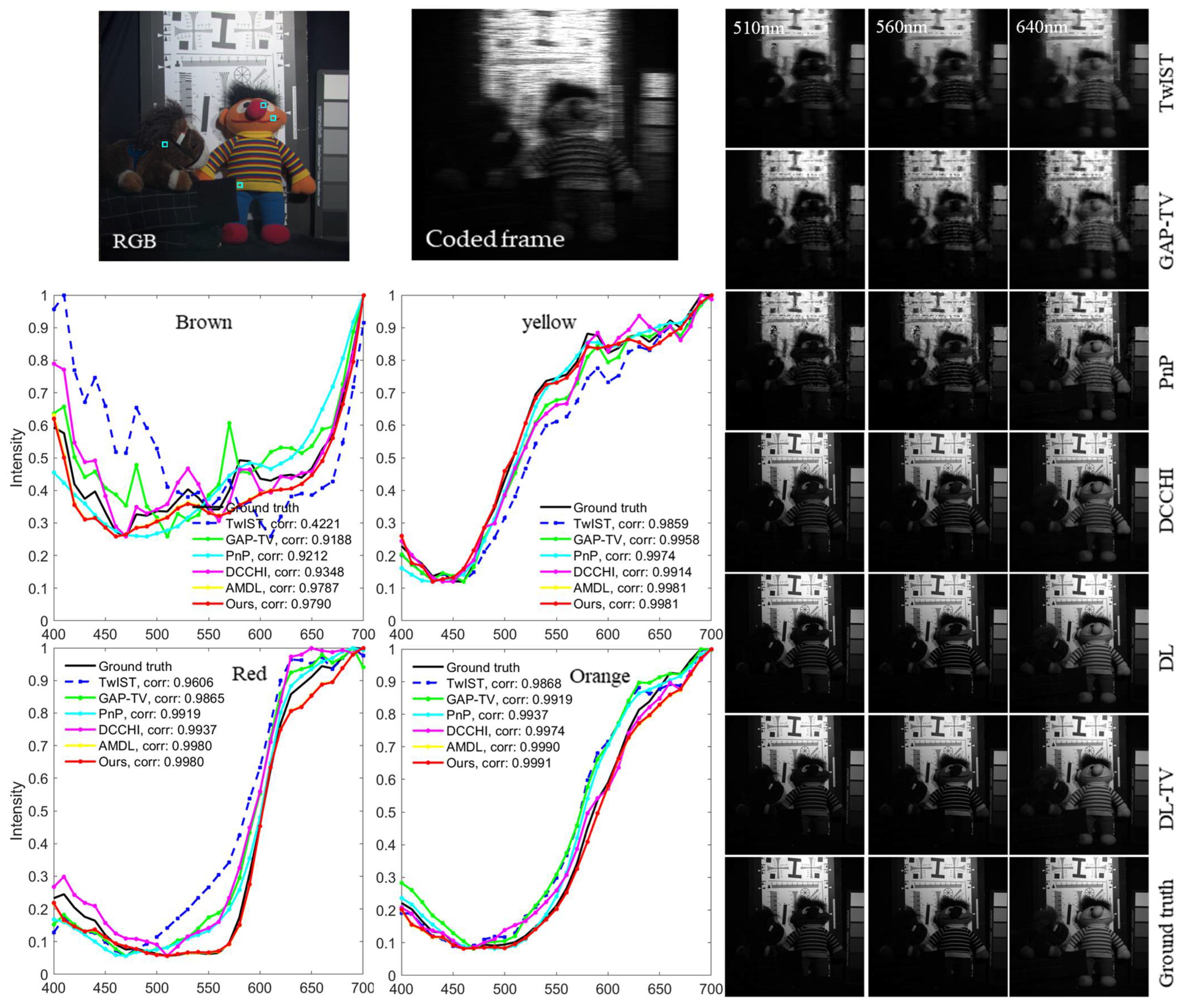
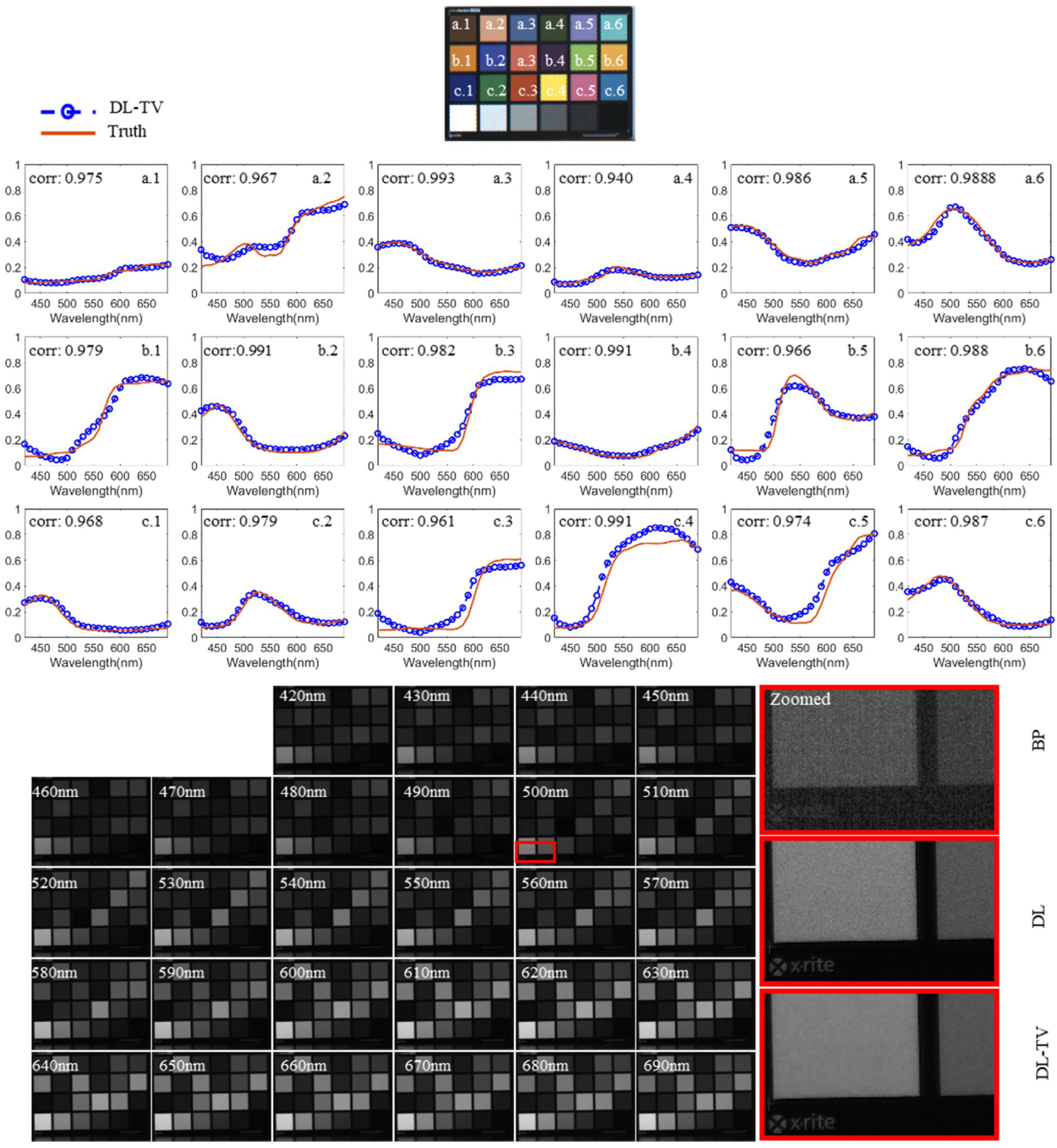
4. Experiments Using Actual Captured Data

4.1. Indoor Experiments

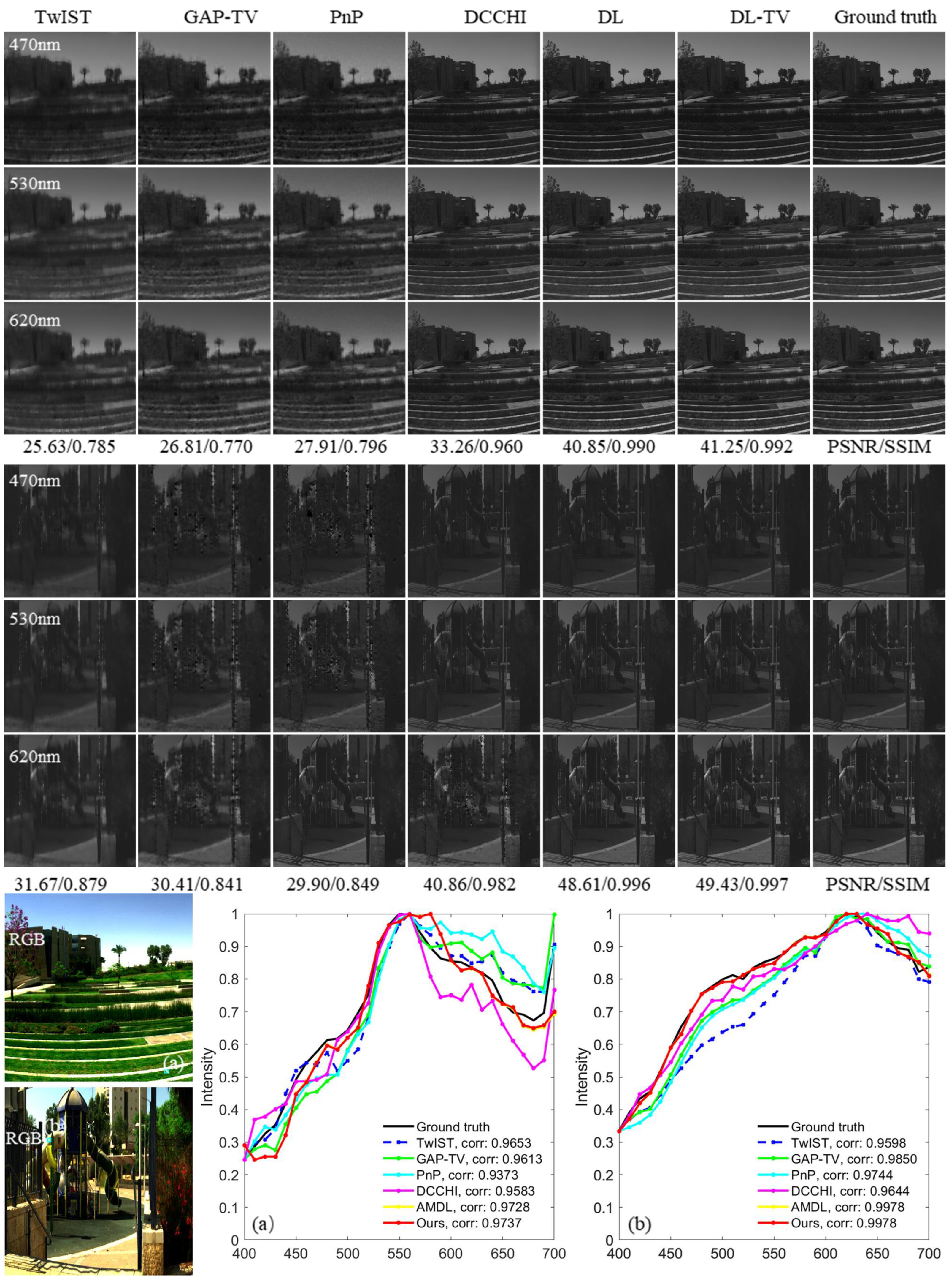
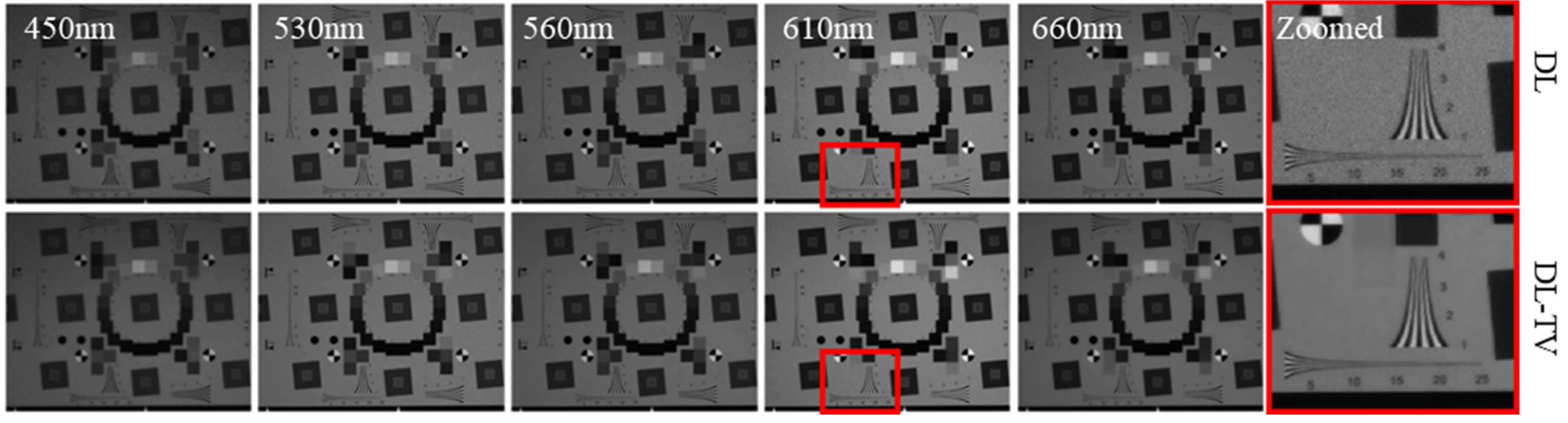
First, the notch-filter-based multi-aperture multispectral imaging system was built using nine monochromatic cameras, each with a resolution of 1024 × 1280 pixels, and this prototype system was used to capture the ColorChecker card and target image (ISO 12233 2014 eSFR) in an indoor environment. Eight notch-filtered images and one panchromatic image were collected in a single shot. The captured images were then processed using the proposed algorithms to reconstruct 31 bandpass spectral images. The illumination was provided by a spectrum-tunable light source (Thouslite-LEDCube) and was limited to the spectral range of 420–690 nm; therefore, the spectra of the MSIs in the experimental part also range from 420 to 690 nm, with the spectral bands of 28, as also reported in [47]. Figure 6 shows the reconstructed spectrum for 18 color blocks and the reconstructed MSIs for all bands. The exposure time for acquiring the notch-filtered and panchromatic images was 4 ms (frame rate of up to 250 fps). Simultaneously, the bandpass spectral images that were captured by the bandpass filters (THORLABS-FB) were obtained with the same exposure time. Figure 6 reveals that the calculated spectrum of the color block is almost the same as the ground truth captured by the hyperspectral camera (GaiaField_V10E), implying that the proposed system can restore the spectral information of the target scene. Figure 7 compares the hyperspectral images reconstructed by the proposed system with the DL and DL-TV algorithms. For demonstration, an ISO 12233 target was used along with the reconstructed spectral images with central wavelengths of 450, 530, 560, 610, and 660 nm, as shown in Figure 7. Figure 7 demonstrates that in the calculated spectral images, the detailed features and texture information of the ISO 12233 target are well preserved, indicating that the proposed system and algorithm do not reduce the spatial resolution of the target scene. In both scenes, it can be observed that compared to DL, DL-TV can effectively remove the noise from the actual captured data and can restore the target scene with higher accuracy. This experiment demonstrated the effectiveness of the prototype system and proposed algorithm for super-resolution spectral imaging.

4.2. Field Tests

For the field tests, the exposure time for capturing the notch-filtered and panchromatic images was set to 0.2 ms, and the theoretical frame rate of the imaging system was up to 5000 fps. For each single shot, the captured eight notch-filtered images and one panchromatic image were processed with DL-TV to generate 31 multispectral bandpass spectral images with central wavelengths in the range of 400–700 nm and a spectral resolution of 10 nm (i.e., at wavelengths of 400, 410, 420, 430, … 700 nm). Figure 8 shows 5 of the 31 reconstructed spectral images with central wavelengths of 450, 530, 560, 610, and 660 nm, along with a captured panchromatic image.

The field test results demonstrate that the proposed algorithm functioned efficiently for the prototype multispectral imaging system and could provide MSIs with a high frame rate.

5. Discussion

From Table 1, Table 2, Table 3 and Table 4, TwIST, GAP-TV, and PnP based on CASSI had lower PSNR, SSIM, and RMSE values for the CAVE and ICVL data sets than the DCHHI and the notch-multi-aperture system. On the MSIs “beads”, “toy”, and “cloth”, the CASSI reconstruction results had the worst PSNR, SSIM, and RMSE. As shown in Figure 3 and Figure 4, both “beads” and “cloth” had repetitive and complex texture structures. For “clay” with simple texture structure, it can be well reconstructed, as shown in rows 5 and 6 of Figure 3. The coded aperture broke the spatial structure of the scene (as shown in Figure 4); it therefore had difficulty retaining the texture information. DCCHI captured the panchromatic image and coded frame at the same time, obtaining more spatial-texture information than CASSI, so it achieved better PSNR, SSIM, and RMSE; however, its reconstruction–evaluation measurements on “beads” and “cloth” were not very good. The proposed notch-multi-aperture system obtained eight notch images and a panchromatic image at the same time, so it had more information about the target scene than CASSI and DCCHI; as a result, it achieved good evaluation indicators on all tested MSIs.

6. Conclusions

A multispectral imaging system that combines notch filters and multiple apertures is proposed. By taking advantage of the high light efficiency of the notch filters, the exposure time can be reduced to <0.2 ms under natural daylight. The proposed system was evaluated via simulations on the CAVE and ICVL datasets, and the corresponding results were compared with those obtained using the CASSI and DCCHI systems. Evidently, the proposed system can effectively improve imaging quality, and the proposed super-resolution spectral imaging methods provide better reconstruction quality and robustness against noise than those facilitated by the DL algorithm.

The proposed system can be used in medical contexts to capture the morphological and biochemical characteristics required for accurate disease diagnosis or functional analysis during a surgical operation. It is also suitable for dynamic remote-sensing classification, mineral analysis, and monitoring of agricultural produce.

Although the proposed system exhibits a high spatial quality and spectral fidelity, some of its aspects require further improvements. First, when capturing scenes with large depth differences, the registration accuracy of the images captured by different apertures is reduced, which could affect the quality of the reconstructed MSIs. Therefore, a better registration algorithm is required to expand the depth of field of the proposed system. Second, as the DL and DL-TV calculations for 512 × 512 × 31 MSI reconstruction are time-consuming, future work will be focused on developing a faster algorithm for real-time multispectral imaging. A deep learning algorithm could be used to replace the iterative process [48], which would greatly reduce the calculation time.

References

1. Landgrebe, D. The evolution of Landsat data analysis. Photogramm. Eng. Remote Sens. 1997, 63, 859–867. [Google Scholar]
2. Lu, G.; Fei, B. Medical hyperspectral imaging: A review. J. Biomed. Opt. 2014, 19, 010901. [Google Scholar] [CrossRef] [PubMed]
3. Wang, L.V.; Wu, H.-I. Biomedical Optics: Principles and Imaging; John Wiley & Sons: Hoboken, NJ, USA, 2012. [Google Scholar]
4. Gat, N.; Subramanian, S.; Barhen, J.; Toomarian, N. Spectral imaging applications: Remote sensing, environmental monitoring, medicine, military operations, factory automation, and manufacturing. In Proceedings of the 25th AIPR Workshop: Emerging Applications of Computer Vision, Washington, DC, USA, 16–18 October 1996; pp. 63–77. [Google Scholar]
5. Zhang, M.; Wang, L.; Zhang, L.; Huang, H. High light efficiency snapshot spectral imaging via spatial multiplexing and spectral mixing. Opt. Express 2020, 28, 19837–19850. [Google Scholar] [CrossRef] [PubMed]
6. Mu, T.; Han, F.; Bao, D.; Zhang, C.; Liang, R. Compact snapshot optically replicating and remapping imaging spectrometer (ORRIS) using a focal plane continuous variable filter. Opt. Lett. 2019, 44, 1281–1284. [Google Scholar] [CrossRef] [PubMed]
7. Liang, J.; Tian, X.; Ju, H.; Wang, D.; Wu, H.; Ren, L.; Liang, R. Reconfigurable snapshot polarimetric imaging technique through spectral-polarization filtering. Opt. Lett. 2019, 44, 4574–4577. [Google Scholar] [CrossRef] [PubMed]
8. Goetz, A.F.; Vane, G.; Solomon, J.E.; Rock, B.N. Imaging spectrometry for earth remote sensing. Science 1985, 228, 1147–1153. [Google Scholar] [CrossRef] [PubMed]
9. Sellar, R.G.; Boreman, G.D. Comparison of relative signal-to-noise ratios of different classes of imaging spectrometer. Appl. Opt. 2005, 44, 1614–1624. [Google Scholar] [CrossRef]
10. He, Q.; Wang, R. Hyperspectral imaging enabled by an unmodified smartphone for analyzing skin morphological features and monitoring hemodynamics. Biomed. Opt. Express 2020, 11, 895–910. [Google Scholar] [CrossRef]
11. Genser, N.; Seiler, J.; Kaup, A. Camera array for multi-spectral imaging. IEEE Trans. Image Process. 2020, 29, 9234–9249. [Google Scholar] [CrossRef]
12. Gehm, M.E.; John, R.; Brady, D.J.; Willett, R.M.; Schulz, T.J. Single-shot compressive spectral imaging with a dual-disperser architecture. Opt. Express 2007, 15, 14013–14027. [Google Scholar] [CrossRef]
13. Tao, C.; Zhu, H.; Sun, P.; Wu, R.; Zheng, Z. Hyperspectral image recovery based on fusion of coded aperture snapshot spectral imaging and RGB images by guided filtering. Opt. Commun. 2020, 458, 124804. [Google Scholar] [CrossRef]
14. Wang, L.; Xiong, Z.; Gao, D.; Shi, G.; Wu, F. Dual-camera design for coded aperture snapshot spectral imaging. Appl. Opt. 2015, 54, 848–858. [Google Scholar] [CrossRef] [Green Version]
15. Wang, L.; Xiong, Z.; Gao, D.; Shi, G.; Zeng, W.; Wu, F. High-speed hyperspectral video acquisition with a dual-camera architecture. In Proceedings of the IEEE Conference on Computer Vision and Pattern Recognition, Boston, MA, USA, 7–12 June 2015; pp. 4942–4950. [Google Scholar]
16. Wagadarikar, A.A.; Pitsianis, N.P.; Sun, X.; Brady, D.J. Video rate spectral imaging using a coded aperture snapshot spectral imager. Opt. Express 2009, 17, 6368–6388. [Google Scholar] [CrossRef] [PubMed]
17. Oiknine, Y.; August, I.; Stern, A. Multi-aperture snapshot compressive hyperspectral camera. Opt. Lett. 2018, 43, 5042. [Google Scholar] [CrossRef] [PubMed]
18. Carles, G.; Chen, S.; Bustin, N.; Downing, J.; McCall, D.; Wood, A.; Harvey, A.R. Multi-aperture foveated imaging. Opt. Lett. 2016, 41, 1869–1872. [Google Scholar] [CrossRef] [PubMed] [Green Version]
19. Candès, E.J.; Romberg, J.; Tao, T. Robust uncertainty principles: Exact signal reconstruction from highly incomplete frequency information. IEEE Trans. Inf. Theory 2006, 52, 489–509. [Google Scholar] [CrossRef] [Green Version]
20. Donoho, D.L. Compressed sensing. IEEE Trans. Inf. Theory 2006, 52, 1289–1306. [Google Scholar] [CrossRef]
21. Gan, L. Block compressed sensing of natural images. In Proceedings of the 15th International Conference on Digital Signal Processing, Cardiff, UK, 1–4 July 2007; pp. 403–406. [Google Scholar]
22. Fauvel, S.; Ward, R.K. An energy efficient compressed sensing framework for the compression of electroencephalogram signals. Sensors 2014, 14, 1474–1496. [Google Scholar] [CrossRef] [Green Version]
23. Leinonen, M.; Codreanu, M.; Juntti, M. Sequential compressed sensing with progressive signal reconstruction in wireless sensor networks. IEEE Trans. Wirel. Commun. 2014, 14, 1622–1635. [Google Scholar] [CrossRef]
24. Candes, E.; Romberg, J. Sparsity and incoherence in compressive sampling. Inverse Probl. 2007, 23, 969. [Google Scholar] [CrossRef] [Green Version]
25. Duarte, M.F.; Davenport, M.A.; Takhar, D.; Laska, J.N.; Sun, T.; Kelly, K.F.; Baraniuk, R.G. Single-pixel imaging via compressive sampling. IEEE Signal Process. Mag. 2008, 25, 83–91. [Google Scholar] [CrossRef] [Green Version]
26. Xue, J.; Zhao, Y.Q.; Bu, Y.; Liao, W.; Chan, J.C.W.; Philips, W. Spatial-spectral structured sparse low-rank representation for hyperspectral image super-resolution. IEEE Trans. Image Process. 2021, 30, 3084–3097. [Google Scholar] [CrossRef] [PubMed]
27. Llull, P.; Liao, X.; Yuan, X.; Yang, J.; Kittle, D.; Carin, L.; Sapiro, G.; Brady, D.J. Coded aperture compressive temporal imaging. Opt. Express 2013, 21, 10526–10545. [Google Scholar] [CrossRef] [PubMed] [Green Version]
28. Lustig, M.; Donoho, D.L.; Santos, J.M.; Pauly, J.M. Compressed Sensing MRI. IEEE Signal Process. Mag. 2008, 25, 72–82. [Google Scholar] [CrossRef]
29. Yuan, X. Generalized alternating projection based total variation minimization for compressive sensing. In Proceedings of the IEEE International Conference on Image Processing (ICIP), Phoenix, AZ, USA, 25–28 September 2016; pp. 2539–2543. [Google Scholar]
30. Bioucas-Dias, J.M.; Figueiredo, M.A. A new TwIST: Two-step iterative shrinkage/thresholding algorithms for image restoration. IEEE Trans. Image Process. 2007, 16, 2992–3004. [Google Scholar] [CrossRef] [Green Version]
31. Chambolle, A. An algorithm for total variation minimization and applications. J. Math. Imaging Vis. 2004, 20, 89–97. [Google Scholar]
32. Boyd, S.; Parikh, N.; Chu, E.; Peleato, B.; Eckstein, J. Distributed Optimization and Statistical Learning via the Alternating Direction Method of Multipliers. Found. Trends® Mach. Learn. 2011, 3, 1–122. [Google Scholar]
33. Huang, F.; Lin, P.; Wu, X.; Cao, R.; Zhou, B. Compressive Sensing-Based Super-Resolution Multispectral Imaging System. Available online: https://ui.adsabs.harvard.edu/abs/2022SPIE12169E..34H/abstract (accessed on 27 March 2022).
34. Lansel, S.; Parmar, M.; Wandell, B.A. Dictionaries for sparse representation and recovery of reflectances. In Proceedings of the IS&T-SPIE Electronic Imaging Symposium, San Jose, CA, USA, 19–20 January 2009. [Google Scholar]
35. Parkkinen, J.P.S.; Hallikainen, J.; Jaaskelainen, T. Characteristic spectra of Munsell colors. J. Opt. Soc. Am. A 1989, 6, 318–322. [Google Scholar] [CrossRef]
36. Aharon, M.; Elad, M.; Bruckstein, A. K-SVD: An algorithm for designing overcomplete dictionaries for sparse representation. IEEE Trans. Signal Process. 2006, 54, 4311–4322. [Google Scholar] [CrossRef]
37. Rudin, L.I.; Osher, S.; Fatemi, E. Nonlinear total variation based noise removal algorithms. Phys. D Nonlinear Phenom. 1992, 60, 259–268. [Google Scholar] [CrossRef]
38. Donoho, D.L. De-noising by soft-thresholding. IEEE Trans. Inf. Theory 1995, 41, 613–627. [Google Scholar] [CrossRef] [Green Version]
39. Yun, B.I.; Petković, M.S. Iterative methods based on the signum function approach for solving nonlinear equations. Numer. Algorithms 2009, 52, 649–662. [Google Scholar] [CrossRef]
40. Singh, D.; Kaur, M.; Jabarulla, M.Y.; Kumar, V.; Lee, H.-N. Evolving fusion-based visibility restoration model for hazy remote sensing images using dynamic differential evolution. IEEE Trans. Geosci. Remote Sens. 2022, 60, 1002214. [Google Scholar] [CrossRef]
41. Beck, A.; Teboulle, M. Fast gradient-based algorithms for constrained total variation image denoising and deblurring problems. IEEE Trans. Image Process. 2009, 18, 2419–2434. [Google Scholar] [CrossRef] [Green Version]
42. Bay, H.; Ess, A.; Tuytelaars, T.; Van Gool, L. Speeded-up robust features (SURF). Comput. Vis. Image Underst. 2008, 110, 346–359. [Google Scholar] [CrossRef]
43. Yasuma, F.; Mitsunaga, T. Generalized assorted pixel camera: Postcapture control of resolution, dynamic range, and spectrum. IEEE Trans. Image Process. 2010, 19, 2241–2253. [Google Scholar] [CrossRef] [Green Version]
44. Arad, B.; Ben-Shahar, O. Sparse recovery of hyperspectral signal from natural RGB images. In Proceedings of the European Conference on Computer Vision, Amsterdam, The Netherlands, 8–16 October 2016; pp. 19–34. [Google Scholar]
45. Zheng, S.; Liu, Y.; Meng, Z.; Qiao, M.; Tong, Z.; Yang, X.; Han, S.; Yuan, X. Deep plug-and-play priors for spectral snapshot compressive imaging. Photonics Res. 2021, 9, B18–B29. [Google Scholar] [CrossRef]
46. Zhang, S.; Huang, H.; Fu, Y. Fast parallel implementation of dual-camera compressive hyperspectral imaging system. IEEE Trans. Circuits Syst. Video Technol. 2018, 29, 3404–3414. [Google Scholar] [CrossRef]
47. Tao, C.; Zhu, H.; Wang, X.; Zheng, S.; Xie, Q.; Wang, C.; Wu, R.; Zheng, Z. Compressive single-pixel hyperspectral imaging using RGB sensors. Opt. Express 2021, 29, 11207–11220. [Google Scholar] [CrossRef]
48. Gregor, K.; LeCun, Y. Learning fast approximations of sparse coding. In Proceedings of the 27th International Conference on Machine Learning, Haifa, Israel, 21–25 June 2010; pp. 399–406. [Google Scholar]
Figure 1. (a) Transmittance of notch filters and (b) their locations in the multi-aperture imaging system. P indicates the aperture used for capturing panchromatic images. The central wavelengths of the notch filters are 405, 457, 488, 514, 532, 561, 632, and 685 nm.
Remotesensing 14 04115 g001
Figure 2. (a) Proposed multi-aperture multisystem, (b) lens array covered by the notch filter array shown in Figure 1b, and (c) images captured by the camera in (b) in a single shot.
Remotesensing 14 04115 g002
Figure 3. Simulation results calculated using three different MSIs of the CAVE dataset. The first, third, and fifth columns show the simulation results of “beads”, “cloth”, and “clay” MSIs. Error maps are shown in columns 2, 4, and 6 for comparison. To compare with the ground truth, the spectral curves of selected regions are shown in (af).
Remotesensing 14 04115 g003
Figure 4. Reconstruction spectra of “toy” MSI of the CAVE dataset. The original RGB image and the coded frame of the scene are shown at the top. The spectra of four color regions are shown on the left. The three reconstructed frames at wavelengths 510, 560, and 640 nm are shown on the right.
Remotesensing 14 04115 g004
Figure 5. Simulation results of “BGU1113” (top) and “Labtest1502” (bottom) MSIs of ICVL dataset. To compare with the ground truth, the spectral curves of selected regions are shown in (a,b).
Remotesensing 14 04115 g005
Figure 6. Comparison of the spectra of the 18 color blocks between the reconstructed results and ground truth. The reconstructed MSIs are displayed at the bottom. The spectral range is 420–700 nm. The zoomed-in regions for the 500 nm band are displayed in the right part. BP is the bandpass image.
Remotesensing 14 04115 g006
Figure 7. Comparison between the hyperspectral images reconstructed using the DL and DL-TV algorithms of the proposed system for the target image in the 450, 530, 560, 610, and 660 nm bands. Zoomed-in images for the 660 nm band are displayed as well.
Remotesensing 14 04115 g007
Figure 8. Field test results obtained by the proposed multispectral imaging system. The reconstructed MSIs were calculated using the DL and DL-TV algorithms. A total of 5 of the 31 reconstructed spectral images, with central wavelengths of 450, 530, 560, 610, and 660 nm, were selected and are shown. The zoomed-in regions from three selected spectral images are displayed, along with a captured monochromatic reference image.
Remotesensing 14 04115 g008