Abstract
Daily evapotranspiration (ET) integration is essential to various applications of agricultural water planning and management, ecohydrology, and energy balance studies. The constant reference evaporative fraction (EFr) temporal upscaling method has been proven to be efficient in extrapolating instantaneous ET to a daily timescale. Unlike upscaling methods, the direct calculation (DC) method developed in our previous study directly estimates daily ET without calculating instantaneous ET. The present study aimed to compare daily estimations of ET using the EFr and DC methods based on field and MODIS data at a site from the ChinaFLUX network. The estimation results were validated by eddy covariance (EC) ET both with and without the correction of energy imbalance. Based on field data, the results show that (i) the DC method performed with higher accuracy when compared to uncorrected EC measurements, while daily ET from both methods was overestimated; (ii) the DC method still performed better after the EC ET was corrected by the Residual Energy scheme, and the overestimations were significantly decreased; (iii) both methods performed best when compared with corrected ET by the Bowen Ratio scheme. The results from satellite data reveal that (i) the constant EFr method overestimated daily ET by a mean-bias-error (MBE) of 5.6 W/m2, and a root-mean-square error (RMSE) of 18.6 W/m2; and (ii) the DC method underestimated daily ET by a smaller MBE of −4.8 W/m2 and an RMSE of 22.5 W/m2. Therefore, the DC method has similar or better performance than the widely used constant EFr upscaling method and can estimate daily ET directly and effectively.
1. Introduction
Accurate estimation of actual evapotranspiration (ET) is urgently needed for a careful assessment of irrigation for agricultural production [1] and drought event monitoring [2], especially in regions characterized by water scarcity [3]. In these practical applications, there are still no specific ways to directly measure the actual ET. Conventional ET estimation techniques (i.e., pan-measures, Bowen ratio, eddy correlation system, and weighing lysimeter, scintillometer, sap flow) are mainly based on site scale and most of those techniques are of complexities [4]. Remote sensing observations from satellite sensors provide global coverage of critical land surface and atmospheric parameters; thus, ET retrieval models from remote sensing can be applied to quantify spatiotemporally continuous ET at regional or global scales [5,6].
Satellite images in different spectral ranges contain different information contents useful for estimating ET. Specifically, thermal images could provide the land surface temperature which is closely linked to the water status of the surface and therefore to ET; shortwave satellite images contain information on vegetation type and structure, which can be used in various ways to help quantify ET. Various models have been developed to utilize thermal and shortwave images for ET mapping [7]. The remotely sensed ET models available in the literature can be broadly classified as (1) fully physically based combination models that account for mass and energy conservation principles, including one-source [8,9] and two-source [10] ET models based on the surface energy balance, Penman–Monteith models [11], and canopy photosynthesis models [12]; (2) semi-physically based contextual models, such as the surface temperature–vegetation index triangle/trapezoid space based models [13,14]; and (3) black-box models based on artificial neural networks [15], empirical relationships [16], and fuzzy and genetic algorithms [17]. Based on these models, some ET products have been developed. For example, based on Penman–Monteith models and Moderate-resolution Imaging Spectroradiometer (MODIS) data, global ET product MOD16A2 with temporal and spatial resolution of 8 days and 1 km has been publicly accessible and widely applied for providing ET with high accuracy in the absence of flux towers, eddy covariance, and lysimeters [18,19].
Among these remotely sensed ET models, Penman–Monteith models and canopy photosynthesis models rely on shortwave remote sensing and meteorological data [20], and can provide instantaneous (half hour or an hour) and daily ET consistent with the timescale of input meteorological parameters. However, complex parameterizations of stomatal conductance usually limit their applications. The energy-balance-based single-source and two-source models, and triangle/trapezoid space-based models, which are the most widely applied ET models, generally rely on the radiometric temperature obtained from thermal remote sensing at the satellite scanning time. Therefore, most of these satellite models usually directly generate instantaneous ET values [7], while ET models containing more information with longer time scales (e.g., days, months, or years) play a more crucial role in practical applications, for example, agricultural water planning and management, ecohydrology, and energy balance studies [1,2,3].
For daily ET estimations, temporal upscaling is a common means through which instantaneous ET retrievals from satellite data are extrapolated to obtain more useful daily values. To date, a large range of temporal upscaling approaches has been developed and tested [21,22,23,24]. In these widely applied temporal upscaling approaches, the instantaneous ET is typically first retrieved and then extrapolated to obtain daily ET by assuming a constant proportion of ET to a given reference variable on a diurnal day. The accuracy of daily ET estimation is thus determined by the performance of the temporal upscaling approach itself, as well as the instantaneous ET calculation. The performances of these ET upscaling methods have been evaluated by some other previous studies [25,26,27,28,29]. Consistent conclusions have rarely been drawn, primarily because these comparisons differ in the utilization of modeled or observed fluxes as the upscaling proportions, in the upscaling of instantaneous ET to daytime or daily integrated values, and in the application of the upscaling methods under very limited conditions [30]. The constant reference evaporative fraction (EFr, a fraction in which the numerator is the actual ET and the denominator is the reference grass/alfalfa ET) method is one type of temporal upscaling approach [31]. In this method, EFr is assumed to remain relatively constant on a diurnal day, and daily ET is obtained after calculating the daily reference ET and the remotely sensed instantaneous ET. The constant EFr method has obvious advantages in incorporating the advective effect and reflecting the diurnal variations in net radiation, air temperature, wind speed, and relative humidity [32,33]. A large number of studies have deeply investigated the effectiveness and performance of this upscaling method, and its higher accuracy has been revealed by comparison with other methods [34,35].
Unlike the upscaling procedure, some daily ET calculation models were built by incorporating some parameters (e.g., solar radiation, relative humidity, air temperature, and wind speed) with several soft computing techniques and the combinations of them, e.g., the multilayer perceptron, support vector regression, and multilinear regression [36,37]. However, these models are usually weak in understanding the mechanism of ET process and their accuracies are closely related to the sample choices. The direct calculation (DC) method proposed in our previous study by a derivation of the physical-mechanism-based Penman–Monteith equation [38] can directly estimate daily ET, benefiting from the consistency of a decoupling coefficient (Ω). In the DC method, weather effects that influence the ET process are assumed from the available radiation and the interaction of the surface and atmosphere, and the degree of the interaction is depicted with the decoupling coefficient. Because the interaction between the atmosphere and vegetation does not change significantly during the same day, Ω is always assumed to be constant on a diurnal day, especially under clear conditions [39]. Therefore, the decoupling coefficient resulting from satellite data is intended to be applied in the direct calculation of daily ET, and instantaneous ET is not the necessary input in this method. In our previous study [38], the DC method was validated only with measured ET values and lacks a comprehensive comparison with other methods.
It is apparent that the DC method is theoretically derived from the physics-based Penman–Monteith equation. Similarly, daily reference ET values calculated using the Penman–Monteith equation are the main inputs of the constant EFr method to accurately estimate daily ET [31]. Both the DC and constant EFr methods are solid physics-based methods that require similar ground-based meteorological variables (air temperature, vapor pressure deficit, and wind speed). Therefore, it is essential to compare the DC method and the widely used EFr method for cases in which they are driven with the same inputs, to provide scientific guidance for the development and application of a practical daily ET estimation method with high accuracy.
The objective of this study was twofold: (1) to estimate daily ET by direct calculation using the DC method and by temporal upscaling with the constant EFr method; (2) to evaluate the performances of these two estimation procedures. The estimation and evaluation were based on field data and remote sensing images collected at the Yucheng station in China. The test period was from late April 2009 to late October 2010. Validation of daily ET estimations was conducted on both closed and un-closed eddy covariance (EC) ET measurements to consider the effect of energy imbalance. Section 2 examines the basic theories of the DC method, constant EFr method, and methodology for the calculation of instantaneous ET required by the constant EFr method. Section 3 introduces the required meteorological variables, ET measurements, other energy flux data, and remote-sensing datasets, and presents the techniques for energy imbalance correction. Section 4 focuses on the estimation and evaluation results. Section 5 discusses the comparison and uncertainties of the estimation and evaluation. Finally, Section 6 provides the summary and conclusions.
2. Methodology
The daily ET in this study was estimated by direct calculation with the DC method and by temporal upscaling with the constant EFr method, using field data only at first to separate the satellite parameter retrieval errors, and then again with remote sensing data. Daily ET was directly calculated using the DC method and estimated by extrapolating the instantaneous ET through the constant EFr method, after calculation of the necessary satellite-based elements, including the land surface temperature (Ts), surface net radiation (Rn), and the soil heat flux (G).
2.1. Direct Calculation Method
The DC method was developed by rearranging the decoupling model which calculates ET by considering the relative contribution of the radiative (ETrad) and aerodynamic (ETaero) terms to the overall ET with a decoupling coefficient connecting the equilibrium evapotranspiration (ETeq) and imposed evapotranspiration (ETim) by the surrounding air [39]:
where ETrad is the thermodynamic ET in which the energy is from the radiative energy (W/m2); ETaero is the aerodynamic ET which is decided by the aerodynamic factors (e.g., vapor pressure) (W/m2); ETeq is the equilibrium, or radiation-controlled ET (W/m2); ETim is the imposed, or stomatal-controlled ET (W/m2); Rn is the surface net radiation (W/m2); G is the soil heat flux (W/m2); VPD is the vapor pressure deficit of the air (kPa); is the ratio of vapor pressure and air temperature (kPa/°C); γ is the psychrometric constant (kPa/°C); λ is the latent heat of vaporization here taken as 2.45 MJ kg−1; is the air density (kg/m3); Cp is the specific heat at constant pressure (J/(m·K)); and rs is the surface resistance (s/m).
The decoupling coefficient (Ω) connects the equilibrium evapotranspiration (ETeq) and imposed evapotranspiration (ETim) according to the coupling of the surface atmosphere. It varies between the values ‘0’ and ‘1’, with 0 reflecting a perfect coupling in which the atmosphere provides all the energy for the ET while value 1 reflecting a perfect decoupling condition in which the radiation provides all the energy. Ω was calculated from remote sensing data based on its relationship with the crop water stress index (CWSI) [40]:
where Ts is the land surface temperature (K) and Ta is the air temperature (K).
The theoretical minimum and maximum values for (Ts − Ta) are computed based on the energy balance equation by assuming two extreme surface conditions: extremely dry and extremely wet. Under extremely dry conditions, all the available energy (Rn − G) is utilized to heat the surface [Hdry = ρCp(Ts − Ta)/ra = (Rn − G)]; the ET is almost zero and rs is large enough; and (Ts − Ta) reaches its maximum; otherwise, under extremely wet conditions, rs approaches zero and (Ts − Ta) reaches its minimum. Based on this, the theoretical minimum, and maximum values for (Ts − Ta) were computed with inputs of Rn, G, aerodynamic resistance (ra, s/m), rs, and (ea* − ea), where ea* is the saturated vapor pressure at the evaporating front based on the air temperature (kPa); ea is the vapor pressure of the air above the canopy (kPa).
Considering that the decoupling coefficient resulted from satellite data is intended to replace daily values, daily ET is calculated based on Equation (1) after calculations of related ETeq and ETim based on Equations (2) and (3), using the decoupling coefficient combining them.
2.2. Constant EFr Temporal Upscaling Method
The constant EFr method assumes EFr (the ratio of actual ET to the reference evapotranspiration (ETr) expressed with Formula (8)) to be constant on a diurnal day, and daily ET in this method can be obtained after calculating the daily reference ET,
where the subscript i denotes the instantaneous scale at the satellite overpass and d denotes the daily scale.
The ETr at the instantaneous and daily scales was estimated from the Penman–Monteith equation [41], which was used to calculate ET for a hypothetical reference grass with a height of 0.12 m. The surface resistance was assumed to be 50 s/m during the daytime and 200 s/m during the nighttime. The assumed albedo is 0.23. ETr is expressed as follows:
where u2 is the wind speed at a height of 2 m (m/s); Cn has different values at the daily and hourly time scales of 900 and 37, respectively [41]; Cd equals different values at daytime and nighttime, 0.24 and 0.96, respectively [41]; and the remaining variables have the same definitions as those presented in the DC method.
The instantaneous ET required in the constant EFr method is calculated using Equation (11), with ra and rs computed by combining three equations (Equations (12)–(14)). A detailed description of the theory and procedure can be found in previous studies [42].
2.3. Retrievals of Satellite-Based Ts, Rn, and G
In this study, MODIS land surface temperature product (MOD11_L2) was utilized directly to provide land surface temperature (Ts, K) [43], which is used as a parameter for the calculation of the decoupling coefficient (Ω) in Equation (4) and satellite-based surface net radiation. The surface net radiation is the sum of the downward and upward shortwave and longwave radiation at the ground:
where Rg and Ru are the downward and upward shortwave radiations, respectively, W/m2; Ld and Lu are the downward and upward longwave radiations, respectively, W/m2; is the surface emissivity; is the atmospheric emissivity; and is the Stefan–Boltzmann constant. is the surface albedo retrieved with an empirical regression equation using MODIS surface reflectance products with band 5 removed (the subscript is the number of bands) [44]:
The retrieval of pixel-by-pixel soil heat flux was conducted through a semi-empirical formula in which the normalized difference vegetation index (NDVI) and surface temperature (Ts) products were applied to calculate the ratio of G to Rn:
2.4. Evaluation Metrics
The DC and constant EFr methods for daily ET estimations were evaluated based on both field measurements and satellite data by comparing daily ET estimations and observations, with some statistical items (MBE, RMSE, MAD, and R2, defined as follows) revealing their performances. Specifically, MBE is the mean-bias-error of the estimated data compared to the observed one, which is the amount of estimation bias with positive and negative values indicating higher and lower estimations, respectively; RMSE is the root-mean-square error from the comparison of estimated and observed daily ET; MAD is the mean-absolute difference from the comparison of estimated and observed values; and R2 is the determination coefficient of the regression relationship between the estimated and measured quantities,
where n is the number of test data; ESTi and OBSi are the daily ET estimations and observations; and are the average values for the ESTi and OBSi, respectively.
3. Materials
Daily ET estimations by direct calculation with the DC method and by temporal upscaling with the constant EFr method were conducted with climatic and satellite data at the Yucheng experimental station in China. The validation of daily ET estimations was implemented on both closed and un-closed EC ET measurements to consider the effect of energy imbalance. A flowchart describing the estimation and validation procedures is shown in Figure 1.
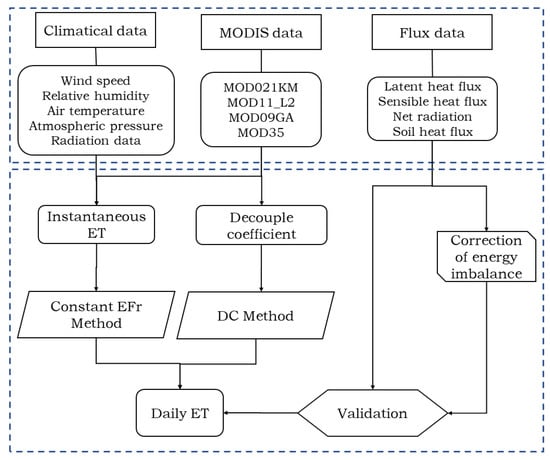
Figure 1.
Flowchart of daily ET estimation and validation procedures through the DC method and the constant EFr method.
3.1. Experimental Site
The Yucheng experimental site (longitude 116°22′–116°45′E and latitude 36°40′–37°12′N) is located in the southwest of Yucheng city, Shandong Province, China (Figure 2). This experimental site belongs to ChinaFLUX (Chinese Terrestrial Ecosystem Flux Research Network) aimed at the rational utilization of natural resources, such as climate, biology, soil, and water, and sustainable regional development. Through long-term accumulation of observations, data from the site provides measurements of the exchange of energy, heat, and water between the atmosphere and the land. The climate at this site can be characterized by a subhumid monsoon climate. The mean annual precipitation and temperature are 528 mm and 13.1 °C, respectively. The soil type is mainly sandy loam.
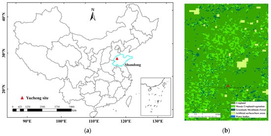
Figure 2.
Location map of the Yucheng experimental site (a) and land cover classification near the Yucheng site in 2009 from Global Land Cover Map in Google Earth Engine (b) (Yuchen site was indicated by the filled red triangle and Shandong province was labeled as light blue).
The crops in the study area are mainly rotated winter wheat and summer corn. The winter wheat was sown in late October and then harvested in mid-June; and the summer corn was planted in mid-June and matured and harvested in late September. Approximately 60–70% of the rainfall occurs in the summer corn growing season and the remaining 30–40% occurs in the winter wheat season. The flux measurements and climate variables collected in this study were from April 2009 to November 2010, covering a wide range of canopy coverage and water availability. All the meteorological variables and EC measurements were made in an experimental area approximately 250 m by 90 m. Vegetation height and leaf area index (LAI) in the experimental area were measured periodically every 15 and 7–8 days during the winter wheat and summer corn growth period. The experimental area has the same crop type as the surrounding farmland and is relatively uniform (Figure 2b).
3.2. Climatical and Flux Datasets
3.2.1. Climatical and Radiation Variables
The climatic variables tested in this study included the routinely measured wind speed, relative humidity, air temperature, and atmospheric pressure. These measurements were conducted at two levels: ~4.2 m in late July to early August at the corn stage and ~2.9 m in late October or early November at the wheat stage. Radiation measurements, including downwelling and upwelling shortwave and longwave radiation, were observed with Kipp and Zonen1 CNR-1 4-component net radiometers. The soil heat flux was measured with the vicinity of each lysimeter. The climatic and radiation measurements mentioned above were all half-hourly scales. Note that the climatic and radiation inputs for the DC and constant EFr methods primarily include air temperature, slope of vapor pressure, surface available energy, vapor pressure deficit (VPD), and wind speed at half-hourly and daily scales (average of 48 half-hourly measurements on a diurnal day).
3.2.2. Eddy Covariance Flux Measurements
The sensible heat flux (H) and latent heat flux (LE, energy expression of ET) used in this study were measured regularly using an EC system, which mainly included an open-path CO2/H2O gas analyzer (model LI-7500, Licor Inc., Lincoln, NE, USA) and a 3-D sonic anemometer/thermometer (model CSAT3, Campbell Scientific Inc., Logan, UT, USA). The measurement heights above the ground surface coincided with those of the climatic data. To measure these raw fluxes using the EC technique requires extensive data processing; thus, the measurements were checked with standard tools available in an open-source environment for processing high-frequency (10 or 20 Hz) data into half-hourly quality-checked fluxes with stationarity tests on covariances, flux calculations, and instrumental noise removal with conversions and corrections [45]. A series of data quality control procedures were performed to obtain a reliable EC-measured sensible heat flux and latent heat flux. In addition, according to the lower and upper limits of abnormalities, data spikes, and surface available energy, less than −100 W/m2 or greater than 700 W/m2 of these flux data were removed. The time scale of the flux data was one half-hour, which is consistent with that of climatic variables.
The EC-measured surface energy components are reported to have energy imbalance errors (namely, Rn − G > LE + H) owing to advection and soil heat storage [46]. To understand the effect of energy imbalance from the EC-measured surface energy and evaluate the daily ET estimations in these two ET estimation methods effectively, it is necessary to consider the energy imbalance of the EC-measured flux during the evaluation process. Two main schemes have been developed and widely utilized to correct the unclosed energy flux: the residual energy (RE) correction scheme and Bowen ratio (BR) correction scheme [47]. In the RE scheme, H is assumed to be measured correctly and the imbalanced energy is assigned to LE [Lec = (Rn − G) − H]. In the BR scheme, the BR is assumed to be measured correctly, and the surface available energy is repartitioned into H and LE according to the original EC-measured BR [LEc = LE/(H + LE)(Rn − G)]. Because there is no consensus on which correction scheme performs better, in this study, both methods were utilized to correct the half-hourly and daily EC measurements.
After quality-controlled and energy imbalance correction steps, daily ET measurements by the EC averaged from 0:00 h to 24:00 h local time with and without correction for energy imbalance were applied to validate and evaluate daily ET resulting from the DC and constant EFr methods.
3.3. Satellite Data
Satellite data tested in this study were obtained from the onboard MODIS sensor, including the MODIS Level 1 B Calibrated Radiances 1 km product (MOD021KM), MODIS/Terra Land Surface Temperature/Emissivity 5-Minute L2 Swath 1 km product (MOD11_L2), MODIS/Terra Surface Reflectance Daily L2G Global 1 km and 500 m SIN Grid product (MOD09GA), MODIS/Terra Geolocation Fields 5Min L1A Swath 1 km product (MOD03), and MODIS/Terra Cloud Mask and Spectral Test Results 5-Min L2 Swath 1 km product (MOD35).
The MOD021KM was applied to estimate the surface net radiation (Rn). The MOD11_L2 swath product was used to determine the land surface temperature (Ts). The surface reflectance of spectral bands 1 through 7 from MOD09GA was employed to estimate the surface albedo and then the NDVI with the spectral reflectance in the red and near-infrared bands. The MOD03 product contains information on geodetic coordinates (latitude and longitude), solar zenith and azimuth angles, satellite zenith and azimuth angles, and ground elevation for each 1 km pixel, which was used for the geo-calibration of all MODIS data in this study. MOD35 was applied to select a clear sky day together with the measured solar radiation.
3.4. Clear-Sky Selections and Energy Flux Correction
To derive the required inputs for instantaneous ET estimation, clear-sky days were selected for better satellite data quality, and the days when data gaps occurred because of rainfall events and instrument malfunction or maintenance were removed. Clear-sky day selection was constrained by cloud conditions at the satellite overpass time and measured downwelling shortwave radiation [48]. Finally, 45 clear-sky days were selected with a maximum gap of 83 days and average gaps of 13 days, referring to two successive MODIS images.
To reveal the necessity of the energy imbalance correction, the variations in Rn measurements, the EC measured LE with (the RE and BR corrections) and without correction of energy imbalance over 45 selected clear-sky days at 10:30 (corresponding to MODIS overpass time, recorded as instantaneous time), and daily scale are examined in Figure 3. For these selected days, the EC-measured LE at the 10:30 and daily scales were both considered as the largest energy component of the net radiation, and the measured LE closely followed the variation in the net radiation. Furthermore, the undermeasurements of LE at both instantaneous and daily scales were obvious. The closure ratio, which was used to reflect the degree of energy imbalance (defined as the ratio of the sum of H and LE to the surface available energy), averagely approximated 0.71 and 0.78 over the selected 45 days at the half-hourly and daily time scales, respectively.
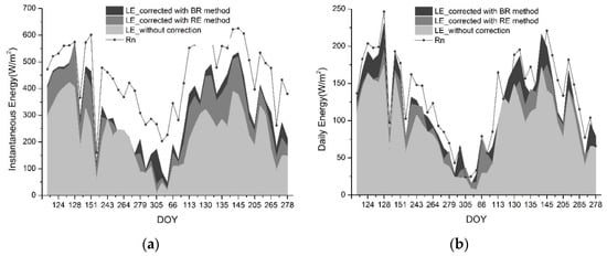
Figure 3.
Time-series of LE and Rn observations with and without energy imbalance corrections over the Yucheng site at (a) the instantaneous 10:30 scale and (b) the daily scale over 45 clear skies.
4. Results and Analysis
4.1. Evaluation Based on Field Data
4.1.1. Evaluation with Original Flux Measurements
Before the evaluation of daily ET estimations, instantaneous ETs of 45 selected clear days at 10:30 MODIS overpass time were estimated after the calculations of the related parameters based on meteorological measurements alone for the preparation of temporal upscaling of ET using the constant Efr method. The daily Ets calculated directly using the DC method and obtained through temporal upscaling by the constant Efr method are compared with the original EC measurements in Figure 4. The corresponding statistical items (MBE, RMSE, MAD, and R2) of the daily ET estimations compared to the EC measurements are presented in Table 1.
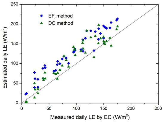
Figure 4.
Validations of daily ET estimations calculated by the DC method and temporal upscaled by the constant Efr method against with the original ET measurements.

Table 1.
Statistical items of daily ET estimations calculated by the DC method and temporal upscaled by the constant EFr method, validated with uncorrected and corrected EC measurements.
From the figure, it is obvious that both the DC and constant Efr methods generated overestimations of daily ET compared with the ET measurements, and the overestimation from the constant Efr method was greater. From the table, it can be seen that: (i) both the DC method and the constant Efr method resulted in overestimations of daily ET (positive MBE); (ii) the DC method performed better and generated more consistent ET estimations in terms of the original EC measurements, in which the MBE was 17.9 W/m2, the MAD was 20.9 W/m2, and the RMSE was 25.6 W/m2, respectively; (iii) the constant Efr method had larger estimation deviations, with an MBE of 32.8 W/m2, an MAD of 32.8 W/m2, and an RMSE of 35.7 W/m2; (iv) the constant Efr method had greater overestimation (with a higher averaged MBE) and daily Ets were overestimated on all the selected clear days (MAD = MBE), whereas some underestimations related to the DC method occurred on part of selected days (MAD > MBE); and (v) the constant Efr method had a larger R2 (0.926) than that of the DC method (0.879).
Therefore, both daily ET datasets estimated using the DC and constant Efr methods showed large deviations when compared with the EC measurements without correction of energy imbalance. To some extent, the overestimation of daily ET was partly assumed to come from the energy imbalance of the measured surface energy components on a diurnal day. Based on this assumption, it was expected that the estimated daily ET would result in better agreement with the EC measurements after correcting for the energy imbalance.
4.1.2. Evaluation with Flux Measurements after Correction
Figure 5a,b display the comparisons of daily ET estimations calculated with the DC method directly and temporal upscaled with the constant Efr method, with the EC measurements after correction of energy imbalance by the RE and BR schemes, respectively. The figures show that (i) daily ET estimations from both the DC and constant Efr methods were still overestimated when validated by the flux observations corrected with the RE scheme (Figure 5a), but overestimations were significantly decreased when compared to the evaluation results using the original flux measurement as validation; and (ii) both methods could effectively estimate daily ET when the energy imbalances were corrected by the BR scheme (Figure 5b); namely, the estimated daily Ets were more consistent with the flux measurements after correction of energy imbalance with the BR scheme than those corrected with the RE scheme.
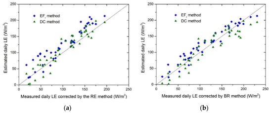
Figure 5.
Validations of daily ET estimations calculated by the DC method and temporal upscaled by the constant EFr method against with corrected EC flux measurements by (a) the RE scheme and (b) the BR scheme.
The statistical items of the daily ET validations are presented in Table 1. From the items in the table referring to the mean observed data, it can be seen that the average value of uncorrected daily ET measurements (94.9 W/m2) is much smaller than the corrected values, regardless if they were corrected with the BR (104.3 W/m2) or the RE (117.6 W/m2) schemes; thus, the undervalues of the daily ET measurements were further proved. Other statistical items related to the two estimation methods showed apparent differences when the estimation results were validated by corrected ET measurements using the RE and BR schemes.
When the EC measurements were corrected by the RE scheme, it was found that (i) both estimation methods still showed overestimations in daily ET estimations with positive MBE. In particular, the MBE from the DC and constant EFr methods was 7.4 and 19.8 W/m2, respectively; (ii) the DC method generated some underestimations of daily ET on a few selected days, as reflected by the larger difference between the MBE and MAD (7.4 and 16.1 W/m2, respectively); on the contrary, the constant EFr method still generated overestimations of daily ET on most selected days, shown by the small difference between the MBE and MAD (19.8 and 25.0 W/m2, respectively); (iii) both methods showed better results of daily ET estimation compared to that when validated using unclosed daily ET observations. A better performance of the DC method was noted, with the RMSE of 19.3 W/m2, compared to that of the constant EFr method with the RMSE of 29.7 W/m2; and (iv) both estimation methods showed similar R2 (0.893 and 0.898) in the linear regressions of the validations and estimations.
When the energy imbalance of daily ET measurements was corrected by the BR scheme, it was demonstrated that (i) daily ETs calculated through the DC method and upscaled with the constant EFr method both agreed best with the corrected ET measurements, with the lowest RMSEs of 18.2 and 16.2 W/m2, respectively; (ii) the DC method underestimated daily ET with a negative MBE (−4.7 W/m2), while the EFr method still had minimal overestimation of daily ET with positive MBE (10.5 W/m2); (iii) the similar value between the MBE and MAD (10.5 and 13.7 W/m2, respectively) of the constant EFr method further proved the overestimation on most selected days; and (iv) the constant EFr method had a larger R2 (0.940) than that of the DC method (0.890).
Overall, the DC method had similar or better performance compared to the constant EFr method for daily ET estimation when field data only were used as input, and the accuracies related to these two estimation methods varied slightly. Both methods tended to have serious overestimation compared to EC measurements, and the reason for this was that the energy imbalance caused some error in the surface energy components. When the energy imbalances were corrected, the overestimations were significantly reduced, particularly after correction by the BR scheme. Meanwhile, owing to its better performance, the BR correction scheme was applied to correct the energy imbalance in the following evaluations with the satellite data used as input.
4.2. Evaluation Based on Satellite Data
4.2.1. Estimation of Associated Parameters
Using the methods mentioned in Section 2.3, MODIS-based Ts, Rn, a, and G were retrieved and estimated. The estimations of these parameters based on MODIS data at satellite overpass times of 45 selected clear days were compared with ground-based measurements in our previous study [21]. MODIS-based Ts was compared with the temperature estimated from the measurements of upwelling and reflected downwelling longwave radiation because of the very limited spatial representativeness of the point-based Ts measurements. The bias (MODIS-based Ts minus ground-based Ts) and RMSE for the Ts estimation were 1.1 and 1.9 K, respectively, showing its high estimation accuracy. The bias and RMSE for the validation of the estimated Rn according to Equation (15) were 15.2 and 45.7 W/m2, respectively, showing good agreement with the ground-based measurements. The soil heat flux was calculated as a fraction of the surface net radiation, according to Equation (17), and then the surface available energy (surface net radiation minus soil heat flux) at the MODIS pixel scale was obtained and compared with ground measurements. The bias and RMSE for the validation of the estimated surface available energy were 4.4 and 37.6 W/m2, respectively, revealing a good agreement between the estimated and ground-measured values.
After the MODIS-based parameters were retrieved, the aerodynamic resistance (rae), decoupling coefficient (Ω) and surface resistance (rs) were then calculated. With the good performances of MODIS-based parameters guaranteeing confidence and reliability, together with the measurements of air humidity (ea) and air temperature (Ta) representing the atmospheric conditions, the instantaneous ET were estimated and daily ET were obtained by direct calculation with the DC method and by temporal upscaling with the constant EFr method.
4.2.2. Instantaneous ET Estimation with MODIS Data
The necessary parameter estimations were sufficient to provide accurate inputs for the calculation of instantaneous ET and decoupling coefficient Ω. The Ω result was also presented in our previous study, in which the DC method was developed [21]. Figure 6 shows the instantaneous ET over 45 MODIS/Terra overpass times estimated using MODIS data, compared with ET observations corrected by the BR scheme, which was validated to have excellent correction behavior in the above sections. Overall, the MODIS-based instantaneous ET was well calculated, with a small bias of 1.5 W/m2 and an average RMSE of 37.6 W/m2.
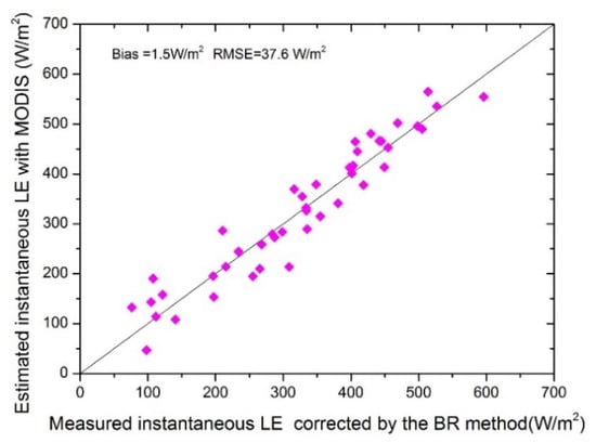
Figure 6.
Validation of instantaneous ET estimations based on MODIS data, with the ET measurements corrected by the BR scheme.
4.2.3. Evaluation of Daily ET Based on Remote Sensing Data
By accommodating the instantaneous ET and Ω based on satellite data collected on 45 selected clear days, the accuracies of daily ET calculated by the DC method and temporally upscaled by the constant EFr method were evaluated. During this evaluation process, the BR correction scheme was used to correct daily ET measurements to provide closed daily ET for validation. Scatter plots of daily ET estimations calculated directly by the DC method and by extrapolating the instantaneous ET through the EFr method vs. corrected daily ET measurements are shown in Figure 7, with statistical measures (MBE, MAD, RMSE, and R2) provided in Figure 8.
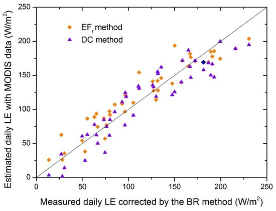
Figure 7.
Validations of daily ET estimations calculated directly by the DC method and temporal upscaled by the EFr method, based on MODIS data against with corrected ET measurements by the BR scheme.
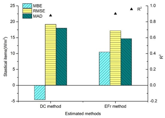
Figure 8.
Statistical items for daily ET estimations calculated directly by the DC method and temporal upscaled by the EFr method based on MODIS data against with corrected ET measurements by the BR scheme.
Comprehensive information from the scatter plots and statistical items suggests that both estimation methods can generate daily ET estimations with high accuracy based on satellite data. It could be seen that (i) the constant EFr method still overestimated daily ET and the related MBE, RMSE, and MAD were 5.6, 18.6, and 15.2 W/m2, respectively. The large difference between the MBE of 5.6 W/m2 and the MAD of 15.2 W/m2 revealed some underestimation of daily ET on a few selected days; (ii) daily ET was underestimated through the DC method, and the related MBE, RMSE, and MAD were −4.8, 22.5, and 19.0 W/m2, respectively. Similarly, the large difference between the MBE of −4.8 W/m2 and the MAD of 19.0 W/m2 also indicated some overestimation related to the DC method; (iii) the R2 from the constant EFr method was 0.901, a little larger than that from the DC method, 0.878. Overall, the DC method had similar MBE and RMSE compared to the EFr method, which is already widely applied in the extrapolation of instantaneous ET based on remote sensing data.
For better understanding the performances of these two estimation methods in daily ET calculation, Figure 9 shows the temporal variations in daily ET values calculated directly by the DC method and temporal upscaled by the EFr method against with ET measurements corrected by the BR scheme, during different winter wheat and summer corn growth stages. Overall, the temporal variations in daily ET from two methods have similar trends to that from ET measurements, and these variations vary considerably over the course of the season due to seasonally different radiations, atmospheric conditions, and growth stages of winter wheat and summer corn. Specifically, at winter wheat growth stage, daily ET estimations increased from a low value at the beginning to a high one in the summer of the next year and then decreased when the winter wheat was harvested; at the summer corn growth stage which was relatively shorter, daily ET also increased to a high value quickly and then decreased. The differences in daily ET variations may result from the different vegetation types which, in turn, lead to variations in the photosynthesis, water use, and fraction of incoming solar radiation and the interaction between air and surfaces.
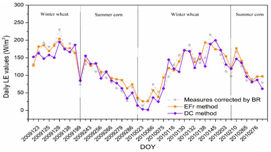
Figure 9.
Temporal variations in daily ET calculated directly by the DC method and temporal upscaled by the EFr method against with ET measurements corrected by the BR scheme, during different crop (winter wheat and summer corn) growth stages.
It is apparent that the accuracy of daily ET estimations based on satellite data was similar to that based on field data alone, compared with corrected daily ET measurements by the BR scheme, which further revealed the feasibility and effectiveness of both methods for daily ET estimations. A more serious overestimation from the EFr method was mainly due to the overestimation of instantaneous ET, which did not occur in using the DC method. In addition, the slight underperformance of these two estimation methods based on satellite data compared to that based on field data alone was also found, which was due to the daily ET estimation being also affected by the uncertainties from the parameter retrieval from remote sensing data, namely the uncertainties in Ts, Rn, and G estimations.
5. Discussion
In this study, we estimated daily ET using the DC and constant EFr methods and evaluated their performances. The DC method could calculate daily ET directly, while the constant EFr method is a widely used temporal upscaling method to obtain daily ET by extrapolating satellite-based instantaneous ET. It is well understood that daily ET estimations extrapolated by upscaling methods are co-determined by the interaction effect from the temporal upscaling method itself and the instantaneous ET calculation. Various accuracies for instantaneous ET calculations with different schemes in different applications have been reported [21,22,34,49,50]. The DC method has been proven to have the ability to directly calculate daily ET, in which instantaneous ET is not required, which may reduce some uncertainties. Therefore, through daily ET estimation and evaluation by direction calculation and temporal upscaling, this study provides a scientific basis for developing an operational and more accurate daily ET estimation method with easy access to data in future studies.
In order to separate the error caused by parameter retrievals from satellite data, at first, the DC calculation and EFr upscaling methods were applied to estimate daily ET using only the micrometeorological data recorded at the Yucheng site; then, MODIS data were used. It was found that the daily ET estimated through both methods based on remote sensing data was consistent with that based only on field data, and it was attributed to the high accuracy of the parameter inversion. The main deviations between the daily ET estimations and EC measurements in this study were mainly attributed to the serious energy imbalance of the EC energy components. It was expected that the performances of both two ET estimation methods would be improved after the corrections of the energy imbalance, and the performances based on remote sensing data would have similar features to those based only on field data as inputs. This conjecture was validated by the decreased errors in daily ET estimations when the results were compared with corrected EC measurements using the RE and BR schemes. In addition, daily Rn measurements, rather than daily available energy (Rn − G), were utilized in this study because the soil heat flux was generally assumed to be zero on a daily scale, which may be negligible in the application and can cause some estimated deviations. Other studies [26] have recommended that the average daily G should not be ignored, and whether the accuracy will be improved by considering the average daily G should be further tested. For the validation of the results, the primary source was usually considered to be from the scale mismatch between the ET data sets; namely, the spatial representativeness of the EC-derived ET is different with a MODIS pixel resolution of 1 km. In this study, the test area is topographically flat, the vegetation extends uniformly within the footprint area, and the footprints of the measured flux data are overall all within the MODIS pixel; therefore, the uncertainty caused by the footprint from the EC measurements is relatively small.
For these two estimation methods, the constant EFr method was shown to systematically overestimate the daily ET based on field data, regardless of whether the energy imbalances of the EC energy components were corrected. Overestimation of this upscaling method still occurred when it was used to extrapolate satellite-based instantaneous ET. In fact, a great number of other studies have reported overestimations of the constant EFr method [21,49]. The magnitude of overestimation decreased when the ET measurements were corrected, and the reduction tendency of the MAE and RMSE after the correction has also been observed in previous studies [21,50]. In this study, the DC method also overestimated daily ET compared to the observation data without correction or with correction by the RE scheme based on field data, whereas underestimation occurred when the energy imbalance was corrected by the BR scheme. Based on remote-sensing data, daily ET was also underestimated through this method, in accordance with the record in the study by Tang and Li [51], in which the detailed reason for the underestimation was presented. As for the comparison of these two estimation methods based on field data only, it appears that the DC method was more suitable for daily ET estimation when the RE scheme was used to correct the energy imbalance. Based on remote sensing data, the constant EFr method had a slightly higher accuracy. The estimation errors related to both estimation methods decreased when the energy imbalances were corrected; however, the degree of decrease was more significant in the DC method, indicating that the DC method was more sensitive to the energy imbalance.
We acknowledge some limitations of this study. Firstly, the test climate and landcover types were limited in Yucheng station and the time period was from late April 2009 to late October 2010, and further tests with more various climate types and geographic locations where there are long period meteorological materials are encouraged. Meanwhile, due to the similar input requirements and strong mechanisms of the DC method and the constant EFr method, only these two methods were compared in this study. In fact, there are other widely used temporal upscaling methods for daily ET estimations, such as the constant global solar radiation ratio method developed by Ryu et al. [21]. Van Niel et al. [50] used modeled global solar radiation and extraterrestrial solar radiation and observed global solar radiation and surface available energy as the upscaling proportions to test their performances in predicting daily ET and their findings suggested that using observed global solar radiation could perform best. However, the constant EFr method that can account for the variations in the meteorological elements in a diurnal cycle is not involved in their comparisons and therefore it needs to be further tested together with these upscaling methods in future studies.
Overall, the common advantage of the DC and constant EFr methods is that they both consider the variations in meteorological variables and are able to incorporate the effects of horizontal advection. Meanwhile, their common weakness lies in the requirements for detailed atmospheric variables as input, for example, air pressure, air temperature, global solar radiation, relative humidity, and wind speed in half-hourly or hourly time steps. Overall, when intensive meteorological measurements are readily available, the DC method is recommended for the direct estimation of daily ET to avoid errors from the estimation of instantaneous ET.
6. Conclusions
This study estimated daily ET using the DC method which can provide direct calculation of ET, and the constant EFr method which is a widely applied temporal upscaling method, using long-term field and satellite data covering the period from late April 2009 to late October 2010 at the Yucheng site in China. The results of both estimation methods were compared with those of closed and un-closed EC measurements. The findings of this study are expected to provide scientific guidance for the development and selection of a practical method with high accuracy for daily ET estimation.
With field data as input only, the constant EFr method overestimated daily ET by 10.5–32.8 W/m2 with RMSEs ranging from 16.2 to 35.8 W/m2; as for the DC method, the MBEs ranged from −4.7 to 17.9 W/m2, with the RMSEs of 15.0–20.9 W/m2. It is concluded that (i) the DC method outperformed the constant EFr method when the results were compared with those obtained using unclosed measurements, (ii) the DC method still performed better with reduced overestimation compared with corrected EC measurements by the RE scheme, and (iii) the constant EFr method outperformed the DC method after the ET measurements were corrected by the BR scheme. With satellite data as input, good agreement between the daily ET estimations and EC measurements showed that both the DC and constant EFr methods performed well. The constant EFr method slightly overestimated daily ET and the DC method underestimated daily ET, with MBE values of 5.6 and −4.8 W/m2, RMSE values of 18.6 and 22.5 W/m2, and MAD values of 15.2 and 19.0 W/m2, respectively.
Overall, the DC method exhibited similar or better performance than the well-known constant EFr method. Therefore, the DC method was proven to estimate daily ET directly and effectively. Our study provides a scientific basis for developing an operational and more accurate daily ET estimation method. When intensive meteorological measurements are readily available, the DC method is recommended for the direct estimation of daily ET to avoid errors from the estimation of instantaneous ET. Future study may focus on further application of the DC method in more various climate types and geographic locations with long time period meteorological materials and further comparison with other upscaling methods.
Author Contributions
Conceptualization, Y.J. and Y.W.; methodology, Y.J.; software, J.W.; validation, Y.J., J.W. and Y.W.; investigation, Y.J.; resources, Y.J.; data curation, J.W.; writing—original draft preparation, Y.J.; writing—review and editing, Y.J.; visualization, J.W.; supervision, Y.W.; funding acquisition, Y.J. All authors have read and agreed to the published version of the manuscript.
Funding
This research was funded by the Strategic Priority Research Program of the Chinese Academy of Sciences (Grant No. XDA28060400) and the National Natural Science Foundation of China (Grant No. 42001306).
Data Availability Statement
Not applicable.
Acknowledgments
We thank the Yucheng Comprehensive Site in China for providing the long-term meteorological and flux measurements and NASA for providing the MODIS serious products (https://earthdata.nasa.gov/) (accessed on 20 January 2018).
Conflicts of Interest
The authors declare no conflict of interest.
References
- Tanny, J. Microclimate and evapotranspiration of crops covered by agricultural screens: A review. Biosyst. Eng. 2013, 114, 26–43. [Google Scholar] [CrossRef]
- Jiang, S.; Wei, L.; Ren, L.; Xu, C.Y.; Zhong, F.; Wang, M.; Zhang, L.; Yuan, F.; Liu, Y. Utility of integrated IMERG precipitation and GLEAM potential evapotranspiration products for drought monitoring over mainland China. Atmos. Res. 2021, 247, 105141. [Google Scholar] [CrossRef]
- Granata, F. Evapotranspiration evaluation models based on machine learning algorithms—A comparative study. Agric. Water Manag. 2019, 217, 303–315. [Google Scholar] [CrossRef]
- Li, Z.L.; Tang, R.; Wan, Z.; Bi, Y.; Zhou, C.; Tang, B.; Yan, G.; Zhang, X. A review of current methodologies for regional evapotranspiration estimation from remotely sensed data. Sensors 2009, 9, 3801–3853. [Google Scholar] [CrossRef] [PubMed] [Green Version]
- Srivastava, A.; Sahoo, B.; Raghuwanshi, N. Evaluation of Variable Infiltration Capacity model and MODIS-Terra satellite-derived grid-scale evapotranspiration. J. Irrig. Drain Eng. 2017, 143, 1. [Google Scholar] [CrossRef] [Green Version]
- Bhattarai, N.; Wagle, P. Recent advances in remote sensing of evapotranspiration. Remote Sens. 2021, 13, 4260. [Google Scholar] [CrossRef]
- Chen, J.M.; Liu, J. Evolution of evapotranspiration models using thermal and shortwave remote sensing data. Remote Sens. Environ. 2020, 237, 111594. [Google Scholar] [CrossRef]
- Bastiaanssen, W.G.M.; Menent, M.; Feddes, R.A.; Holtslag, A.A.M. A remote sensing surface energy balance algorithm for land (SEBAL): 1. Formulation. J. Hydr. 1998, 212–213, 198–212. [Google Scholar] [CrossRef]
- Bastiaanssen, W.G.M.; Pelgrum, H.; Wang, J.; Ma, Y.; Moreno, J.F.; Roerink, G.J.; Van der, W.T. A Surface Energy Balance Algorithm for Land (SEBAL): Part 2 validation. J. Hydr. 1998, 212–213, 213–229. [Google Scholar] [CrossRef]
- Norman, J.M.; Kustas, W.P.; Humes, K.S. Source approach for estimating soil and vegetation energy fluxes in observations of directional radiometric surface temperature. Agric. Meteorol. 1995, 77, 263–293. [Google Scholar] [CrossRef]
- Mu, Q.Z.; Heinsch, F.A.; Zhao, M.S.; Running, S.W. Development of a global evapotranspiration algorithm based on MODIS and global meteorology data. Remote Sens. Enviro. 2007, 111, 510–526. [Google Scholar] [CrossRef]
- Farquhar, G.D.; von Caemmerer, S.; Berry, J.A. A biochemical model of photosynthetic CO2 assimilation in leaves of C 3 species. Planta 1980, 149, 78–90. [Google Scholar] [CrossRef] [Green Version]
- Tang, R.; Li, Z.L.; Tang, B. An application of the Ts–VI triangle method with enhanced edges determination for evapotranspiration estimation from modis data in arid and semi-arid regions: Implementation and validation. Remote Sens. Environ. 2010, 114, 540–551. [Google Scholar] [CrossRef]
- Tang, R.; Li, Z.L. An end-member-based two-source approach for estimating land surface evapotranspiration from remote sensing data. IEEE Trans. Geosci. Remote Sens. 2017, 55, 5818–5832. [Google Scholar] [CrossRef]
- Kumar, M.; Raghuwanshi, N.S.; Singh, R. Artificial neural networks approach in evapotranspiration modeling: A review. Irrig. Sci. 2011, 29, 11–25. [Google Scholar] [CrossRef]
- Issaka, A.I.; Paek, J.; Abdella, K.; Pollanen, M.; Huda, A.K.S.; Kaitibie, S.; Goktepe, I.; Haq, M.M.; Moustafa, A.T. Analysis and calibration of empirical relationships for estimating evapotranspiration in Qatar: Case study. J. Irrig. Drain Eng. 2017, 143, 05016013. [Google Scholar] [CrossRef]
- Kim, S.; Kim, H.S. Neural networks and genetic algorithm approach for nonlinear evaporation and evapotranspiration modeling. J. Hydr. 2008, 351, 299–317. [Google Scholar] [CrossRef]
- Srivastava, A.; Sahoo, B.; Raghuwanshi, N.S.; Chatterjee, C. Modelling the dynamics of evapotranspiration using Variable Infiltration Capacity model and regionally calibrated Hargreaves approach. Irrig. Sci. 2018, 36, 289–300. [Google Scholar] [CrossRef]
- Srivastava, A.; Kumari, N.; Maza, M. Hydrological response to agricultural land use heterogeneity using variable infiltration capacity model. Water Resour. Manag. 2020, 34, 3779–3794. [Google Scholar] [CrossRef]
- Kalma, J.D.; McVicar, T.R.; McCabe, M.F. Estimating land surface evaporation: A review of methods using remotely sensed surface temperature data. Surv. Geophys. 2008, 29, 421–469. [Google Scholar] [CrossRef]
- Ryu, Y.; Baldocchi, D.D.; Black, T.A.; Detto, M.; Law, B.E.; Leuning, R.; Miyata, A.; Reichstein, M.; Vargas, R.; Ammann, C.; et al. On the temporal upscaling of evapotranspiration from instantaneous remote sensing measurements to 8-day mean daily-sums. Agric. For. Meteorol. 2012, 152, 212–222. [Google Scholar] [CrossRef] [Green Version]
- Crago, R.D. Conservation and variability of the evaporative fraction during the daytime. J. Hydr. 1996, 180, 173–194. [Google Scholar] [CrossRef]
- Xu, T.; Liu, S.; Xu, L.; Chen, Y.; Jia, Z.; Xu, Z.; Nielson, J. Temporal upscaling and reconstruction of thermal remotely sensed instantaneous evapotranspiration. Remote Sens. 2015, 7, 3400–3425. [Google Scholar] [CrossRef] [Green Version]
- Delogu, E.; Olioso, A.; Alliès, A.; Demarty, J.; Boulet, G. Evaluation of multiple methods for the production of continuous Evapotranspiration estimates from TIR remote sensing. Remote Sens. 2021, 13, 1086. [Google Scholar] [CrossRef]
- Brutsaert, W.; Sugita, M. Application of self-preservation in the diurnal evolution of the surface energy budget to determine daily evaporation. J. Geophys. Res. Atmos. 1992, 97, 18377–18382. [Google Scholar] [CrossRef]
- Delogu, E.; Boulet, G.; Olioso, A.; Coudert, B.; Chirouze, J.; Ceschia, E.; Le Dantec, V.; Marloie, O.; Chehbouni, G.; Lagouarde, J.P. Reconstruction of temporal variations of evapotranspiration using instantaneous estimates at the time of satellite overpass. Hydrol Earth Syst. Sci. 2012, 16, 2995–3010. [Google Scholar] [CrossRef] [Green Version]
- Alfieri, J.G.; Anderson, M.C.; Kustas, W.P.; Cammalleri, C. Effect of the revisit interval and temporal upscaling methods on the accuracy of remotely sensed evapotranspiration estimates. Hydrol. Earth Syst. Sci. 2017, 21, 83–98. [Google Scholar] [CrossRef] [Green Version]
- Jiang, L.; Zhang, B.; Han, S.; Chen, H.; Wei, Z. Upscaling evapotranspiration from the instantaneous to the daily time scale: Assessing six methods including an optimized coefficient based on worldwide eddy covariance flux network. J. Hydr. 2021, 596, 126135. [Google Scholar] [CrossRef]
- Liu, Z. The accuracy of temporal upscaling of instantaneous evapotranspiration to daily values with seven upscaling methods. Hydrol. Earth Syst. Sci. 2021, 25, 4417–4433. [Google Scholar] [CrossRef]
- Tang, R.; Li, Z.L.; Sun, X. Temporal upscaling of instantaneous evapotranspiration: An intercomparison of four methods using eddy covariance measurements and MODIS data. Remote Sens. Environ. 2013, 138, 102–118. [Google Scholar] [CrossRef]
- Trezza, R. Evapotranspiration Using a Satellite-Based Surface Energy Balance with Standardized Ground Control. Ph.D. Thesis, Utah State University, Logan, UT, USA, 2002; p. 339. [Google Scholar]
- Allen, R.G.; Luis, S.; Pereira, D.R.; Martin, S. Crop Evapotranspiration-Guidelines for computing crop water requirements, FAO Technical Paper 56. FAO Rome 1998, 300, D05109. [Google Scholar]
- Almorox, J.; Grieser, J. Calibration of the Hargreaves–Samani method for the calculation of reference evapotranspiration in different Köppen climate classes. Hydrol. Res. 2016, 47, 521–531. [Google Scholar] [CrossRef] [Green Version]
- Colaizzi, P.D.; Evett, S.R.; Howell, T.A.; Tolk, J.A. Comparison of five models to scale daily evapotranspiration from one-time-of-day measurements. Trans. ASAE 2006, 49, 1409–1417. [Google Scholar] [CrossRef]
- Chávez, J.L.; Neale, C.M.U.; Prueger, J.H.; Kustas, W.P. Daily evapotranspiration estimates from extrapolating instantaneous airborne remote sensing et values. Irrig. Sci. 2008, 27, 67–81. [Google Scholar] [CrossRef]
- Kaya, Y.Z.; Zelenakova, M.; Üneş, F.; Demirci, M.; Hlavata, H.; Mesaros, P. Estimation of daily evapotranspiration in Košice City (Slovakia) using several soft computing techniques. Theor. Appl. Climatol. 2021, 144, 287–298. [Google Scholar] [CrossRef]
- Fan, J.; Yue, W.; Wu, L.; Zhang, F.; Cai, H.; Wang, X.; Lu, X.; Xiang, Y. Evaluation of SVM, ELM and four tree-based ensemble models for predicting daily reference evapotranspiration using limited meteorological data in different climates of China. Agric. For. Meteorol. 2018, 263, 225–241. [Google Scholar] [CrossRef]
- Jiang, Y.; Jiang, X.; Tang, R.; Li, Z.L.; Zhang, Y.; Huang, C.; Ru, C. Estimation of daily evapotranspiration using instantaneous decoupling coefficient from the MODIS and field data. IEEE J. Sel. Top. Appl. Earth Obs. Remote Sens. 2018, 11, 1832–1838. [Google Scholar] [CrossRef]
- McNaughton, K.G.; Jarvis, P.G. Predicting effects of vegetation changes on transpiration and evaporation. In Water Deficits and Plant Growth; Kozlowski, T.T., Ed.; Academic Press: Cambridge, MA, USA, 1983; Volume VII, pp. 1–47. [Google Scholar]
- Boegh, E.; Soegaard, H.; Hanan, N.; Kabat, P.; Lesch, L. A remote-sensing based study of the NDVI–Ts relationship and transpiration from sparse vegetation in the Sahel based on high-resolution satellite data. Remote Sens. Environ. 1999, 69, 224–240. [Google Scholar] [CrossRef]
- Allen, R.G.; Walter, I.A.; Elliott, R.; Howell, T.A.; Itenfisu, D.; Jensen, M.E. The ASCE Atandardized Reference Evapotranspiration Equation. American Society of Civil Engineers. 2005. Available online: https://epic.awi.de/id/eprint/42362/1/ascestzdetmain2005.pdf (accessed on 20 January 2018).
- Boegh, E.; Soegaard, H.; Thomsen, A. Evaluating evapotranspiration rates and surface conditions using Landsat TM to estimate atmospheric resistance and surface resistance. Remote Sens. Environ. 2002, 79, 329–343. [Google Scholar] [CrossRef]
- Tang, B.; Li, Z.L. Estimation of instantaneous net surface longwave radiation from MODIS cloud-free data. Remote Sens. Environ. 2008, 112, 3482–3492. [Google Scholar] [CrossRef]
- Tasumi, M.; Allen, R.G.; Trezza, R. At-surface reflectance and albedo from satellite for operational calculation of land surface energy balance. J. Hydrol. Eng. 2008, 13, 51–63. [Google Scholar] [CrossRef]
- Mauder, M.; Foken, T. Documentation and Instruction Manual of the Eddy-Covariance Software Package TK3 (Update). UNIVERSITÄT BAYREUTH Abt. Mikrometeorologie. 2015. Available online: https://epub.uni-bayreuth.de/2130/1/ARBERG062.pdf (accessed on 20 January 2018).
- Foken, T. The energy balance closure problem: An overview. Ecol. Appl. 2008, 18, 1351–1367. [Google Scholar] [CrossRef]
- Anderson, M.C.; Norman, J.M.; Diak, G.R.; Kustas, W.P.; Mecikalski, J.R. A two-source time-integrated model for estimating surface fluxes using thermal infrared remote sensing. Remote Sens. Environ. 1997, 60, 195–216. [Google Scholar] [CrossRef]
- Jiang, Y.; Tang, R.; Jiang, X.; Li, Z.L. Impact of clouds on the estimation of daily evapotranspiration from MODIS-derived instantaneous evapotranspiration using the constant global shortwave radiation ratio method. Int. J. Remote Sens. 2019, 40, 1930–1944. [Google Scholar] [CrossRef]
- Gentine, P.; Entekhabi, D.; Chehbouni, A.; Boulet, G.; Duchemin, B. Analysis of evaporative fraction diurnal behaviour. Agric. For. Meteorol. 2007, 143, 13–29. [Google Scholar] [CrossRef] [Green Version]
- Niel, T.G.V.; Mcvicar, T.R.; Roderick, M.L.; Dijk, A.I.J.M.V.; Renzullo, L.J.; Gorsel, E.V. Correcting for systematic error in satellite-derived latent heat flux due to assumptions in temporal scaling: Assessment from flux tower observations. J. Hydrol. 2011, 409, 140–148. [Google Scholar] [CrossRef]
- Tang, R.; Li, Z.L. An improved constant evaporative fraction method for estimating daily evapotranspiration from remotely sensed instantaneous observations. Geophys. Res. Lett. 2017, 44, 2319–2326. [Google Scholar] [CrossRef]
Publisher’s Note: MDPI stays neutral with regard to jurisdictional claims in published maps and institutional affiliations. |
© 2022 by the authors. Licensee MDPI, Basel, Switzerland. This article is an open access article distributed under the terms and conditions of the Creative Commons Attribution (CC BY) license (https://creativecommons.org/licenses/by/4.0/).