Abstract
Synthetic aperture radar (SAR) can detect ground information with high precision, which provides another opportunity for the retrieval of rain. Rainfall intensities in East Asia are mainly moderate. The current retrieval algorithms have high accuracy in rainstorms, but they overestimate the rainfall intensity greatly in moderate rain. Therefore, it is very important to reduce the retrieval error of SAR in moderate rain. After analyzing the scattering model of precipitation, this paper proposes an algorithm for retrieving 2-D moderate rain distribution (MRA). Since the 2-D distribution of rain is related to the vertical and horizontal distributions, MRA combines the empirical regression equation with the directional model of rain rates at different levels to retrieve the vertical distribution of precipitation. Compared with the model-oriented statistical (MOS) algorithm, MRA reduces the root mean square error when retrieving the surface rain rate from 2.6 to 0.1. In addition, based on the high-precision rain parameters retrieved by MRA, the horizontal distribution is retrieved through the likelihood distance. This horizontal distribution retrieval method not only has less amount of calculation but also avoids the difficulties of mathematical analysis.
1. Introduction
Precipitation is a key component of the global thermal cycle and drives the atmosphere and surface water cycle [1,2,3]. The accurate measurement of precipitation can provide scientific guidance for the geochemical cycle, industrial and agricultural production, and freshwater supply. Precipitation varies greatly in different regions [4]. In East Asia, the average value of the annual ground rain rate ranges from 1.7 mm/h to 10.2 mm/h [5]. Even in areas with high precipitation, such as Sanya, the time probability of rain rate above 21.9 mm/h is only 0.01 [6], and the common rain rates are between 1 mm/h and 15 mm/h. Therefore, it is very important to consider the distribution of moderate rain (surface rain rates between 1 mm/h and 15 mm/h).
At present, the precipitation observation system constructed by meteorological radars and extensive rain gauge networks can accurately estimate rain in conventional terrain, but it cannot accurately estimate high variability differential precipitation in complex terrain [7]. As a high-altitude detection technology, satellite remote sensing can effectively avoid the defects of rain gauges and ground-based weather radars limited by geographical location, and provide a larger spatial range of precipitation distribution information. Satellite remote sensing measures precipitation in two ways: passive and active. Passive remote sensing mainly refers to spaceborne visible infrared radiometer and spaceborne microwave radiometer, while active remote sensing mainly refers to spaceborne precipitation radar, such as precipitation radar (PR) and dual-frequency precipitation radar (DPR) [8]. The emergence of spaceborne PR measurement largely offset the tropical and marine area precipitation data, but it may ignore or underestimate the precipitation intensity for significant shallow precipitation [9]. At the same time, due to the high costs and the difficult procurement of components, only a few countries have on-orbit spaceborne precipitation radar.
Synthetic aperture radar (SAR) is an active microwave remote sensing technology, which can obtain surface information stably and continuously with high resolution at all times [10,11]. With the development of SAR technology, these high-resolution ground data are gradually applied in various fields, such as the detection of water areas, management of watersheds, supplementation of optical images, object detection, and identification of terrain [12,13,14,15]. Since 1988, China has started research on spaceborne SAR and has launched more than 10 spaceborne SAR satellites of various types. The working frequency bands cover L, S, C, and X, ranging from low-resolution discovery and identification to high-resolution targets [16,17]. For example, the X-band HY-2 satellite, the S-band HJ-1C satellite, and the C-band GF-3 03 satellite were launched in 2011, 2012, and 2022, respectively [18,19,20]. X-band (10 GHz) is very close to Ku-band (14 GHz) and is also sensitive to precipitation. Many scholars have shown that X-band SAR (X-SAR) can detect the distribution of surface precipitation with a horizontal distance of less than 100 m [21,22]. At the same time, X-SAR can not only reduce the errors caused by cirrus clouds in precipitation retrieval [23], but its combination with data of microwave radiation can also solve the problems caused by uneven beam congestion [24]. Therefore, the precipitation retrieval using X-SAR echo data can supplement the precipitation radar and improve the current problems of the small number of precipitation satellites in orbit and the uneven distribution of global precipitation retrieval.
In 1991, Pichugin et al. set up a rainfall model assuming that the vertical distribution is homogeneous and solved the rainfall attenuation expression through the Volterra integral equation (VIE) of the second kind [25]. However, when this method is applied to vertical inhomogeneous models, the computational complexity of the analytical solution increases significantly. In 2006, Weinman et al. established a model-oriented statistical (MOS) algorithm, which solved the rain rate by analyzing the contour lines in the contoured frequency by altitude diagrams (CFAD) [26,27]. MOS has a good effect on rainstorms, but it is poor in moderate rain and requires a large number of empirical parameters. At the same time, MOS needs to construct a suitable simulation database for retrieving the horizontal distribution, which makes the calculation redundant. In 2016, Xie et al. proposed the model-oriented statistical and Volterra integration (MOSVI) algorithm [28]. It uses a mathematically analytic method to reduce the amount of calculation when retrieving the horizontal distribution in a single-layer precipitation model, but it is difficult to solve the analytical solution in multi-layer precipitation models. Furthermore, MOSVI will still overestimate the rain rate in moderate rain.
Combined with the above analysis, this paper proposes MRA, an algorithm for retrieving the 2-D distribution of moderate rain. MRA aims to reduce the overestimation error when retrieving moderate rain rate and avoid the problem of the complex calculation when retrieving the horizontal distribution. In terms of retrieving the vertical distribution, MRA proposes an empirical regression equation between the surface rain rate and the radar cross-section of the precipitation area to retrieve the surface rain rate. The relative error of the retrieval surface rain rate obtained by the equation is between 0.1 and 0.28. Compared with MOS, MRA reduces the root mean square error from 2.6 to 0.1. At the same time, MRA also combines the empirical regression equation with the direct model of rain rates at different levels to retrieve the vertical distribution of precipitation. In terms of retrieving horizontal distribution, MRA proposes a mathematical-statistical method based on the idea of maximum likelihood classification. This method not only avoids the complex problem in VIE but also solves the problem of computational redundancy in MOS. Compared with MOS, MRA reduces the calculation amount of retrieving precipitation horizontal distribution by 97%. Finally, the high-precision two-dimensional distribution of precipitation in moderate rain is obtained by combining the horizontal distribution and vertical distribution.
2. Normalized Radar Cross Section of Precipitation
Attenuation occurs when microwave energy travels along the propagation path in the precipitation area. This is because when microwaves are projected onto precipitation particles, part of the energy is scattered, and another part of the energy is absorbed, thereby weakening the microwaves. The scattering characteristics of precipitation particles are the basis for the measurement of precipitation by radar. Scattering is mainly represented by the radar cross section (RCS). In 1994, a large number of SAR images in X, C, and I bands were acquired from the Space Shuttle “Endeavour”. It is found that, on the X-band images, the precipitation area can be distinguished [29]. This is because the RCS of the precipitation area is lower than the RCS of the rainless area. The size, distribution, and dielectric constant of the precipitation particles will cause the RCS to change [30]. Since freezing makes highly polar molecules in liquid water bound in the crystalline lattice, the dielectric constant of snow is much lower than that of rain. The effects of rain and snow on the RCS are also different [31]. Considering both snow particles and rain particles in this paper, the two-layer precipitation model (ignoring the melt layer) is shown in Figure 1.
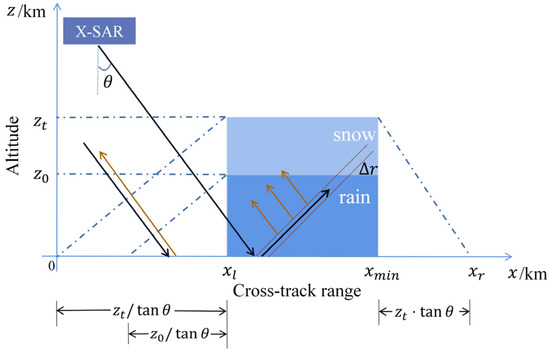
Figure 1.
The cross-section of the two-layer precipitation model.
In this model, x is the cross-track coordinate, z is the height coordinate, zt is the top height of the snow layer, z0 is the top height of the rain layer and is the slant off-nadir angle of X-SAR. is the starting point of the precipitation area, is the ending point of the precipitation area, and is the farthest cross-track distance affected by the precipitation area. Microwave pulses emitted by X-SAR are approximated as plane wavefront slices, shown as a pair of lines with a width of in Figure 1. The error caused by this approximation is about 0.2 km [27], which is within the acceptable range.
According to the cross-section model of precipitation, the normalized radar cross section (NRCS) of precipitation area can be obtained [32], which will be denoted as in this paper. of the precipitation area is the sum of the surface scattering cross-section and the volume scattering cross section :
where , , , and are the upper and lower limits of the integration of the path projection of the radar beam in the precipitation area onto the z-axis. The and are the upper and lower limits of the integration of the path projection of the reflected microwaves via the ground in the precipitation area onto the z-axis. is the RCS of no rain area. Concerning the typical value of the average RCS of vertically polarized radiation incident on land at 30°, is about −7 dB [33]. is the attenuation coefficient and is the coefficient of radar volume scattering, both of which can be obtained according to Equation (4) [26] and Equation (5) [27]:
where is an expression of a negative refractive index with a value of 0.93 for rain and a value of 0.19 for snow [26,27]. is the wavelength of the radar incident microwave, which is about 3.1 cm for X-SAR. For rain, the empirical values of a, b, c, and d are 2.6 × 10⁻³, 1.11, 300, and 1.85; for snow, the empirical values of a, b, c, and d are , 1.6, 182, and 1.6 [34].
As the incident microwave moves along the cross-track in the range of , will increase above due to the existence of the of snow particles. As the microwave moves in the range of , the of rain particles is enhanced and still increases. However, because the of rain particles is less than snow particles, the growth rate of in this phase decreases compared to the previous phase. As the microwave moves in the range of , the is greatly reduced by the attenuation of the precipitation area in the bidirectional path of the microwave transmission. Although the of snow and rain particles is enhancing, the increase is small. So, the continues to decrease to its lowest point, that is the . When the microwave moves out of the precipitation area in the range of , the attenuation decreases and the starts to increase until it returns to . The simulation of NRCS is shown in Figure 2.
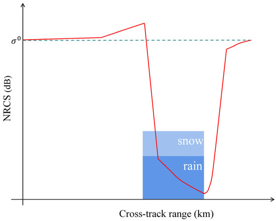
Figure 2.
The NRCS simulation result.
3. Retrieval of Vertical Distribution
It is assumed that the two-dimensional precipitation distribution can be divided into vertical distribution and horizontal distribution , and the two are uncorrelated and can be retrieved separately.
There are 18 existing , and the three most commonly used: rectangular distribution, triangular distribution and trapezoidal distribution will be used in this paper.
3.1. Retrieval of by MOS Algorithm
The retrieval of vertical distribution in MOS requires the help of CFAD. Through the approximation of contour lines, the rain rates can be obtained [35]:
where is the freezing coefficient. A larger indicates heavier snow, 1.13, 21.62, 2.58, and 23.3 are empirical values, which are calculated under = 30°, = 13 km and z0 = 4.5 km. is the width of the precipitation area. For horizontal distributions of the rectangle, triangle and trapezoid, can be retrieved by the following equations [27,28]:
From Equations (8) and (9), it is found that the rain rates of the rain layer and snow layer depend on the surface rain rate , so the retrieval accuracy of largely determines the retrieval accuracy of .
For ease of reading, variables designated with circumflexes are used below to denote the values retrieved from the algorithm, and variables without circumflexes to denote the real or given values. For example, represents the given surface rain rate, and represents the surface rain rate retrieved by the algorithm. Weinman et al. evaluated the error of of MOS in rainstorms and torrential rains. For the 18 sets of data with surface rain rates ranging from 15 mm/h to 160 mm/h, the root mean square error between and is evaluated by Equation (13) and is 0.1 [26]. From the experimental results, the retrieval accuracy of MOS was higher in rainstorms.
where m represents the number of data sets.
However, a rainstorm of more than 15 mm/h is not always the case, so this paper tests the retrieval results of MOS in moderate rain. For simulated NRCS data with surface rain rates ranging from 1 mm/h to 15 mm/h, retrieved by MOS are shown in Figure 3. The horizontal distribution of precipitation used in the following section is a rectangle unless otherwise noted. Figure 3 shows is overestimated with an of about 2.6. Therefore, the retrieval error of MOS is large in the case of moderate rain.
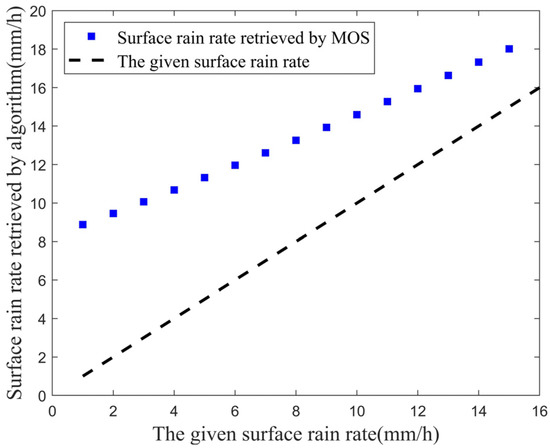
Figure 3.
Retrieved surface rain rates by MOS and the given rain rates.
3.2. Retrieval of by MRA Algorithm
To reduce the retrieval error of and simplify the retrieval equation, MRA proposed an empirical regression equation between and . The equation is mainly based on the fitting relationship between NRCS and surface rain distribution [36]:
where and are empirical values,
Equation (14) is obtained by fitting TerraSAR-X (TSX) and next-generation weather radar (NEXRAD) data at the same time and in the same place. Take the surface rain distribution retrieved from data of NEXRAD as the true value. By combining the relationship between radar reflectivity factor and in NEXRAD and the relationship between NRCS and in TSX, it is obtained that the power-law relationship of the NRCS measured by TSX and the true value as shown in Equation (14). Using a large number of TSX data in moderate rain for fitting, is 2.84 and is 1.83.
Equation (14) is obtained by fitting the data, but it can also be derived theoretically. By simulating the NRCS in moderate rain, the relationships between , , and in different surface rain rates are shown in Figure 4. Figure 4a–c show NRCS, and , respectively, when the surface rainfall rate is 15 mm/h. It is clearly shown in Figure 4c that is smaller than by more than one order of magnitude in the precipitation of 15 mm/h. Furthermore, the proportion of decreases as decreases as shown in Figure 4e. Therefore, can be neglected relative to in moderate rain, and then in Equation (1) can be expressed as:
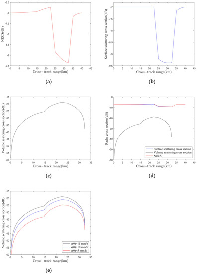
Figure 4.
Simulation of NRCS in moderate rain. (a) The normalized radar cross section of mm/h; (b) the surface scattering cross section of mm/h; (c) the volume scattering cross section of mm/h; (d) components of normalized radar cross section of mm/h and (e) comparison of the volume scattering cross section of mm/h, 10 mm/h, and 5 mm/h.
can be expressed by effective path-integrated rain rate [36]:
where is the scale factor and is the horizontal distribution shape exponent.
The integral of can be obtained by combining Equations (4) and (17):
Bring Equation (18) into Equation (16):
After taking the logarithm and changing the base on both sides simultaneously, can be written as:
This form is the same as Equation (14), so it is proved from both theoretical derivation and data fitting that surface rain distribution can be expressed in the exponential form of .
It is assumed that consists of a horizontal distribution and a surface rain rate :
In Appendix A, a simple test of the effect of Equation (14) on retrieving is performed. The test results show that Equation (14) has a small error in retrieving the surface rain rate, but a large error in retrieving the horizontal distribution. To reduce the error introduced by the empirical regression equation in retrieving the horizontal distribution, only is retained as the retrieval result.
MRA uses Equation (22) to retrieve the surface rain rate in moderate rain. Substituting into Equations (8) and (9) to obtain the rain rate of different heights. Then the horizontal distribution algorithm in Section 4 is used to invert , and the two-dimensional distribution of moderate rain can be output. The process of MRA is shown in Figure 5. The retrieval methods of , and are described in Appendix B.
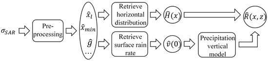
Figure 5.
The process of MRA.
4. Retrieval of Horizontal Distribution
The three most commonly used horizontal distributions can be shown as:
When and , it represents rectangular and triangular horizontal distributions, respectively. When , it represents trapezoidal horizontal distribution.
The central idea of the retrieval horizontal distribution is to use the idea of maximum likelihood classification to find a set of simulated data that are most similar to the data to be retrieved. The specific approach is to measure some simulation data with known horizontal distributions and the data to be retrieved one by one and calculate the likelihood distance between the two sets of data. The used in the set of simulation data with the smallest likelihood distance is the . Equations (24)–(27) extract the distribution characteristics of each set of data in terms of four aspects: mean , variance , skewness , and kurtosis . There are positive and negative in a set of data. By calculating the positive and negative separately, eight statistical parameters can be obtained.
where is the amount of a set of data.
In addition to the above 8 statistical values, it is also necessary to focus on the gradient near the precipitation starting point. In this paper, the gradient values at , km, and km are examined. Together with the first 8 statistical values, a set of data yields 11 measurements, which can form an 11-dimensional statistical vector.
The statistical vector of a set of simulation data is denoted as , and the statistical vector of the data to be retrieved is denoted as . The likelihood distance of the two sets of data can be expressed as:
where is the covariance matrix with a dimension of 11 × 11.
As is not only affected by the difference between the horizontal distributions of the two sets of data but also affected by the difference in other parameters such as . Therefore, the simulation data should keep parameters except for as consistent as possible with the data to be retrieved. Through the retrieval process of MRA, it is found that , , and other parameters can be obtained with high accuracy before the retrieval of . Using these parameters, can be calculated according to Equations (8) and (9). Assuming a kind of , a simulated rain distribution can be obtained. As can be seen from Section 2, a set of can be obtained according to Equations (2) and (3) when the is known. The likelihood distance calculated by and the data to be retrieved only represents the difference between the simulated horizontal distribution and the real horizontal distribution. In the case of considering only the three common horizontal distributions, it is necessary to construct only 3 sets of simulation data and calculate 44 statistics.
In MOS, retrieving the horizontal distribution of rain requires 50 sets of simulation NRCS, and a total of about 1650 statistical values need to be calculated. Compared with MOS, if only three horizontal distributions are considered, this method only needs three sets of simulation data, and the amount of calculation is greatly reduced. Compared with the inversion method of VIE, this method avoids the solving steps of analytical solution and is simpler and more intuitive.
5. Simulation and Discussion
In this section, the MRA will be simulated to retrieve the surface rain rate, horizontal distribution and two-dimensional distribution of precipitation. For X-SAR with a slant off-nadir angle of 30°, set km, km and . Considering the resolution of SAR and the cross-track distance affected by precipitation, each set of NRCS data consists of 200 data points. Parameters with different values in different sets of data, such as , and , will be described in detail before each simulation.
5.1. Simulation of Surface Rain Rate
In cases 1–3, the surface rain rates of rectangular, triangular, and trapezoidal rain clouds were retrieved using MRA, respectively. Fifteen sets of NRCS data were used in each case. The parameters for the 15 sets of data are: km and surface rain rates between 1 mm/h and 15 mm/h. The relative error (RE) is defined as Equation (29):
Case 1: Assume that the horizontal distribution of all NRCS data is a rectangle and the retrieval results are shown in Figure 6. The RE of MRA ranges from 0.01 to 0.28 and the RE of MOS ranges from 0.23 to 8.32.
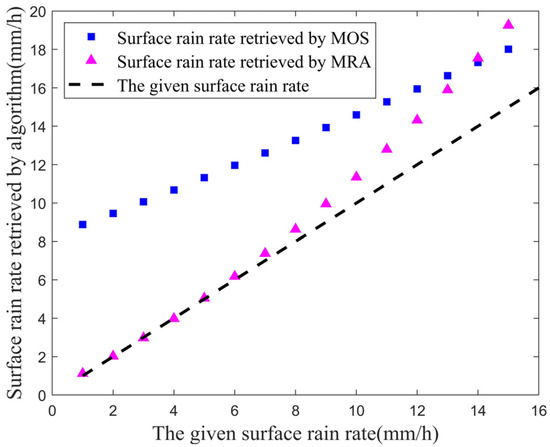
Figure 6.
Surface rain rates retrieved by MRA and MOS under rectangular horizontal distribution.
Case 2: Assume that the horizontal distribution of all NRCS data is the triangle and the retrieval results are shown in Figure 7. The RE of MRA ranges from 0.03 to 0.19 and the RE of MOS ranges from 0.32 to 8.44.
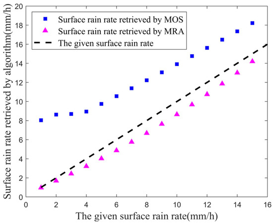
Figure 7.
Surface rain rates retrieved by MRA and MOS under triangular horizontal distribution.
Case 3: Assume that the horizontal distribution of all NRCS data is trapezoid and the retrieval results are shown in Figure 8. The RE of MRA ranges from 0.02 to 0.17 and the RE of MOS ranges from 0.29 to 9.76.
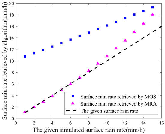
Figure 8.
Surface rain rates retrieved by MRA and MOS under trapezoidal horizontal distribution.
Overall, the RE of MRA is much smaller than MOS in moderate rain. Figure 6, Figure 7 and Figure 8 show the error of MRA increases with the increase of , which is due to the increase of of rain particles when the rain is heavier. At this time, the error caused by ignoring in Equation (22) increases.
Table 1 shows the root mean square error of MRA and MOS in cases 1–3. The of MRA under the rain of three horizontal distributions are very close to each other, all around 0.15, but the of MOS is around 2.6. The experiment proves that MRA can effectively reduce the retrieval error of the surface rain rate in moderate rain.

Table 1.
Root mean square error of MRA and MOS.
5.2. Simulation of Horizontal Distribution
There are four sets of data to be retrieved to verify the effectiveness of this method in cases 4–7. of the four sets of data is 15 mm/h. The values of parameters such as horizontal distribution in each set of data are shown in Table 2.
Table 2.
The horizontal distribution of data to be retrieved in cases 4–7.
In each case, it is necessary to construct three sets of simulation data with different horizontal distributions. The horizontal distributions used by the three sets of simulation data are rectangle (), triangle () and trapezoid (), where represents the rain width obtained from the data to be retrieved in each case. Then calculate the likelihood distance between simulation data and data to be retrieved. The used in the set of simulation data with the minimum likelihood distance is selected as . Table 3 shows the and the retrieval of horizontal distribution in cases 4–7.
Table 3.
Likelihood distance between simulation data and data to be retrieved.
The correct retrieval results of the were obtained for three horizontal distributions of the retrieved data as shown in Table 3.
5.3. Simulation of 2-D Distribution of Moderate Rain
The retrieval effect of MRA on the two-dimensional distribution of moderate rain is shown in cases 8–10. The parameters of the data used in the three cases are: mm/h, and km.
Case 8: Set the rain type as rectangular distribution ( km). The given two-dimensional distribution of rain, the two-dimensional distribution of rain retrieved by MRA and the absolute error diagram are shown in Figure 9. The surface rain rate retrieved by MRA is 4.9 mm/h and the relative error is 0.02.
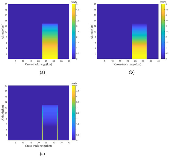
Figure 9.
Two-dimensional distribution of rectangular rain. (a) The given two-dimensional distribution of rain; (b) the two-dimensional distribution of rain retrieved by MRA; and (c) the absolute error diagram.
Case 9: Set the rain type as triangular distribution ( km). The given two-dimensional distribution of rain, the two-dimensional distribution of rain retrieved by MRA and the absolute error diagram are shown in Figure 10. The surface rain rate retrieved by MRA is 4.3 mm/h and the relative error is 0.14.
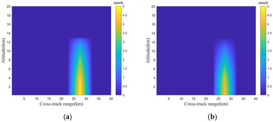
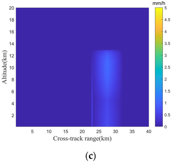
Figure 10.
Two-dimensional distribution of triangular rain. (a) The given two-dimensional distribution of rain; (b) the two-dimensional distribution of rain retrieved by MRA; and (c) the absolute error diagram.
Case 10: Set the rain type as trapezoidal ( km). The given two-dimensional rainfall distribution, the two-dimensional rainfall distribution retrieved by MRA and the absolute error diagram are shown in Figure 11. The surface rain rate retrieved by MRA is 4.8 mm/h and the relative error is 0.04.
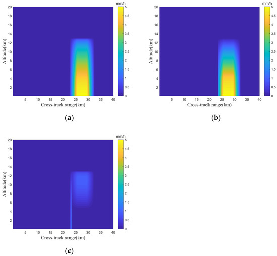
Figure 11.
Two-dimensional distribution of trapezoidal rain. (a) The given two-dimensional distribution of rain; (b) the two-dimensional distribution of rain retrieved by MRA; and (c) the absolute error diagram.
Figure 9c, Figure 10c and Figure 11c show that the absolute error between the retrieved two-dimensional distribution of moderate rain and the given two-dimensional distribution of rain is very small, especially in the rainfall layer. The locations with larger absolute errors occur at the edges of the precipitation area, especially in the rain of rectangular distribution as shown in Figure 9c. This is caused by the error of retrieving precipitation width. The relative error of retrieval width is about 0.03 in cases 8–10, which is within an acceptable range.
At different heights, the height at which the absolute error suddenly increases is the junction height of the snowfall layer and the rainfall layer. This is due to the overestimation phenomenon in the retrieval of the freezing coefficient . The accurate retrieval of is also a direction for subsequent research.
6. Conclusions
This paper introduces a two-layer model for X-SAR precipitation measurement and simulates the NRCS of precipitation. After analyzing the proportional relationship between the components of NRCS, the MRA is proposed to improve the retrieval accuracy in moderate rain. MRA can effectively retrieve the vertical distribution together with the horizontal distribution and output the two-dimensional distribution of moderate rain. The retrieval effect of MRA in moderate rain is verified using simulated echo data under different horizontal distributions. The results show that the root mean square error of MRA is around 0.15. Compared with MOS, MRA reduces the root mean square error in moderate rain by 96%. In addition, MRA also uses mathematical statistics to retrieve the horizontal distribution. The method of mathematical statistics avoids the difficulty of solving analytical solutions in VIE and computational redundancy in MOS.
Obviously, through the above analysis, MRA can be used for daily precipitation detection. At the same time, MRA also has certain utility in preventing natural disasters with precipitation changes as the main driving factor, such as drought and mudslides. The occurrence of drought is due to the fact that the water expenditure of the region is much greater than the water income in a certain period of time. For traditional droughts, MRA can measure precipitation with high accuracy, which can be combined with evapotranspiration data to contribute to drought prevention. For mudslides, the latest research has proved that the prone areas of mudslides can be predicted through the annual precipitation [37]. MRA can provide a reliable estimate of annual precipitation through long-term observations of remote sensing satellites, thereby preventing mudslides. In addition to annual precipitation, estimates of individual precipitation may also be useful in analyzing mudslides. For example, in Indian Himalayas, a mudslide caused by avalanches and rock avalanches occurred. The rapid flow of the mudslide has resulted in huge human casualties and loss of property [38]. In addition to the melting of glaciers separated in the avalanche, which increases the velocity of the mudslide, the precipitation which occurs before the avalanche is also a cause of the rapid movement of the mudslide. MRA can roughly determine the proportion of precipitation in the mudslide by accurately estimating the amount of precipitation, so as to further determine the proportion of the separated glacier meltwater in the mudslide. This could contribute to the study of how avalanches affect mudslides.
The focus of this paper is on the retrieval algorithm, so some parameters are simplified. For example, the influence of rainfall on the RCS of the sea surface is ignored, and this is also the direction that should be worked on in the future. Moreover, the vertical distributions of rain in different regions and types also deserve further study.
Author Contributions
Conceptualization, Y.X. and R.W.; methodology, S.L.; software, S.L.; validation, S.L., T.L., X.Y. and Z.X.; formal analysis, S.L.; writing—original draft preparation, S.L.; writing—review and editing, S.L., T.L. and X.Y. All authors have read and agreed to the published version of the manuscript.
Funding
This research was funded by the National Natural Science Foundation of China, grant number 62071286.
Institutional Review Board Statement
Not applicable.
Informed Consent Statement
Not applicable.
Data Availability Statement
Not applicable.
Conflicts of Interest
The authors declare no conflict of interest. The funders had no role in the design of the study; in the collection, analyses, or interpretation of data; in the writing of the manuscript, or in the decision to publish the results.
Appendix A
This appendix is the simulation of Equation (14) to test the performance of Equation (14) in retrieving surface rain distribution. The simulation results are very important to the proposal of Equation (22).
For X-SAR with a slant off-nadir angle of 30°, set km, km. According to Equations (1)–(3), three sets of NRCS data can be constructed and used in cases A1–A3, respectively. The same parameters of the three sets of data are km and . Among the three sets of data, the different parameters are and , which are listed in the second and third columns of Table A1. Each set of NRCS data consists of 200 data points.
The retrieval results in each case are shown in columns 4 and 5 of Table A1. represents the maximum surface rain rate retrieved by Equation (14). represents the relative error between and .
Table A1.
The attributes of NRCS data and retrieval results.
Table A1.
The attributes of NRCS data and retrieval results.
| case A1 | 5 | rectangle | 5.1 | 0.02 |
| case A2 | 10 | trapezoid | 10.8 | 0.08 |
| case A3 | 15 | triangle | 14.1 | 0.06 |
From Table A1, can be calculated and is 0.05. Compared with the retrieval root mean square error of MOS in moderate rain, the retrieval error of the empirical regression equation is much smaller.
The given surface rain distribution and the retrieval results are shown in Figure A1. The corresponding ordinate value of each point on the curve represents . The curve shapes of different colors represent the retrieved and given horizontal distributions. Comparing Figure A1a–c it is found that the retrieval effect of is poor in the rain of rectangular and trapezoidal horizontal distribution, and slightly better in the rain of triangular horizontal distribution.
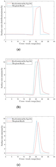
Figure A1.
Retrieval effect of Equation (14). (a) Surface rain distribution on rectangular rain; (b) surface rain distribution on trapezoidal rain; and (c) surface rain distribution on triangular rain.
Appendix B
This appendix is the retrieval method of some precipitation parameters that are not described in detail in the text.
According to the analysis in Section 2, the NRCS value at starts to decrease significantly due to the attenuation of the microwave by the bidirectional path. The value of can be obtained by taking a continuous average of the values of n NRCS sample values. When the radar resolution is 250 m, n is taken as 5. Calculate the mean and standard deviation of these 5 NRCS. If the sixth NRCS value is less than the mean of the previous 5 points minus three times the standard deviation, then the cross-track point corresponding to this NRCS is considered to be [27].
When the microwave emission is in the region of , the precipitation makes the NRCS decrease continuously. When the microwave continues to move forward to the region of , the path of the microwave in the rain and snow layers becomes shorter, and the NRCS begins to increase. So, the NRCS at is the smallest. Use the first and second derivatives of the NRCS to determine . Taking the sampling point as the center, calculate the average value of the NRCS of 5 points before and after the center to form a new average value function . The robust estimation of can be obtained by solving the first and second derivatives of .
Besides being closely related to , the retrieval of is also related to the freezing coefficient of the snow layer according to Equation (3). The snow rate of the snow layer is expressed as . is the average value of the snow rate of the snow layer:
Substitute Equation (3) into Equation (A3):
So, can be obtained by the ratio of to :
The average snow rate can be obtained by using the empirical relationship regressed to the NRCS simulation model [27]:
References
- Tang, J.; Chen, S.; Li, Z.; Gao, L. Mapping the Distribution of Summer Precipitation Types over China Based on Radar Observations. Remote Sens. 2022, 14, 3437. [Google Scholar] [CrossRef]
- Ju, X.; Huang, S.; Li, C.; Li, J.; Fan, S. Development of A Self-recording Per-minute Precipitation Dataset for China. J. Meteorol. Res. 2019, 33, 1157–1167. [Google Scholar] [CrossRef]
- Wang, H.; Zhong, P.; Zhu, F.; Lu, Q.; Xu, S.Y. The Adaptability of Typical Precipitation Ensemble Prediction Systems in the Huaihe River Basin, China. Stoch. Environ. Res. Risk Assess. 2021, 35, 1–15. [Google Scholar] [CrossRef]
- Yu, R.; Li, J.; Chen, H.; Yuan, W. Progress in Studies of the Precipitation Diurnal Variation over Contiguous China. J. Meteor. Res. 2014, 28, 877–902. [Google Scholar] [CrossRef]
- Fu, Y.F.; Lin, Y.H.; Liu, G.S.; Wang, Q. Seasonal Characteristics of Precipitation in 1998 over East Asia as Derived from TRMM PR. Adv. Atmos. Sci. 2003, 20, 511–529. [Google Scholar] [CrossRef]
- Xin, J.; Meng, K.; Wang, Y.; Dong, W.; Zhang, Y.C.; Yang, Z.F. Study on Rainfall Attenuation of Ka Band Satellite Remote Sensing Signals in Sanya. Radio Commun. Technol. 2022. [Google Scholar]
- Anagnostou, M.N.; Kalogiros, J.; Nikolopoulos, E.; Derin, Y.; Anagnostou, E.N.; Borga, M. Satellite Rainfall Error Analysis with the Use of High-Resolution X-Band Dual-Polarization Radar Observations over the Italian Alps; Springer International Publishing: Berlin, Germany, 2017; pp. 279–286. [Google Scholar] [CrossRef]
- Song, Z.J.; He, J.X.; Li, X.H.; Wang, H. Research Progress of Spaceborne Precipitation Measurement Radar Precipitation Products. Meteorol. Sci. Technol. 2018, 46, 631–637. [Google Scholar] [CrossRef]
- Durden, S.L.; Haddad, Z.S.; Kitiyakara, A.; Li, F.K. Effects of Nonuniform Beam Filling on Rainfall Retrieval for the TRMM Precipitation Radar. J. Atmos. Ocean. Technol. 1998, 15, 635. [Google Scholar] [CrossRef]
- Li, X.F.; Zhang, B.; Yang, X.F. Remote Sensing of Ocean Wind and Wave Fields by Spaceborne Synthetic Aperture Radar. J. Radars 2020, 9, 19. [Google Scholar] [CrossRef]
- Marzano, F.S.; Poccia, G.; Cantelmi, R.; Pierdicca, N.; Weinman, J.A.; Chandrasekar, V.; Mugnai, A. Potential of X-band Space-borne Synthetic Aperture Radar for Precipitation Retrieval over Land. In Proceedings of the IEEE International Geoscience & Remote Sensing Symposium, Barcelona, Spain, 23–28 July 2007; pp. 3694–3697. [Google Scholar] [CrossRef]
- Yağmur, N.; Tanık, A.; Tuzcu, A.; Musaoğlu, N.; Erten, E.; Bilgilioglu, B. Opportunities Provided by Remote Sensing Data for Watershed Management: Example of Konya Closed Basin. Int. J. Eng. Geosci. 2020, 5, 120–129. [Google Scholar] [CrossRef]
- Duysak, H.; Yiğit, E. Investigation of the Performance of Different Wavelet-based Fusions of SAR and Optical Images Using Sentinel-1 and Sentinel-2 Datasets. Int. J. Eng. Geosci. 2022, 7, 81–90. [Google Scholar] [CrossRef]
- Demirci, Ş.; Özdemir, C. An Investigation of the Performances of Polarimetric Target Decompositions Using GB-SAR Imaging. Int. J. Eng. Geosci. 2021, 6, 9–19. [Google Scholar] [CrossRef]
- Yiğit, E.; Demirci, Ş.; Özdemir, C. Clutter Removal in Millimeter Wave GB-SAR Images Using OTSU’s Thresholding Method. Int. J. Eng. Geosci. 2022, 7, 43–48. [Google Scholar] [CrossRef]
- Department of Aerospace Microwave Remote Sensing System, Institute of Aerospace Information Innovation, Chinese Academy of Sciences. Thirty Years of Spaceborne Synthetic Aperture Radar in China. J. Radars 2020, 9, 202. [Google Scholar]
- Deng, Y.K.; Yu, W.D.; Zhang, H.; Wang, W.; Liu, D.C.; Wang, Y. Forthcoming Spaceborne SAR Development. J. Radars 2020, 9, 1–33. [Google Scholar] [CrossRef]
- Zhang, R.N.; Jiang, X.P. Overall Design and on Orbit Verification of Environment-1c Satellite System. J. Radars 2014, 3, 7. [Google Scholar] [CrossRef]
- Zou, J.H.; Lin, M.S.; Zhang, Y.; Mu, B.; Guo, M.H.; Cui, S.X. Bin Matching of the Microwave Scatter Meter of HY-2 Satellite. J. Remote Sens. 2017, 21, 10. [Google Scholar] [CrossRef]
- The China Remote Sensing Satellite Ground Station Successfully Received the 03 Satellite Data of GF-3. Available online: https://www.cas.cn/yx/202204/t20220412_4831263.shtml (accessed on 12 April 2022).
- Marzano, F.S.; Mori, S.; Chini, M.; Pierdicca, N.; Montopoli, N.; Weinman, J.A. Potential of High-resolution Detection and Retrieval of Precipitation Fields from X-band Spaceborne Synthetic Aperture Radar over Land. Hydrol. Earth Syst. Sci. 2010, 15, 859–875. [Google Scholar] [CrossRef] [Green Version]
- Atlas, D.; Moore, R.K. The Measurement of Precipitation with Synthetic Aperture Radar. J. Atmos. Ocean. Technol. 1987, 4, 368–376. [Google Scholar] [CrossRef]
- Li, N.N.; Zhou, M.L.; Xie, Y.N. An Effective Echo Method for Precipitation Measurement by SAR at Different Doppler Velocities. Ind. Control Comput. 2018, 31, 3. [Google Scholar] [CrossRef]
- Luo, T.; Xie, Y.; Wang, R.; Yu, X. An Analytic Solution to Precipitation Attenuation Expression with Spaceborne Synthetic Aperture Radar Based on Volterra Integral Equation. Remote Sens. 2022, 14, 357. [Google Scholar] [CrossRef]
- Pichugin, A.P.; Spiridonov, Y.G. Spatial-distribution of Rainfall Intensity Recovery from Space Radar Images. Sov. J. Remote Sens. 1991, 8, 917–932. [Google Scholar]
- Weinman, J.A.; Marzano, F.S. An Exploratory Study to Derive Precipitation over Land from X-band Synthetic Aperture Radar Measurements. J. Appl. Meteorol. Climatol. 2006, 47, 562–575. [Google Scholar] [CrossRef] [Green Version]
- Marzano, F.S.; Weinman, J.A. Inversion of Spaceborne X-band Synthetic Aperture Radar Measurements for Precipitation Remote Sensing over Land. IEEE Trans. Geosci. Remote Sens. 2008, 46, 3472–3487. [Google Scholar] [CrossRef]
- Xie, Y.N.; Liu, Z.K.; An, D. An Algorithm to Retrieve Precipitation with Synthetic Aperture Radar. J. Meteorol. Res. 2016, 30, 401–411. [Google Scholar] [CrossRef]
- Melshelmer, C.; Alpers, W.; Gade, M. Investigation of Multifrequency/Multipolarization Radar Signatures of Rain Cells, Derived from SIR-C/X-SAR Data. In Proceedings of the IGARSS ‘96. 1996 International Geoscience and Remote Sensing Symposium, Lincoln, NE, USA, 31 May 1996; Volume 2, pp. 1370–1372. [Google Scholar] [CrossRef]
- Park, S.E. Variations of Microwave Scattering Properties by Seasonal Freeze/Thaw Transition in the Permafrost Active Layer Observed by ALOS PALSAR Polarimetric Data. Remote Sens. 2015, 7, 17135–17148. [Google Scholar] [CrossRef] [Green Version]
- Muhuri, A.; Manickam, S.; Bhattacharya, A.; Snehmani. Snow Cover Mapping Using Polarization Fraction Variation with Temporal RADARSAT-2 C-Band Full-Polarimetric SAR Data over the Indian Himalayas. IEEE J. Sel. Top. Appl. Earth Obs. Remote Sens. 2018, 11, 2192–2209. [Google Scholar] [CrossRef]
- Jordan, R.L.; Huneycutt, B.L.; Werner, M. The SIR-C/X-SAR Synthetic Aperture radar System. IEEE Trans. Geosci. Remote Sens. 1995, 33, 829–839. [Google Scholar] [CrossRef]
- Oh, Y.; Sarabandi, K.; Ulaby, F.T. An Empirical Model and An Retrieval Technique for Radar Scattering from Bare Soil Surfaces. IEEE Trans. Geosci. Remote Sens. 1992, 30, 370–381. [Google Scholar] [CrossRef]
- Ulaby, F.T.; Moore, R.K.; Fung, A.K. Microwave Remote Sensing: Active and Passive, 3rd ed.; Addison-Wesley Pub. Co.: London, UK, 1981; pp. 318–328. [Google Scholar]
- Yuter, S.E. Three-Dimensional Kinematic And Microphysical Evolution of Florida Cumulonimbus. Part II: Frequency Distributions of Vertical Velocity, Reflectivity, And Differential Reflectivity. Mon. Weather Rev. 1995, 123, 1921–1940. [Google Scholar] [CrossRef] [Green Version]
- Marzano, F.S.; Mori, S.; Weinman, J.A. Evidence of Rainfall Signatures on X-band Synthetic Aperture Radar Imagery over Land. IEEE Trans. Geosci. Remote Sens. 2010, 48, 950–964. [Google Scholar] [CrossRef]
- Huang, Y.T.; Guo, Y.G. Risk Assessment of Debris Flow Considering Rainfall Sensitivity: Taking Southeast Tibet as An Example. Chin. J. Geol. Hazards Prev. 2022. [Google Scholar]
- Shugar, D.H.; Jacquemart, M.; Shean, D.; Bhushan, S.; Upadhyay, K.; Sattar, A.; Schwanghart, W.; McBride, S.; Van Wyk de Vries, M.; Mergili, M.; et al. A Massive Rock and Ice Avalanche Caused the 2021 Disaster at Chamoli, Indian Himalaya. Science 2021, 373, 300–306. [Google Scholar] [CrossRef] [PubMed]
Publisher’s Note: MDPI stays neutral with regard to jurisdictional claims in published maps and institutional affiliations. |
© 2022 by the authors. Licensee MDPI, Basel, Switzerland. This article is an open access article distributed under the terms and conditions of the Creative Commons Attribution (CC BY) license (https://creativecommons.org/licenses/by/4.0/).