A Gamma-Log Net for Oil Spill Detection in Inhomogeneous SAR Images

Abstract

Due to the complexity of ocean environments, inhomogeneous phenomenon always exist in SAR images of oil spills on the sea surface. In order to address this issue, a universal parameter adaptive Gamma-Log net for detecting oil spills in inhomogeneous SAR images is proposed in this paper. The Gamma-Log net consists of an image feature division module, a correction parameter extraction module, a Gamma-Log correction module and a feature integration module. The normalized input image features are divided into four blocks for correction in the image feature division module. According to the input characteristics, the Gamma-Log correction input parameters are obtained in the correction parameter extraction module. Subsequently, an adaptive method is introduced to adjust the parameters independently by the network to improve efficiency. Then, the input features are corrected in the Gamma-Log correction module by Gamma correction and logarithmic correction. Both correction methods can adjust the gray imbalance in the image and change the overall gray value and contrast. The separated feature blocks are finally reunited together by the feature integration module. In order to avoid information loss, an attention mechanism is added to this module. In the experiments, by adding Gamma-Log Net to multiple semantic segmentation networks, the MIoU and dice indicators increased to some extent, and the HD distance(Hausdorff-95) decreased. Our work demonstrates that the Gamma-Log net can be helpful for oil spill detection in inhomogeneous SAR images.

1. Introduction

With the rapid development of marine transportation and the development of marine oilfields, the incidence of oil spill accidents is increasing. Marine oil spills can cause great harm to the surrounding marine environment, threatening animals and plants in the ocean, and causing huge economic losses to human production and life. Therefore, the detection and identification of the marine oil spill is particularly important. Marine oil spills are usually large in scope and not fixed in shape, so it is difficult to see all oil spills by manual means. Remote sensing can easily solve this problem.

Remote sensing technology can accurately observe a wide range of ground objects in a short time. Optical remote sensing based on the spectral response difference of ground objects can identify, determine and quantitatively extract the information of oil spill pollution, which can greatly improve the response ability and governance ability of oil spill events at sea. However, the optical remote sensing images are greatly affected by clouds. These clouds may cover the area to be observed, making researchers unable to obtain effective information in time, which will cause great obstacles to the rapid processing of offshore oil spill accidents. SAR (Synthetic Aperture Radar) satellite imaging is one of the most effective means of oil spill real-time monitoring, since the satellite can observe the ocean synchronously in all weather, all day, producing high resolution images at wide ranges. Such imagery are less affected by cloud and fog.

SAR can penetrate the atmosphere and cloud. Moreover, it can effectively identify the camouflage and cover, which is suitable for oil spill detection and can effectively identify the oil spill regions. These advantages are not achievable by visible light and infrared sensors. Therefore, SAR has become one of the effective sensor technologies for detecting marine oil spills and has been widely used in marine oil spill detection.

After an oil spill accident, the oil spilled on the sea surface will form oil film. The oil film on the sea surface will change the wave number spectrum of the sea surface tension attenuation Bragg shortwave. This will inhibit the backscattering echo signal received by SAR. Therefore, the oil film will appear as a dark low scattering region on SAR images. It looks quite different from the surrounding high roughness seawater environment. This is the theoretical basis for the detection and extraction of marine oil spills using SAR images. However, it is inefficient to manually label the location of oil spills in a large number of remote sensing images. Machine learning methods can solve this problem. Through the deep learning, the machine independently divides the oil spill area, and only a small part of the process is manual.

The improvement of SAR image segmentation can benefit from the domain adaptation method. Farahani [1] proposed a method based on self-encoders, which realized the fusion characteristics of synthetic aperture radar(SAR) and optics to benefit from their complementary information. The method aligned multi-temporal characteristics while reducing spectral and radiation differences, thus improving the accuracy of change detection. Stan [2] proposed a domain adaptation algorithm based on unsupervised learning. The algorithm uses the intermediate multimodal prototype distribution to minimize the distribution cross-domain differences in the shared embedding space. The proposed scheme is still competitive compared with the UDA algorithm based on joint domain model training. Zhang [3] proposed a domain adaptive neural network based on heterogeneous optics and SAR remote sensing image change detection. The scheme extracted heterogeneous depth features with the pseudo-Siam structure with non-shared weights. In order to bridge the gap between the source domain and the target domain in the unsupervised domain adaptation (UDA), Liu et al. [4] designed a novel edge-preserving self-determined progress contrast learning (MPSCL) model for cross-modal medical image segmentation. In that scheme, for the first time contrast learning was introduced to contrast learning to cope with the challenge of unsupervised domain adaptation in medical image segmentation. All the above work is useful for domain adaptation from an optical image to SAR image.

The research on marine oil spill detection can be divided into three categories: traditional image segmentation algorithms, machine learning and shallow neural network algorithms, and deep neural network algorithms. The most widely used method is based on threshold segmentation. The threshold is determined according to the bimodal histogram generated by oil-free surface and oil film covered surface. Based on the threshold, oil film is separated from the oil-free surface.The intensity-based threshold algorithm is an efficient means of calculation. Nirchio et al. [5] derived the wind intensity from the whole SAR image and the distance from the coastline to test the ability of SAR to reveal oil spills. Benito-Ortiz [6] determined the potential area of dark spots based on texture parameters, and used sea clutter statistical information to determine the adaptive threshold. Alattas [7] improved the threshold method of Gamma distribution, and combined the minimum cross entropy with a Gamma distribution function to form a double-layer threshold method to detect the oil spill of SAR images. Fan et al. [8] obtained the high frequency components of global features by a threshold segmentation method to weaken the influence of point noise in SAR images, and then superimposed these features to the downsampling layers, so that the model can make more accurate decisions. However, these threshold methods are easily affected by the sea surface speckle noise, resulting in a low accuracy of oil film segmentation.

With the support of a large data volume, the detection algorithm based on neural networks can usually achieve better detection results. However, these networks need many parameter settings. Liu et al. [9] proposed a texture index calculated from the four texture features of the gray level co-occurrence matrix for texture analysis, and used a machine learning method to extract the crude oil leakage area. Lyu [10] used a gray level co-occurrence matrix and Tamura features to extract the required features from SAR images, and improved the accuracy of oil spill detection with the help of an extreme learning machine model. Yekeen et al. [11] used a novel deep learning instance segmentation model for marine oil spill detection based on the Mask-RCNN model, which has a better performance than other traditional machine learning models and semantic segmentation models. Baek [12] used the support vector machine (SVM), random forest (RF) and deep neural network (DNN) models to compare and analyze the performance of oil spill classification in different polarization modes of X-band synthetic aperture radar (SAR) images. Taravat [13] used a pulse coupled neural network and a multi-layer perceptron for image segmentation, and subsequently used a filter based on Weibull multiplication model to filter out false targets for improving the performance of the model. Ronci [14] innovatively used an adversarial loss function to train convolutional neural networks, and achieved promising results. According to the geometric characteristics of an oil spill, Wang et al. [15] used the long-term and short-term memory network to process the memory information, thus obtaining the relationship between characteristics and influencing factors. Using these factors, he established the initial system model and oil spill behavior monitoring model.

Shaban et al. [16] proposed a new deep learning framework based on a 23-layer convolutional neural network and a five-stage U-Net structure for the oil spill event recognition task of highly imbalanced datasets. This set-up improved the accuracy and the Dice score. The above methods were used to process the original SAR oil spill image, but there was no correction for inhomogeneous SAR images. The SAR images are highly speckled. Thus, the inhomogeneous areas in the images will make the oil spill characteristics unclear to be detected. The first step of oil spill monitoring scheme is usually the detection of dark strata [17]. If the spill area is missed in this step, it is difficult to be detected in subsequent steps.

Due to the complexity of the marine environment and the multi-interpretation of oil spill characteristics, many marine phenomena may also lead to the enhancement or attenuation of SAR image echo signals. This in turn creates interference, resulting in the misclassification of oil spill detection in SAR images. The phenomenon is usually shown as too bright or too dark regions in SAR images. Low backscatter pixel values may be associated with sea clutter, ground clutter, floating oil or analogues [17], whereas high backscatter pixel values may lead to background blurring.

SAR data is highly speckled and inhomogeneous areas widely appear in various SAR images. The inhomogeneous areas will have a great impact on the identification and segmentation of marine oil spill areas. The Gamma correction method can enhance or weaken the image gray value by changing the parameter gamma value, so as to increase the image contrast. Logarithmic correction is better in enhancing images with low overall contrast and low gray value. Therefore, this paper proposes a general module for adaptive adjustment of inhomogeneous SAR images. This module will perform Gamma correction and Logarithmic correction on image features, so as to improve the image segmentation effect. The segmentation effect is verified on six commonly used networks, including UNet [18], UNet++ [19], and Attention-UNet [20], etc.

2. Materials and Methods

2.1. Databases and Processing

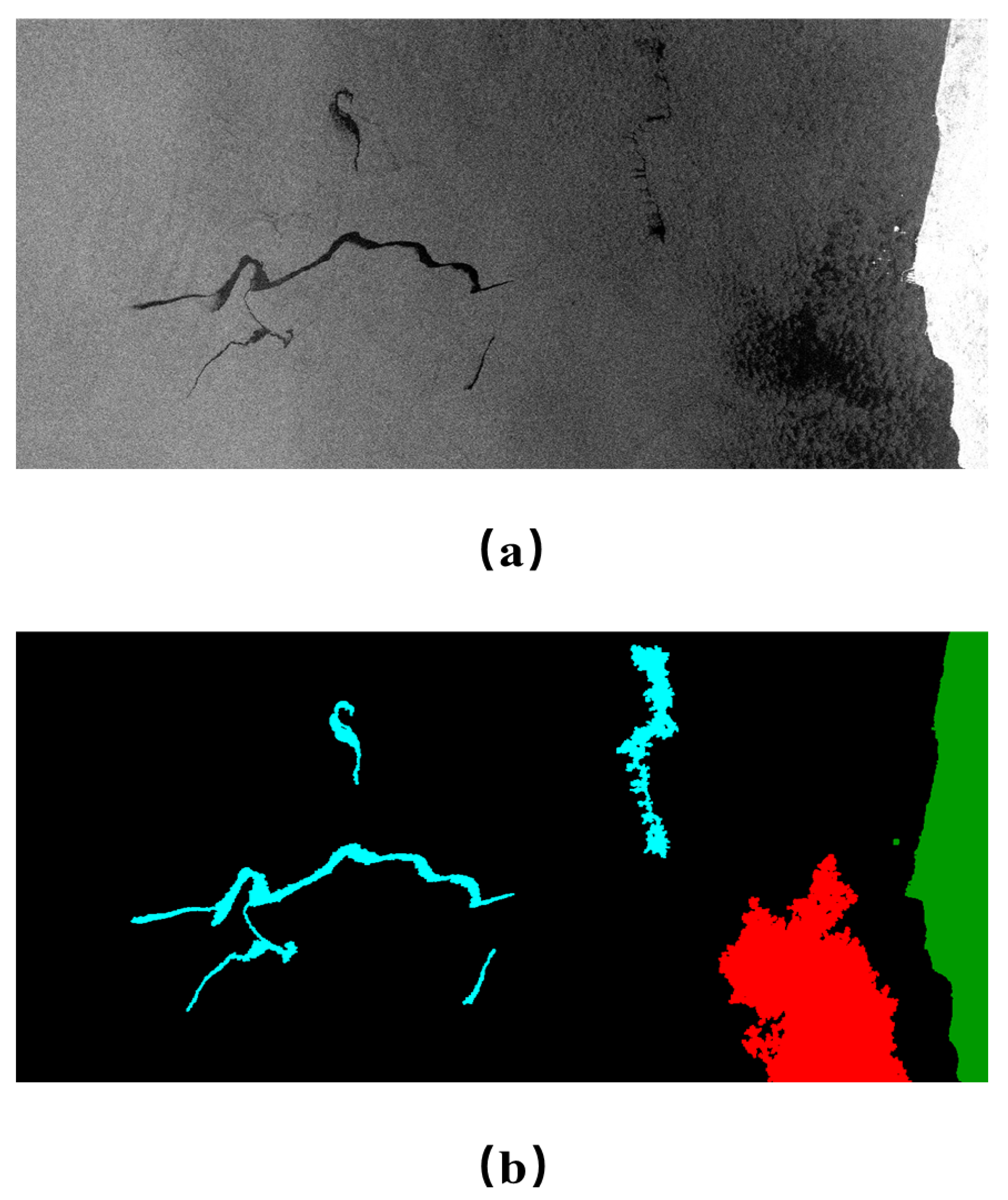
The experiments in this paper use C band SAR data. The oil-spill-detection-dataset was based on [21,22]. The original dataset is set to 1002 training set images and 110 test set images. The resolution of images is 1250 × 650 × 3. In the original oil spill dataset, the image includes instances of an oil spill, oil spill look-alike, ships, land and sea, and generates three-dimensional labels for all instances. Cyan, red, brown, Green and black masks represent the oil spill, oil spill look-alike, ships, land and sea. Figure 1a shows an example of a SAR image in the dataset. Figure 1b is an example of a 3-D mask for SAR images. The dataset also provides one-dimensional labels for segmentation and classification. In

Table 1. The mask of each instance and the number of pixels occupied in the dataset.

Class	3-D Masks	1-D Labels
Sea surface	Black	0
Oil spill	Cyan	1
Look-alike	Red	2
Ship	Brown	3
Land	Green	4

, the set of 0, 1, 2, 3, 4, 5 denotes sea surface, oil spill, oil spill look-alike, ship and land, respectively. The proportion of oil spill pixels in the dataset is 20%, which makes the dataset balanced. In this paper, the training set images are randomly divided into a training dataset and verification dataset according to the ratio of 8:2, and the image size was cut to 256 × 256. This paper pays more attention to the improvement of oil spill area segmentation accuracy.

2.2. Gamma-Logarithmic Correction and Gamma-Log Module

2.2.1. Basic Knowledge

Image contrast correction methods are diverse, and include methods such as histogram equalization, linear stretching, Gamma correction, Logarithmic correction, etc. After the histogram equalization transformation, the gray level of the image decreases and some details disappear, which makes it difficult for the neural network to fully obtain the details of the image. Since the linear stretching method applies the same stretching function to all gray values, the linear relationship between input and output will be affected by the maximum and minimum gray values of input. If the maximum and minimum values in the image deviate too far, the correction effect of the image will be very poor. Gamma correction and Logarithmic correction are both nonlinear stretching transformations, which are suitable for oil spill images with nonlinear data. At the same time, Logarithmic correction can solve the problem of a small dynamic range and missing some details in Gamma correction. Therefore, in this paper, we use Gamma correction and Logarithmic correction to correct inhomogeneous SAR images.

Threshold segmentation is an important image segmentation method, and is also the most commonly used method in oil spill detection. Image threshold segmentation can accurately segment the target by analyzing the gray characteristics of the region to be segmented and setting the threshold. At the same time, the image threshold segmentation can retain some isolated regions by selecting the appropriate threshold, so that the segmented target can retain more details. However, when the pixel values in the image are relatively concentrated, the gamma correction method can inadvertently stretch the pixel values of the image. The whole image gray value is the sum of each pixel gray values. Logarithmic correction has better performance when the overall image has low pixel values and contrast.

Gamma distribution is the cumulative distribution of multiple independent and identically distributed exponential distribution variables, and is also closely related to Beta and Chi-square distribution. The probability density function of the Gamma distribution [23] is defined by Equation (1),

$$f(x,\mu ,N)=\frac{2q}{\mu }\frac{N^N}{\Gamma \left(N\right)}{\left(\frac{qx}{\mu }\right)}^{2N-1}{e}^{-N{(qx/\mu )}^2},q=\frac{\Gamma (N+0.5)}{\Gamma \left(N\right)\sqrt{N}}$$

(1)

where x is the intensity value of image pixels, and $\mu$ is the average value of the distribution. The shape of the gamma distribution depends on the parameter N. Traditionally, the $\Gamma \left(\right)$ is defined by Equation (2),

$$\Gamma \left(x\right)={\int }_0^{\infty }{x}^{\alpha -1}{e}^{-x}dx$$

(2)

where $\alpha$ denotes a positive parameter.

The images on the dataset are affected by the marine environment and other factors, resulting in great differences in image intensity. This may in turn result in poor oil spill segmentation performance. In order to improve the generalization of the marine oil spill segmentation task, the inhomogeneous images need to be adjusted. In fact, Gamma correction and Logarithmic correction are typical methods to adjust the overall intensity and contrast of input images. Therefore, through Gamma correction and Logarithmic correction, the Gamma-Log module adjusts the inhomogeneous images to make the image features able to be learned better in the network. Thus, the network can better distinguish the oil spill area in the corrected image. The traditional Gamma correction is defined by Equation (3),

$$Y=K{X}^{\gamma }.X,Y\in R^{H\times W},\gamma >0$$

(3)

where X and Y denote normalized input images and output images, respectively; H and W represent the height and width of input images, respectively; K denotes a constant; and $\gamma$ denotes a positive parameter. The value of $\gamma$ determines the gray mapping between the input image and the output image. In other words, it determines whether to enhance the low gray value area or enhance the high gray value area.

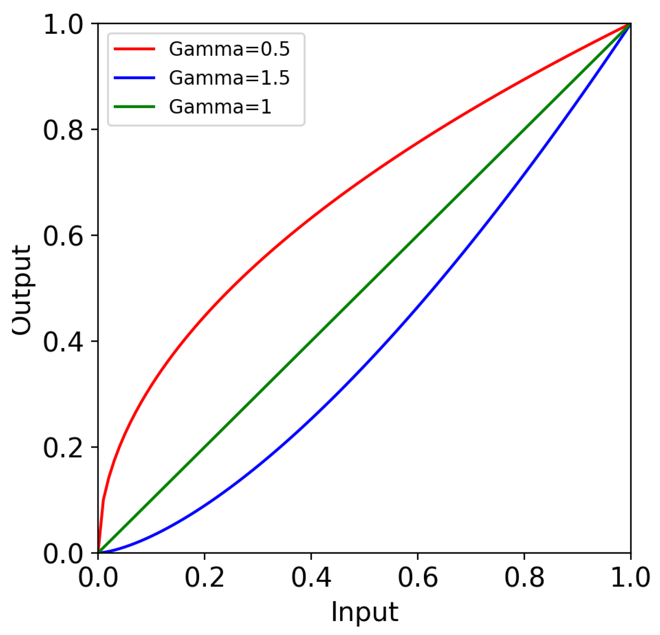
The Gamma correction curve is shown in Figure 2. When $\gamma$ > 1, the dynamic range of the low gray value regions becomes smaller, and the dynamic range of the high gray value of the regions becomes larger. It reduces the contrast of low gray value regions and raises the contrast of high gray value regions. At the same time, the overall gray value of the image is reduced. A darker output image is generated. As shown in Figure 2, when $\gamma$ < 1, in the low gray value regions, the dynamic range becomes larger, and the image contrast is enhanced. In the high gray value region, the dynamic range becomes smaller, and the image contrast decreases. The overall gray value of the image is thus improved. A brighter output image is generated. When $\gamma$ = 1, the original image is not changed. The image enhancement effect of Gamma correction is obvious when the image contrast is low and the overall brightness value is high.

The traditional Logarithmic correction is usually defined by Equation (4),

$$Y=Clog(1+X).$$

(4)

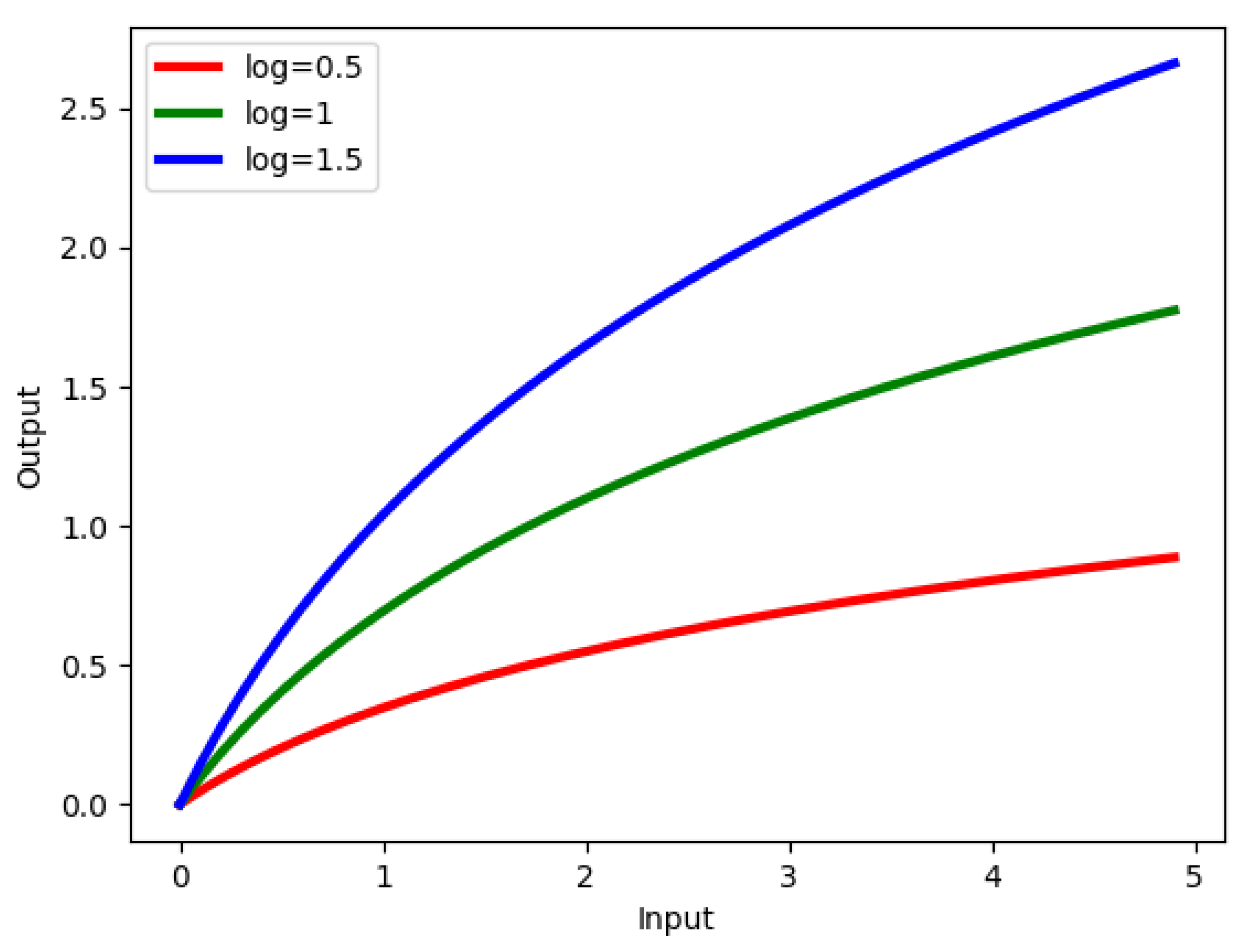
where X and Y are normalized input images and output images, respectively; C is a constant. In Figure 3, when log takes different values, the maximum of the output will be different. Logarithmic correction partially increases the low gray values of the image and partially reduces high pixel values. This emphasizes the low gray part of the image and achieves the purpose of image correction. Logarithmic correction is better for image enhancement with low overall contrast and low gray value.

2.2.2. Gamma-Log Net

In order to ensure that the image contrast can be adjusted to the best values, Gamma correction and Logarithmic correction usually require significant manual tuning to set the corresponding parameter values. The enhancement effect of the corrected image is usually evaluated by human visual perception, and then people determine whether the setting of correction parameters is appropriate. This evaluation method is not applicable in deep learning because it is very inefficient. Therefore, a parameter adaptive method is proposed in this paper. By limiting the parameter values in the range 0 and 2, the network can adaptively evaluate which correction method is used. Subsequently, the network takes the cross entropy loss between the predicted and ground truth images to evaluate the correction effect of image features. The feature maps in the deep convolutional neural network can be regarded as images and can be mapped to their corresponding input images. Thus, Gamma and Logarithmic corrections can be used to adjust the intensity of the feature map. Convolutional neural networks can adaptively change parameter values with the change of input image features, so as to adjust the inhomogeneous images.

In order to avoid manually selecting the best gamma value for each feature graph, self-learning is introduced and a correction parameter extraction module is proposed. The main principle of the correction parameter extraction module is to adaptively learn the value of each feature map according to the global pixel intensity distribution. The learned values will be used as input parameters for Gamma correction and Logarithmic correction. In addition, the Gamma-Log Net divides each feature map into several blocks so that different regions on each feature map can adaptively adjust their feature values. Since the values of different feature channels and blocks are not the same, the Gamma-Log Net adds spatial and channel attention mechanisms to focus the network on particular channels and local areas.

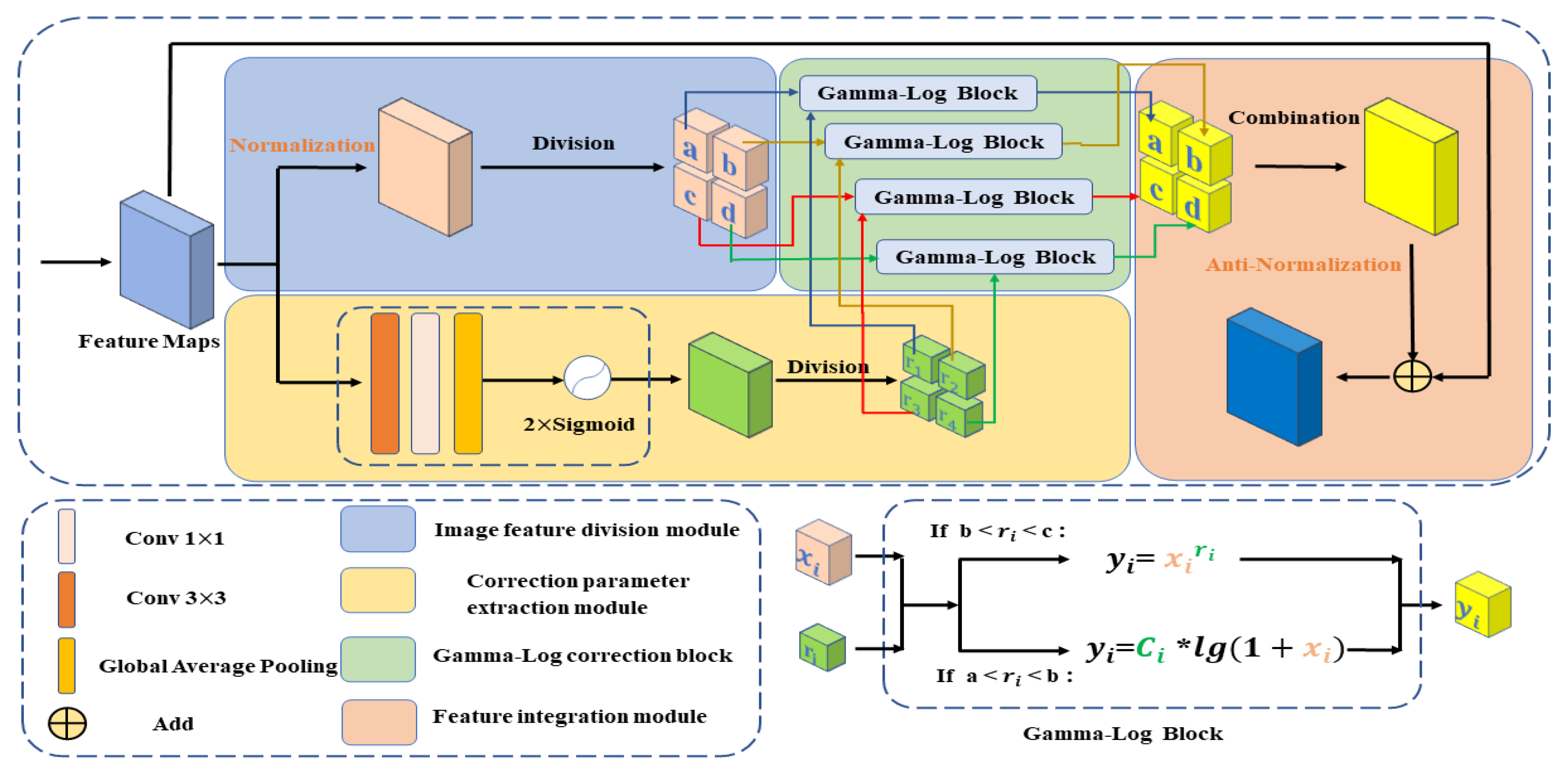
The overall structure of the Gamma-Log Net is shown in Figure 4. The processing of input feature blocks is divided into two parts. First, the input feature map is input into the image feature block module. The image feature block module is shown in the blue region of Figure 4. The feature map needs to be normalized first, and the range of eigenvalues is limited between 0 and 1, in order to conveniently correct image features. Dark regions may appear anywhere in inhomogeneous images, so normalized features are divided into four quadrants for correction.

Secondly, the input image features will be fed into the correction parameter extraction module. The correction parameter extraction module is shown on the yellow region of Figure 4. The network needs to obtain the global pixel intensity distribution of feature blocks to determine whether and where features need to be corrected. In order to obtain the global strength distribution of each layer, feature blocks are input into the global average pooling layer. The global average pooling operation is shown in Equation (5).

$${\mathrm{O}}_{\mathrm{n}}^{\mathrm{m}}=\frac{1}{\mathrm{H}\times \mathrm{W}}\times \sum _{\mathrm{p}=1}^{\mathrm{H}}\sum _{\mathrm{q}=1}^{\mathrm{W}}{\mathrm{I}}_{\mathrm{n}}^{\mathrm{m}},\mathrm{m}=1,2,.\mathrm{p},\mathrm{n}=1,2,.\mathrm{q}$$

(5)

where I and O represent the input and output characteristic blocks, respectively. H and W represent the length and width of image features in each layer. ${\mathrm{I}}_{\mathrm{n}}^{\mathrm{m}}$ denotes the input characteristics of the n-th channel in the m-th batch. ${\mathrm{O}}_{\mathrm{n}}^{\mathrm{m}}$ denotes the output characteristics of the n-th channel in the m-th batch. $\mathrm{p}$ denotes the maximum of the batches, and $\mathrm{q}$ represents the maximum of channels.

$$Sigmoid\left(x\right)=\frac{1}{1+e^{-x}}$$

(6)

After the global average pooling, the feature map passes through the convolution layers of 3 × 3 and 1 × 1 to obtain the parameter block with length of 2, width of 2 and channel number of n. In addition, an improved sigmoid activation function is also proposed. In Equation (6), x denotes the input of activation function. Each value in the parameter block is limited in the range 0 and 2. Then, the parameter block is also divided into 2 × 2 blocks, corresponding to the output of the image feature block module. This ensures that each one of the 2 × 2 feature blocks in each layer has a value corresponding to it, and so both of them can be input into the correction module at the same time.

Taking the feature block a as an example, feature block a and parameter block ${\mathrm{r}}_{\mathrm{i}}$ are input into the Gamma-Log block module. The Gamma-Log block module is shown on the green region of Figure 4. In the Gamma-Log block module, four feature blocks need to be input into four Gamma-Log blocks for correction. In Gamma-Log blocks, the input parameter ${\gamma }_{\mathrm{i}}$ needs to be evaluated. When a $<{\gamma }_{\mathrm{i}}<$ b, where a = 0 and b = 1, the Logarithmic correction method is used. The feature block is taken as X, and the parameter block is taken as C. C is obtained by mathematical calculation through parameter $\gamma$. They are substituted into Equation (2) to obtain the feature map after Logarithmic correction. When b $<{\gamma }_{\mathrm{i}}<$ c, where b = 1 and c = 2, the Gamma correction method is used. The feature block is taken as X, and the parameter block is taken as $\gamma$. They are then substituted into Equation (1) to obtain the feature map after Gamma correction.

After the Gamma-Log block correction module, the four feature blocks are recombined into a whole feature map in the feature integration module. The feature integration module is shown on the orange region of Figure 4. The whole feature map is inversely normalized to remove the range limitation of 0 to 1. In addition, the input gradient flow is reintroduced to avoid information loss shown in Equation (7). ⨁ denotes that the input gradient flow is added to the characteristics of recombination.

$$O=I+[max(I)-min(I\left)\right]\times X+min\left(I\right)$$

(7)

The I in the formula is the input feature of the Gamma-Log module. O is the output feature after denormalization and addition of the attention mechanism. X is the feature block corrected by the Gamma-Log block. By adding Gamma-Log blocks to the backbone network, the intensity gap in the feature map can be adjusted to improve the segmentation effect.

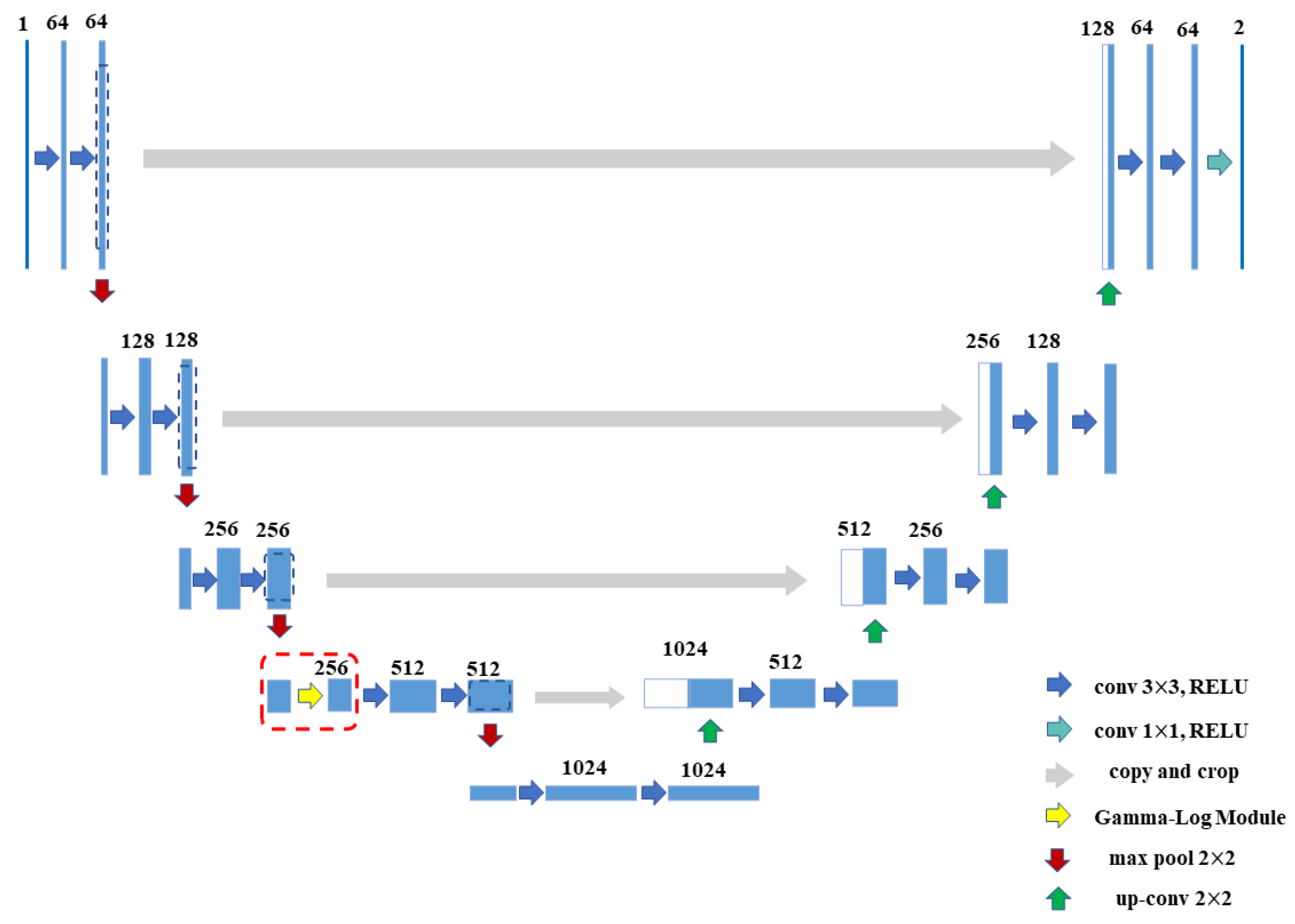
In six network models, we test the performance of the Gamma-Log Net architecture, taking UNet as an example. UNet is a encoder-decoder structure as a whole, which includes five down-sampling paths, five up-sampling paths and a bottleneck bridge. UNet obtains multi-scale image information in down-sampling. In order to avoid losing details, each up-sampling path has a skip component to obtain the features of the down-sampling path. The shallow convolution focuses on the texture information of the image, but each down-sampling operation will lead to the loss of edge information. Deep convolution pays more attention to deep features. In order to achieve the balance between both, the Gamma-Log Net architecture is placed behind the pooling layer of the third down-sampling operation and connected to the fourth down-sampling operation, as shown in Figure 5.

3. Results and Discussion

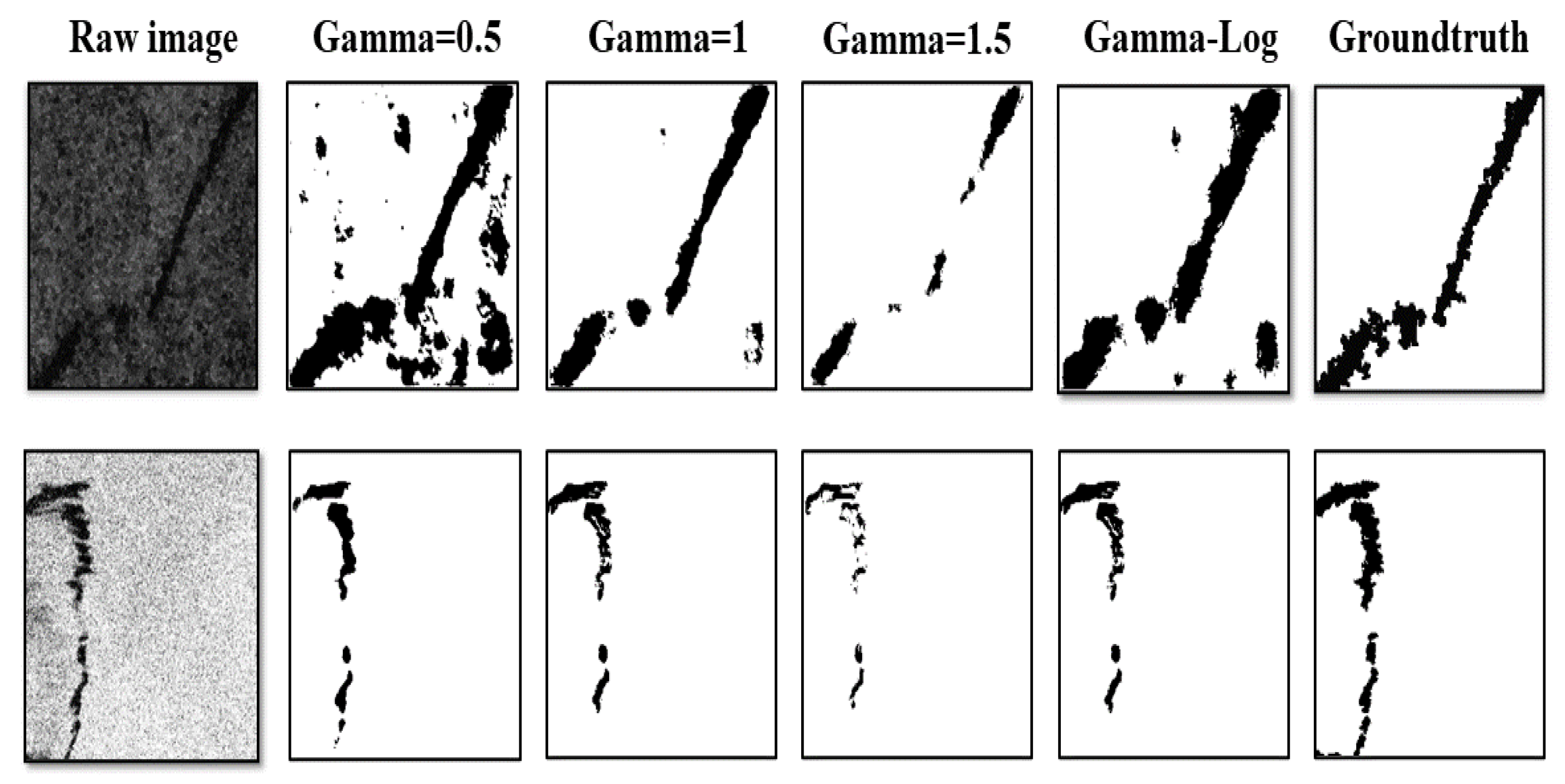
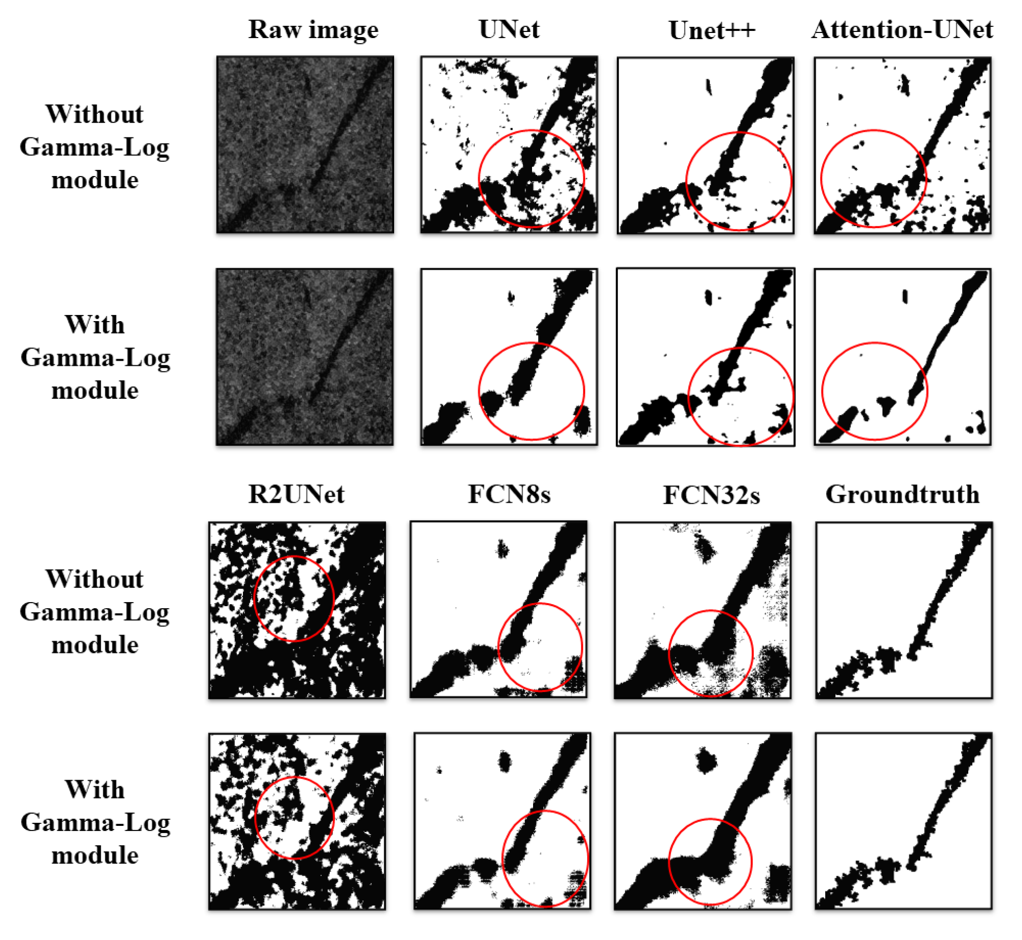
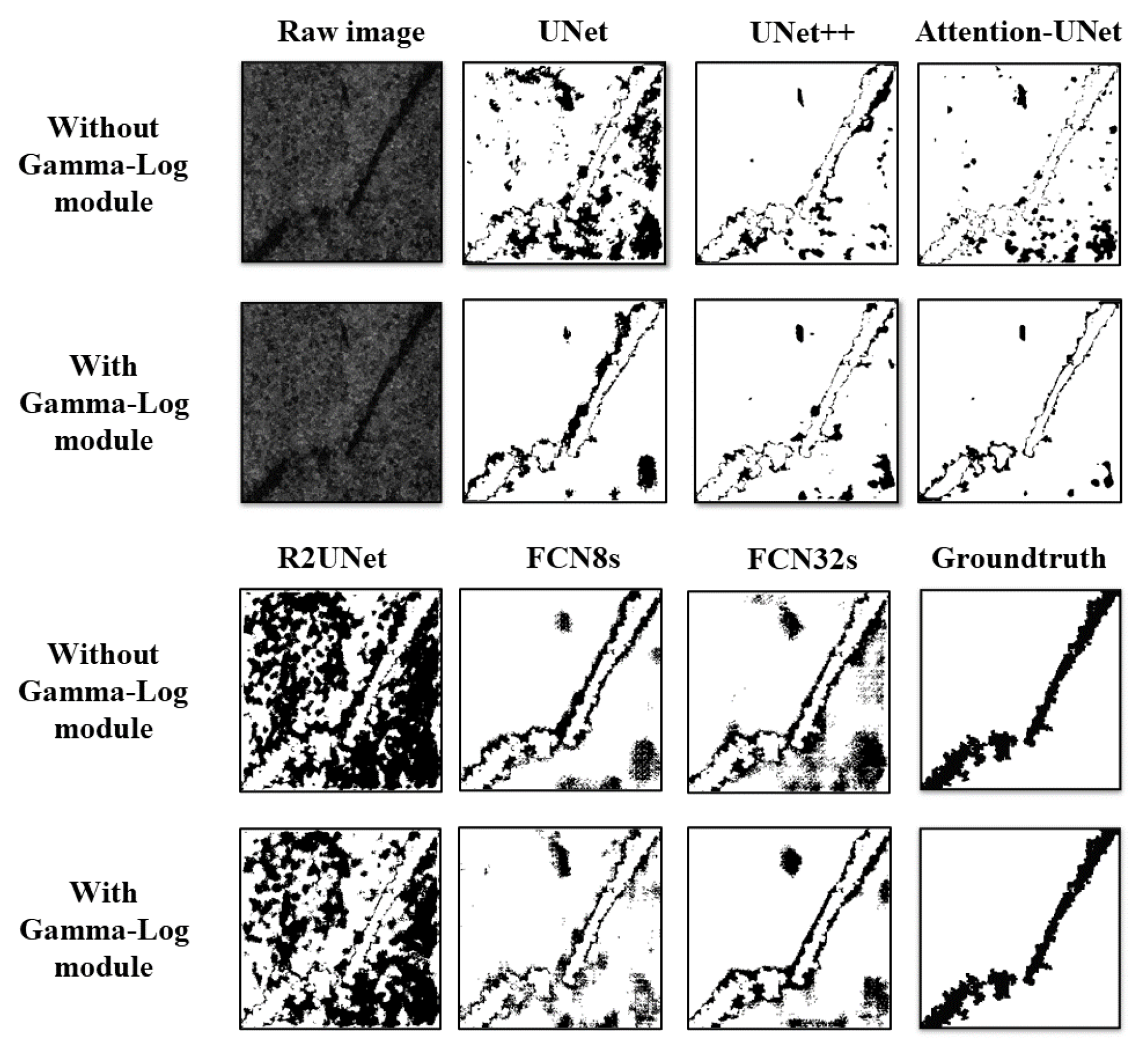
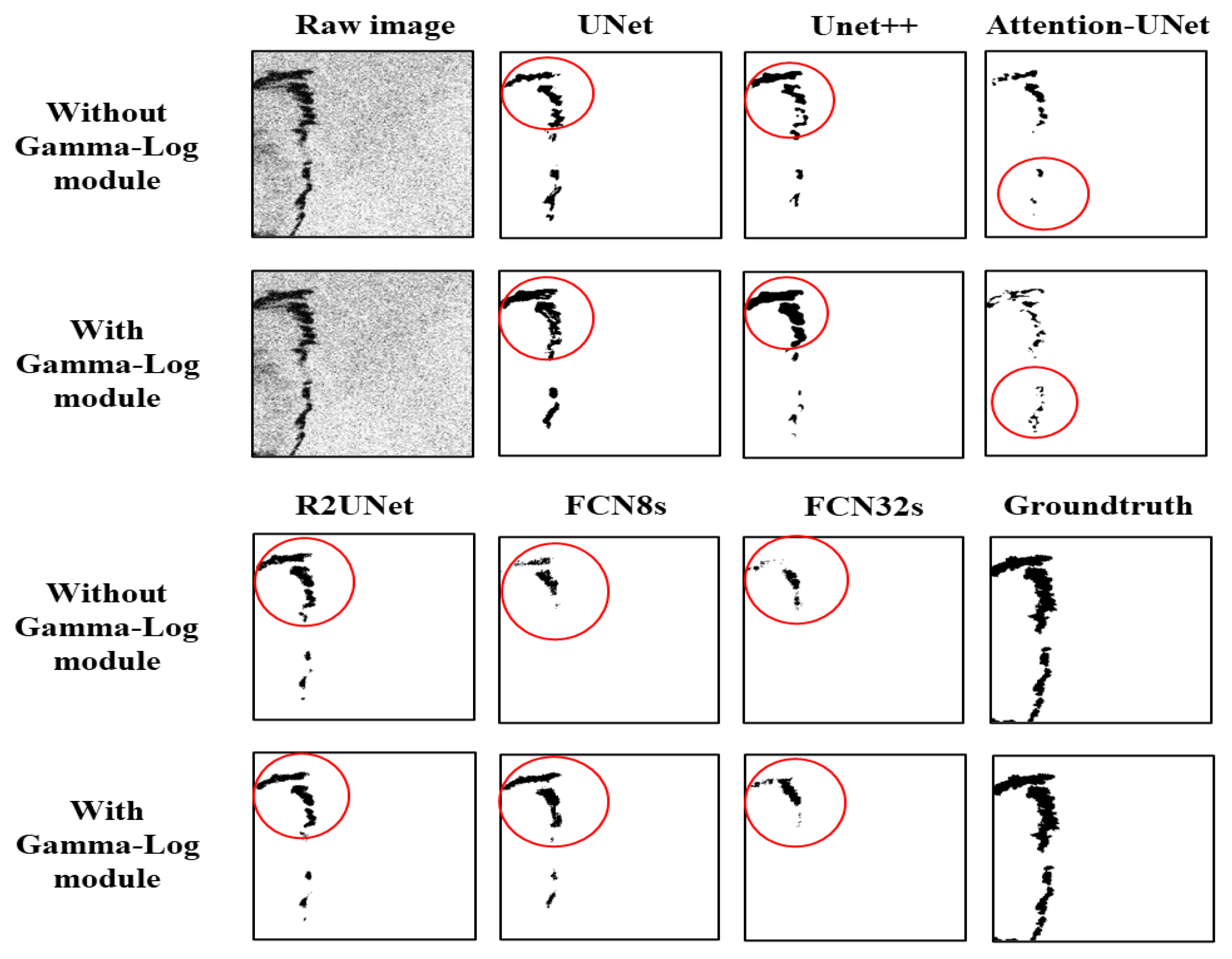
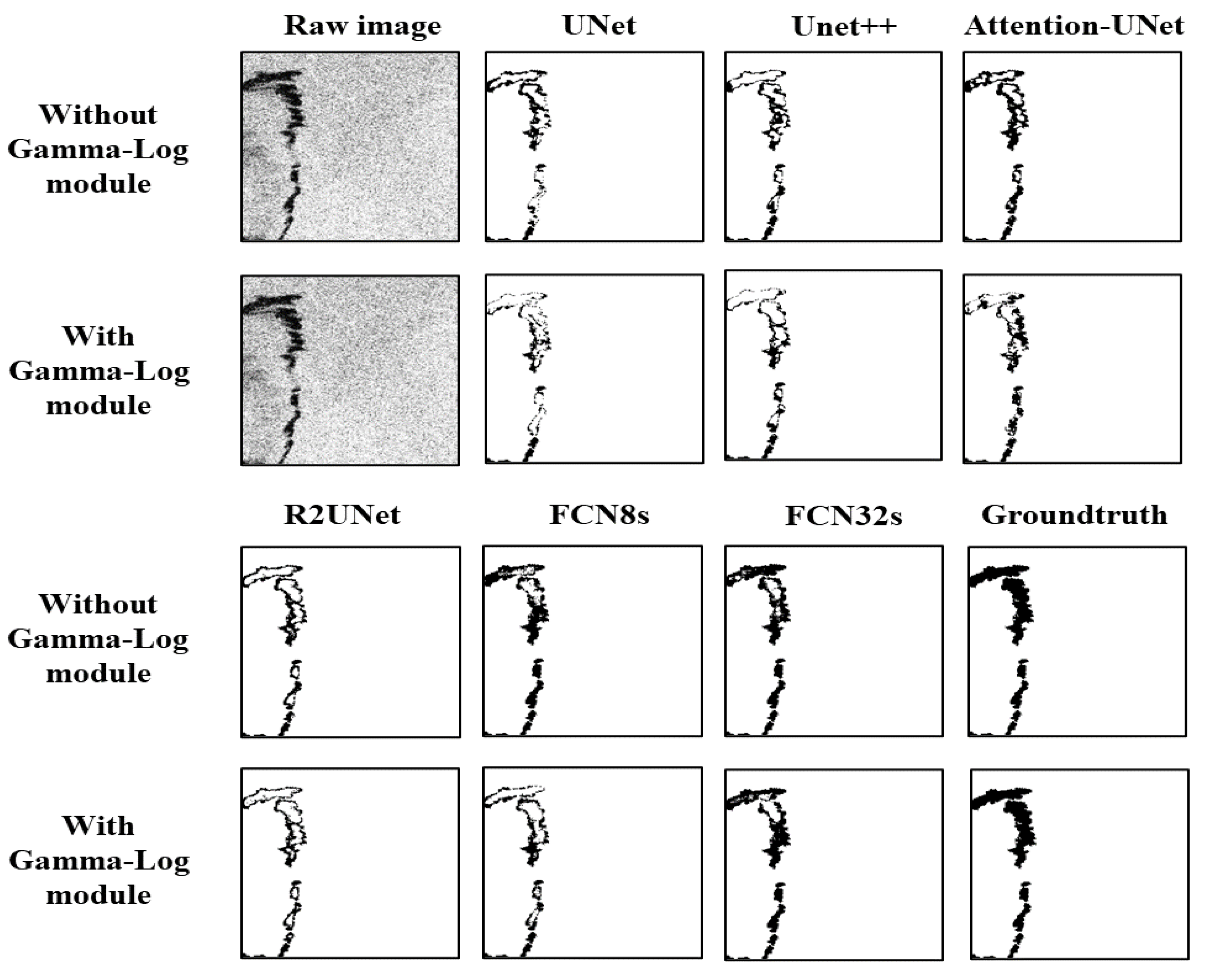
The experiments in this paper are executed in the pytorch environment on NVIDIA 2080ti GPU. In Figure 6, we compared the prediction results using the Gamma-Log correction method compared to using only the Gamma correction method. From the images in the second, third, fourth and fifth column, it can be found that when different images are corrected, the result of using only Gamma correction is worse than that of using the Gamma-Log correction. After adding the Gamma-Log Net architecture to multiple network frameworks, the trained model is tested, and the results are demonstrated in Figure 7. It can be observed from the Figure 7 that the whole original test image is dark, and the boundaries between the background and some oil spill areas are difficult to distinguish. This is consistent with the performance of heterogeneous SAR images. In UNet, Attention-UNet and FCN8s as can be observed from Figure 7, and wrongly detected areas have been significantly reduced. This shows that the segmentation accuracy has been greatly improved. In Figure 8, after adding Gamma-Log Net, it can be seen that the difference between the model predicted image and the ground truth in Figure 7 has decreased in each network structure. After adding the Gamma-Log Net architecture to multiple network frameworks, the trained model is tested, and the results are demonstrated in Figure 9. It can be observed from Figure 9 that the background is bright. UNet, UNet++ and FCN8s with Gamma-Log Net can identify more oil spill areas compared to the models without Gamma-Log Net. After adding the Gamma-Log Net architecture to R2UNet, the wrongly detected area is confined to a small part of the image and the segmentation accuracy is improved slightly. The Equation (8) is to illustrate how to generate an image of the difference between the prediction and the ground truth.

$$O=I_{\mathrm{predict}}\cup I_{\mathrm{groundruth}}-I_{\mathrm{predict}}\cap I_{\mathrm{groundruth}}$$

(8)

The $I_{\mathrm{predict}}$ in the Equation (8) denotes the model prediction results. The $I_{\mathrm{groundruth}}$ denotes the ground truth. In addition, the O denotes the output images. In the Equation (8), the union and intersection between the model prediction results and the ground truth are calculated. The output of the Equation (8) is the difference between the predicted results and the ground truth. The ground truth and the prediction result of each model in Figure 7 and Figure 9 are the inputs to Equation (8). After calculation by Equation (8), the corresponding outputs are shown in Figure 8 and Figure 10, respectively. In

Table 2. Comparison of the area where the predictions differ from the ground truth in six networks before and after adding the Gamma-Log Net architecture in Figure 7.

Models	Pixels	Pixels (with Gamma-Log)	Percent	Percent (with Gamma-Log)
UNet	13,868	3031 (−8173)	23.6458%	5.0353% (−18.6105%)
UNet++	4834	4077 (−757)	8.2099%	6.9240% (−1.2859%)
Attention-UNet	5250	3293 (−1957)	8.9161%	5.3903% (−3.5258%)
R2-UNet	36,978	29,202 (−7776)	63.2081%	49.9069% (−13.30312%)
FCN8s	8341	7946 (−395)	14.2377%	13.5630% (−0.6747%)
FCN32s	11,796	8467 (−3329)	20.1479%	14.4609% (−5.687%)

and

Table 3. Comparison of the area where the predictions differ from the ground truth in six networks before and after adding the Gamma-Log Net architecture in Figure 9.

Models	Pixels	Pixels (with Gamma-Log)	Percent	Percent (with Gamma-Log)
UNet	2011	1464 (−547)	3.1442%	2.3088% (−0.8354%)
UNet++	2081	1764 (−317)	3.2484%	2.7676% (−0.4808%)
Attention-UNet	2699	2016 (−683)	4.1726%	3.1504% (−1.0222%)
R2-UNet	2019	2215 (+196)	3.1545%	3.4502% (+0.2957%)
FCN8s	2956	2122 (−834)	4.5519%	3.3106% (−1.2413%)
FCN32s	3115	3076 (−39)	4.7849%	4.7295% (−0.0554%)

, This column named pixel is the statistics of the difference in pixels between the predictions and the ground truth. These areas are marked as black in Figure 8 and Figure 10. The percentages are the proportions of these pixels in the entire image. In Table 2, we can observe comparisons of the pixels and the percentages before and after adding Gamma-Log Net. In UNet, R2UNet and FCN32s with Gamma-Log Net, the area of differences between the model predicted image and the ground truth has been significantly reduced. The area of differences in UNet++, Attention-UNet and FCN8s has been also reduced slightly. The Figure 10 presents the results of the differences between the model predicted image in Figure 9 and the ground truth before and after adding Gamma-Log Net. In Table 3, we can see comparisons of the pixels and the percentages before and after adding Gamma-Log Net. In UNet, UNet++, Attention-UNet and FCN8s with Gamma-Log Net, the area of differences between the model predicted image and the ground truth has been reduced. The area of differences in FCN32s has been reduced slightly. The differences in R2UNet are slightly increased.

In order to evaluate the oil spill segmentation effect accurately, the metrics MIoU(Mean Intersection over Union), aver-Dice(average Dice coefficient) and aver-HD(average Hausedorf Distance-95) are introduced. Intersection over Union (IoU) is essentially a method to quantify the overlap percentage between target and prediction mask. Specifically, it refers to the ratio of the number of pixels in the common area of the target mask and the prediction mask to the total number of pixels in the image. MIoU is the average IoU for each category.

$$\mathrm{MloU}=\frac{1}{k+1}\sum _{i=0}^k\frac{p_{ii}}{{\sum }_{j=0}^k{p}_{ij}+{\sum }_{j=0}^k{p}_{ji}-p_{ii}}$$

(9)

The calculation of the above metric is performed in two steps. In the first step, for each category, the ratio of intersection and union is calculated. This proportion of molecules is the correct number predicted under this category; a larger range of denominators means that this category is predicted as the sum of other categories. The second step is to average the calculation results of all categories.

MIoU is used to calculate the average cross-over ratio between test samples and real samples. The general definition formula of MIoU is shown in Equation (10),

$$\mathrm{MloU}=\frac{\mathrm{TP}}{\mathrm{FP}+\mathrm{FN}+\mathrm{TP}}$$

(10)

where TP is the number of true positives. FP is the number of false positives. TN is the number of true negatives. FN is the number of false negatives.

The MIoU results before and after adding the Gamma-Log Net architecture to six networks are shown in

Table 4. Comparison of MIoU and the IoU’s standard deviations in six networks before and after adding the Gamma-Log Net architecture.

Models	MIoU	MIoU (with Gamma-Log)	$\mathit{\sigma }$	$\mathit{\sigma }$ (with Gamma-Log)
UNet	94.1289%	95.5747% (+1.45%)	0.1679	0.1441 (−0.0238)
UNet++	95.1891%	95.555% (+0.37%)	0.1507	0.1441 (−0.0066)
Attention-UNet	95.0631%	95.5794% (+0.52%)	0.1521	0.1424 (−0.0097)
R2-UNet [24]	91.9062%	92.3326% (+0.43%)	0.2041	0.1988 (−0.0052)
FCN8s [25]	94.941%	95.0833% (+0.14%)	0.1731	0.1520 (−0.0211)
FCN32s	93.8884%	94.2886% (+0.4%)	0.1873	0.1768 (−0.0105)

. In the six network models, UNet++ and Attention-UNet have good performance, with MIoU value higher than 95%. After adding the Gamma-Log Net architecture to all network frameworks, Unet’s MIoU value increased by 1.45%. Attention-UNet was the second best, with its MIoU value increasing by 0.52%. R2UNet, FCN32s and UNet ++ also have a good improvement. Their MIoU values increased by 0.43%, 0.4% and 0.37%, respectively. Finally, the MIoU value of FCN8s increased by 0.14%. Since using the average value makes it difficult to reflect the overall deviation of a set of data, the standard deviation is introduced. By comparing the change of standard deviation before and after adding the Gamma-Log Net, the change of the outliers in the overall data can be obtained. In the six network models, we added the Gamma-Log Net architecture to all network frameworks. It can be observed that the standard deviations of UNet and FCN8s decreased the most by 0.0238 and 0.0211, respectively. FCN32s, Attention-UNet, UNet++ and R2UNet also have a good performance. Their MIoU’s standard deviations value decreased by 0.0105, 0.0097, 0.0066 and 0.0052, respectively.

The Dice coefficient is a metric for measuring the similarity of sets. It is used to calculate the similarity of two samples. The value range of the Dice coefficient is between 0 and 1. The general calculation formula of the Dice Coefficient is shown in Equation (11).

$$s=\frac{2|X\bigcap Y|}{\left|X\right|+\left|Y\right|}$$

(11)

X represents the prediction samples. Y represents the ground truth. $|X\bigcap Y|$ is the intersection between X and Y, which is the intersection between the predicted results and the ground truth. $\left|X\right|$ and $\left|Y\right|$ represent the number of elements of X and Y. The molecular coefficient in Equation (11) is 2, which is due to the repeated calculation of common elements between X and Y. The molecular coefficient is multiplied by 2 to ensure that the value range of the denominator is between 0 and 1 after the repeated calculation. According to the above definition of the Dice coefficient, the following formula can be obtained by converting Equation (11) into the confusion matrix shown in Equation (12):

$$Dice=\frac{2TP}{2TP+FP+FN}$$

(12)

The aver-Dice coefficient results before and after adding the Gamma-log Net architecture to six networks are shown in

Table 5. Comparison of aver-Dice coefficients and the Dice’s standard deviations before and after adding the Gamma-Log Net architecture in six networks.

Models	aver-Dice	aver-Dice (with Gamma-Log)	$\mathit{\sigma }$	$\mathit{\sigma }$ (with Gamma-Log)
UNet	95.7667%	96.8563% (+1.09%)	0.1421	0.1217 (−0.0204)
UNet++	96.5669%	96.8379% (+0.27%)	0.1274	0.1228 (−0.0046)
Attention-UNet	96.4845%	96.8801% (+0.40%)	0.1284	0.1202 (−0.0082)
R2-UNet	93.8788%	94.2124% (+0.33%)	0.1817	0.1769 (−0.0048)
FCN8s	96.3396%	96.5044% (+0.16%)	0.1518	0.1273 (−0.0245)
FCN32s	95.223%	95.6453% (+0.42%)	0.1705	0.1578 (−0.0127)

. Among the six network models, the highest aver-Dice values are achieved for UNet++ and Attention-UNet, reaching over 96%. After adding the Gamma-Log Net architecture to all network frameworks, UNet improves the most with its aver-Dice coefficient increasing by 1.09%. Attention-UNet and FCN32s had the second best improvements with their aver-Dice coefficients increasing by 0.4% and 0.42%, respectively. Finally, the other three network models UNet++, R2-UNet and FCN8s have improved their aver-Dice coefficients after adding the Gamma-Log Net architecture by 0.27%, 0.33% and 0.16%, respectively. The aver-Dice values of R2UNet, UNet++ and FCN8s increased by 0.33%, 0.27% and 0.16%, respectively. In the six network models, after adding the Gamma-Log Net architecture to all network frameworks, the Dice’s standard deviations of UNet and FCN8s decreased the most by 0.0204 and 0.0245, respectively. FCN32s, Attention-UNet, UNet++ and R2UNet also have a good performance. Their Dice’s standard deviations value decreased by 0.0127, 0.0082, 0.0046 and 0.0048, respectively.

HD (the Hausedorf Distance-95) is an indicator to measure the accuracy of boundary segmentation. The Dice coefficient is sensitive to the segmented internal filling, while the Hausdorff distance is sensitive to the segmented boundary. The general definition for HD (Hausdorff-95) is shown in Equation (13).

$$d_H(X,Y)=max\left\{\underset{x\in X}{max}\underset{y\in Y}{min}(x,y),\underset{y\in Y}{max}\underset{x\in X}{min}d(x,y)\right\}$$

(13)

The difference between the predicted target region boundary and the real target region boundary is $d_H(X,Y)$. 95% HD is obtained by multiplying $d_H(X,Y)$ by 95%. 95% HD is similar to the maximum HD. The purpose of using this confidence interval is to eliminate the influence of the minimum subset. It can be inferred from Equation (13) that HD (Hausdorff-95) can be used to characterize the maximum deviation between the predicted boundary and the ground truth boundary of segmentation in the image.

The aver-HD results before and after adding Gamma-Log Net architecture to six networks are shown in

Table 6. Comparison of aver-HD before and after adding the Gamma-Log Net architecture in six networks.

Models	aver-HD	aver-HD (with Gamma-Log)
UNet	3.127644	2.616432 (−0.51)
UNet++	2.694023	2.77241 (+0.083)
Attention-UNet	2.860443	2.848871 (−0.011)
R2-UNet	3.768138	3.641564 (−0.126574)
FCN8s	2.763118	2.769389 (+0.0062)
FCN32s	2.771686	2.72986 (−0.042)

.

After adding the Gamma-log Net architecture to the six network frameworks, the aver-HD of most network models has been reduced to some extent. This shows that our Gamma-Log Net architecture can indeed produce prediction results close to the ground truth. Among them, the aver-HD value of UNet decreased the most by 0.51. Furthermore, the aver-HD of R2UNet, Attention-UNet and FCN32s also decreased by 0.126574, 0.011 and 0.042, respectively.

However, the HD values of UNet++ and FCN8s increased. This is because when the corrected feature blocks are combined together, there is a large gap in the characteristics at the splicing edge of different feature blocks. This will form the basis of our further work on the problem.

In our experiments, six network structures were used to verify the improvement of the oil spill segmentation task due to adding the Gamma-Log module. The prediction results of six network models before and after adding the Gamma-Log correction module are shown in Figure 7, and the prediction results are compared with the ground truth.

MIoU is a commonly used metric in semantic segmentation. After adding the Gamma-Logarithm correction module, the MIoU of the model has been improved, which means that the network has improved the segmentation accuracy of the oil spill images. At the same time, the Dice coefficient value has increased, which means the segmentation results are more similar to the ground truth. After the Gamma-Log correction module is added to the network, the Hausdorff-95 value is reduced, which means that the outliers at the boundary of the segmentation result are reduced, and the segmentation accuracy at the boundary is improved. Therefore, the changes of the above three indicators fully demonstrate that the addition of Gamma-Log correction module will improve the segmentation results of marine oil spill images.

4. Conclusions

This paper proposes a Gamma-Log Net architecture to adjust the inhomogeneous SAR images which have low contrast, thus making it difficult to distinguish between the background and targets. The Gamma-Log Net architecture adaptively performs Gamma and Logarithmic corrections on input features to improve image inhomogeneity, thus enabling more efficient detection of oil spill images. Comprehensive qualitative and quantitative empirical evaluations have validated that a variety of state-of-the-art models using the proposed Gamma-log Net architecture can improve in the oil spill detection of inhomogeneous SAR images.

References

1. Farahani, M.; Mohammadzadeh, A. Domain adaptation for unsupervised change detection of multisensor multitemporal remote-sensing images. Int. J. Remote Sens. 2020, 41, 3902–3923. [Google Scholar] [CrossRef]
2. Stan, S.; Rostami, M. Unsupervised Model Adaptation for Continual Semantic Segmentation. In Proceedings of the AAAI Conference on Artificial Intelligence, Online, 2–9 February 2021. [Google Scholar]
3. Zhang, C.; Feng, Y.; Hu, L.; Tapete, D.; Pan, L.; Liang, Z.; Cigna, F.; Yue, P. A domain adaptation neural network for change detection with heterogeneous optical and SAR remote sensing images. Int. J. Appl. Earth Obs. Geoinf. 2022, 109, 102769. [Google Scholar] [CrossRef]
4. Liu, Z.; Zhu, Z.; Zheng, S.; Liu, Y.; Zhou, J.; Zhao, Y. Margin Preserving Self-Paced Contrastive Learning Towards Domain Adaptation for Medical Image Segmentation. IEEE J. Biomed. Health Inform. 2022, 26, 638–647. [Google Scholar] [CrossRef] [PubMed]
5. Nirchio, F.; Sorgente, M.; Giancaspro, A.; Biamino, W.; Parisato, E.; Ravera, R.J.; Trivero, P. Automatic detection of oil spills from SAR images. Int. J. Remote Sens. 2005, 26, 1157–1174. [Google Scholar] [CrossRef]
6. Benito-Ortiz, M.C.; de la Mata-Moya, D.; Jarabo-Amores, M.P.; Maganto-Pascual, M.; del Hoyo, P.G. Multi-resolution Technique-Based Oil Spill Look-Alikes Detection in X-Band SAR Data. In Proceedings of the Advances in Intelligent Systems and Computing, Chengdu, China, 1–3 June 2018. [Google Scholar]
7. Alattas, R. Oil spill detection in SAR images using minimum cross-entropy thresholding. In Proceedings of the 2014 7th International Congress on Image and Signal Processing, Cherbourg, France, 30 June–2 July 2014; pp. 709–713. [Google Scholar]
8. Fan, Y.; ping Rui, X.; Zhang, G.; Yu, T.; Xu, X.; Poslad, S. Feature Merged Network for Oil Spill Detection Using SAR Images. Remote Sens. 2021, 13, 3174. [Google Scholar] [CrossRef]
9. Liu, P.; Li, Y.; Liu, B.; Chen, P.; Xu, J. Semi-Automatic Oil Spill Detection on X-Band Marine Radar Images Using Texture Analysis, Machine Learning, and Adaptive Thresholding. Remote Sens. 2019, 11, 756. [Google Scholar] [CrossRef] [Green Version]
10. Lyu, X. Oil Spill Detection Based on Features and Extreme Learning Machine Method in SAR Images. In Proceedings of the 2018 3rd International Conference on Mechanical, Control and Computer Engineering (ICMCCE), Huhhot, China, 14–16 September 2018; pp. 559–563. [Google Scholar]
11. Yekeen, S.T.; Balogun, A.L.B. Automated Marine Oil Spill Detection Using Deep Learning Instance Segmentation Model. In Proceedings of the ISPRS—International Archives of the Photogrammetry, Remote Sensing and Spatial Information Sciences, Online, 31 August–2 September 2020; pp. 1271–1276. [Google Scholar]
12. Baek, W.K.; Jung, H.S. Performance Comparison of Oil Spill and Ship Classification from X-Band Dual- and Single-Polarized SAR Image Using Support Vector Machine, Random Forest, and Deep Neural Network. Remote Sens. 2021, 13, 3203. [Google Scholar] [CrossRef]
13. Taravat, A.; Frate, F.D. Weibull Multiplicative Model And Machine Learning Models for Full-Automatic Dark-Spot Detection from Sar Images. In Proceedings of the ISPRS—International Archives of the Photogrammetry, Remote Sensing and Spatial Information Sciences, Melbourne, Australia, 25 August–1 September 2013; pp. 421–424. [Google Scholar]
14. Ronci, F.; Avolio, C.; Donna, M.D.; Zavagli, M.; Piccialli, V.; Costantini, M. An adversarial learning approach for oil spill detection from SAR images. In Proceedings of the 2020 IEEE Radar Conference (RadarConf20), Florence, Italy, 21–25 September 2020; pp. 1–4. [Google Scholar]
15. Wang, R.; Zhu, Z.; hua Zhu, W.; Fu, X.; Xing, S. A Dynamic Marine Oil Spill Prediction Model Based on Deep Learning. J. Coast. Res. 2021, 37, 716–725. [Google Scholar] [CrossRef]
16. Shaban, M.; Salim, R.; Khalifeh, H.A.; Khelifi, A.; Shalaby, A.M.; El-Mashad, S.Y.; Mahmoud, A.M.; Ghazal, M.; El-Baz, A.S. A Deep-Learning Framework for the Detection of Oil Spills from SAR Data. Sensors 2021, 21, 2351. [Google Scholar] [CrossRef] [PubMed]
17. Benito-Ortiz, M.C.; de la Mata-Moya, D.; Jarabo-Amores, M.P.; del Rey-Maestre, N.; del Hoyo, P.G. Generalized Gamma Distribution SAR Sea Clutter Modelling for Oil Spill Candidates Detection. In Proceedings of the 2019 27th European Signal Processing Conference (EUSIPCO), A Coruna, Spain, 2–6 September 2019; pp. 1–5. [Google Scholar]
18. Ronneberger, O.; Fischer, P.; Brox, T. U-Net: Convolutional Networks for Biomedical Image Segmentation. In Proceedings of the International Conference on Medical Image Computing and Computer-Assisted Intervention, Munich, Germany, 5–9 October 2015. [Google Scholar]
19. Zhou, Z.; Siddiquee, M.M.R.; Tajbakhsh, N.; Liang, J. UNet++: A Nested U-Net Architecture for Medical Image Segmentation. In Deep Learning in Medical Image Analysis and Multimodal Learning for Clinical Decision Support, Proceedings of the 4th International Workshop, DLMIA 2018, and 8th International Workshop, ML-CDS 2018, Held in Conjunction with MICCAI 2018, Granada, Spain, 20 September 2018; Springer: Cham, Switzerland, 2018; Volume 11045, pp. 3–11. [Google Scholar]
20. Oktay, O.; Schlemper, J.; Folgoc, L.L.; Lee, M.J.; Heinrich, M.P.; Misawa, K.; Mori, K.; McDonagh, S.G.; Hammerla, N.Y.; Kainz, B.; et al. Attention U-Net: Learning Where to Look for the Pancreas. arXiv 2018, arXiv:1804.03999. [Google Scholar]
21. Krestenitis, M.; Orfanidis, G.A.; Ioannidis, K.; Avgerinakis, K.; Vrochidis, S.; Kompatsiaris, Y. Oil Spill Identification from Satellite Images Using Deep Neural Networks. Remote Sens. 2019, 11, 1762. [Google Scholar] [CrossRef] [Green Version]
22. Krestenitis, M.; Orfanidis, G.A.; Ioannidis, K.; Avgerinakis, K.; Vrochidis, S.; Kompatsiaris, Y. Early Identification of Oil Spills in Satellite Images Using Deep CNNs. In Proceedings of the International Conference on Multimedia Modeling, Thessaloniki, Greece, 8–11 January 2019. [Google Scholar]
23. Zaart, A.E.; Ziou, D.; Wang, S.; Jiang, Q. Segmentation of SAR images. Pattern Recognit. 2002, 35, 713–724. [Google Scholar] [CrossRef]
24. Alom, M.Z.; Hasan, M.; Yakopcic, C.; Taha, T.M.; Asari, V.K. Recurrent Residual Convolutional Neural Network based on U-Net (R2U-Net) for Medical Image Segmentation. arXiv 2018, arXiv:1802.06955. [Google Scholar]
25. Long, J.; Shelhamer, E.; Darrell, T. Fully convolutional networks for semantic segmentation. In Proceedings of the 2015 IEEE Conference on Computer Vision and Pattern Recognition (CVPR), Boston, MA, USA, 7–12 June 2015; pp. 3431–3440. [Google Scholar]
Figure 1. (a) SAR image examples, including oil spill, oil spill look-alike, sea and land. (b) 3-D mask of each instance in the sample image.
Remotesensing 14 04074 g001
Figure 2. Gamma correction curve when γ takes different values. When the constant K value is 1, the function curve with γ value of 0.5 is red. The function curve with γ value of 1 is green. The function curve with γ value of 1.5 is blue.
Remotesensing 14 04074 g002
Figure 3. Logarithmic correction curve when the constant C takes different values. When the base number of the logarithmic function is the natural logarithm e, the function curve with C value of 0.5 is red. The function curve with C value of 1 is green. The function curve with C value of 1.5 is blue.
Remotesensing 14 04074 g003
Figure 4. Overall structure of the Gamma-Log module. In the virtual block, when the input parameter b < γ i < c, the image feature block is corrected by the Gamma function. When a < γ i < b, the Logarithmic correction is applied to image feature blocks.
Remotesensing 14 04074 g004
Figure 5. UNet network structure with Gamma-Log module.
Remotesensing 14 04074 g005
Figure 6. The comparison chart of prediction results after adding Gamma-Log correction module in UNet. The first column is the original image. The second column, the third column and the fourth column are the prediction results when the gamma value is 0.5, 1 and 1.5. The images in the fifth column are the prediction results with Gamma-Log Net architecture. The images in the last column are the ground truth.
Remotesensing 14 04074 g006
Figure 7. The comparison chart of prediction results before and after adding Gamma-Log correction module in each network structure. The first column is the original image, and each subsequent column corresponds to the prediction results of different networks. The images in the top row are the prediction results without Gamma-Log correction module. The images in the bottom row are the prediction results with Gamma-Log correction module. The images in the last column are the ground truth.
Remotesensing 14 04074 g007
Figure 8. The comparison chart of differences between the model predicted image and the ground truth before and after adding Gamma-Log correction module in each network structure. The first column is the original image, and each subsequent column corresponds to the prediction results of different networks. The images in the top row are the differences between the model predicted image and the ground truth without Gamma-Log correction module. The images in the bottom row are the differences with Gamma-Log correction module. The images in the last column are the ground truth.
Remotesensing 14 04074 g008
Figure 9. The comparison chart of prediction results before and after adding the Gamma-Log correction module in each network structure. The first column is the original image, and each subsequent column corresponds to the prediction results of different networks. The images in the top row are the prediction results without Gamma-Log correction module. The images in the bottom row are the prediction results by using the Gamma-Log correction module. The images in the last column are the ground truth.
Remotesensing 14 04074 g009
Figure 10. The comparison chart of differences between the model predicted image and the ground truth before and after adding the Gamma-Log correction module in each network structure. The first column is the original image, and each subsequent column corresponds to the prediction results of different networks. The images in the top row are the differences between the model predicted image and the ground truth without Gamma-Log correction module. The images in the bottom row are the differences between the predictions and the ground truth with Gamma-Log correction module. The images in the last column are the ground truth.
Remotesensing 14 04074 g010