Increasing the Lateral Resolution of 3D-GPR Datasets through 2D-FFT Interpolation with Application to a Case Study of the Roman Villa of Horta da Torre (Fronteira, Portugal)

Abstract

The approach presented in this work uses an interpolation methodology to densify 3D-GPR datasets to sharpen the results obtained in GPR surveys carried out in an archaeological environment. It allows the estimation of missing data from the combined use of mathematical transforms, such as the Fourier and curvelet transforms, and predictive filters. This technique makes it possible to calculate the missing signal simply by meeting two requirements: the data in the frequency domain must be limited in a range of values and must be able to be represented by a distribution of Fourier coefficients (verified conditions). The INT-FFT algorithm uses an open-access routine (Suinterp, Seismic Unix) to interpolate the GPR B-scans based on seismic trace interpolation. This process uses automatic event identification routines by calculating spatial derivatives to identify discontinuities in space by detecting very subtle changes in the signal, thus allowing for more efficient interpolation without artifacts or signal deterioration. We successfully tested the approach using GPR datasets from the Roman villa of Horta da Torre (Fronteira, Portugal). The results showed an increase in the geometric sharpness of the GPR reflectors and did not produce any numerical artifacts. The tests performed to apply the methodology to GPR-3D data allowed for assessing the interpolation efficiency, the level of estimation of missing data, and the level of information lost when we chose to increase the distance between B-scans in the acquisition stage.

1. Introduction

1.1. Ground-Penetrating Radar in Archaeologic Exploration

Geophysical methods to prospect the subsurface in an archaeological environment are essential for remote sensing studies using noninvasive and nondestructive techniques. These features can increase knowledge about an archaeological site and play an essential role in site planning, which can make heritage protection endeavors more effective.

Among the various methods available, ground-penetrating radar (GPR) is one of the most common electromagnetic methods used in archaeological geophysics. It has become more popular since 1970 [1] due to its advantages of quick data acquisition and high resolution. This method allows the determination of the spatial distribution of buried structures in the ground, such as walls, ditches, floors, cavities, and even water levels. We obtain this information by propagating an electromagnetic wave (EMW) in the ground with a known frequency. The typical frequency values for archaeological prospection vary between 200 MHz and 1.6 GHz [2]. Among several requirements to apply GPR to obtain the data, there is a need to control some aspects of the acquisition, the field procedure, and the parameterization of the equipment. In acquisitions in 3D mode through parallel B-scans, an adequate parameterization includes controlling a set of requirements such as the orientation of the B-scans, the number of samples per trace, trace separation, temporal range, and gain adjustment. The number of B-scans to be acquired is also one of the selected parameters that have consequences on the acquisition time and the quality of the results. A longer distance between B-scans reduces the acquisition time but can prevent the detection of reflectors corresponding to buried structures. The task of defining these parameters requires careful consideration.

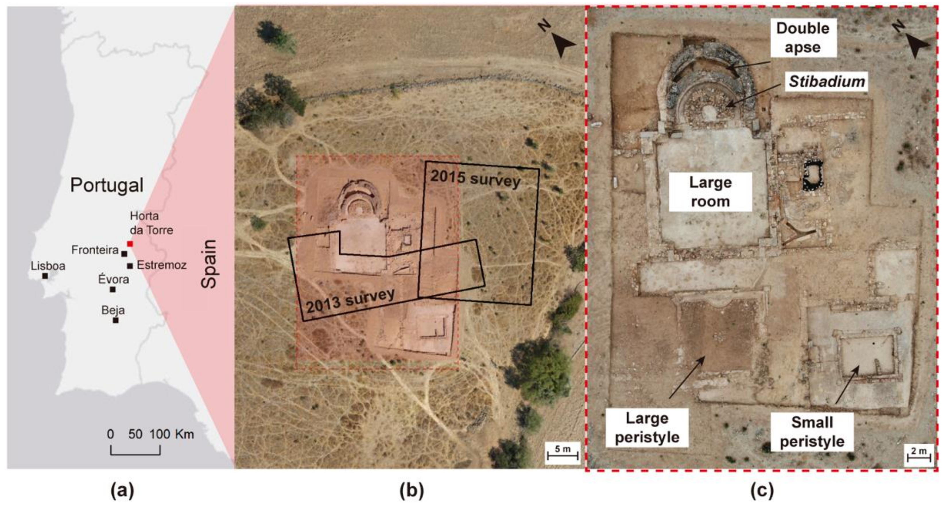
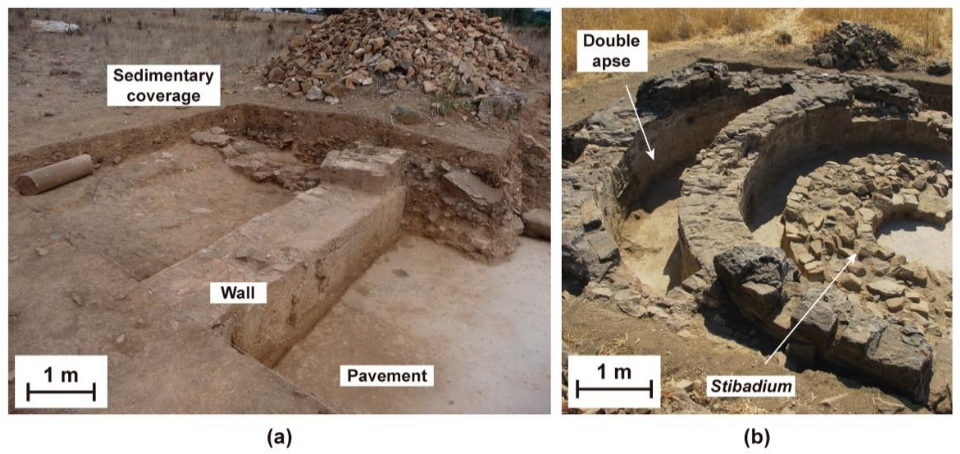
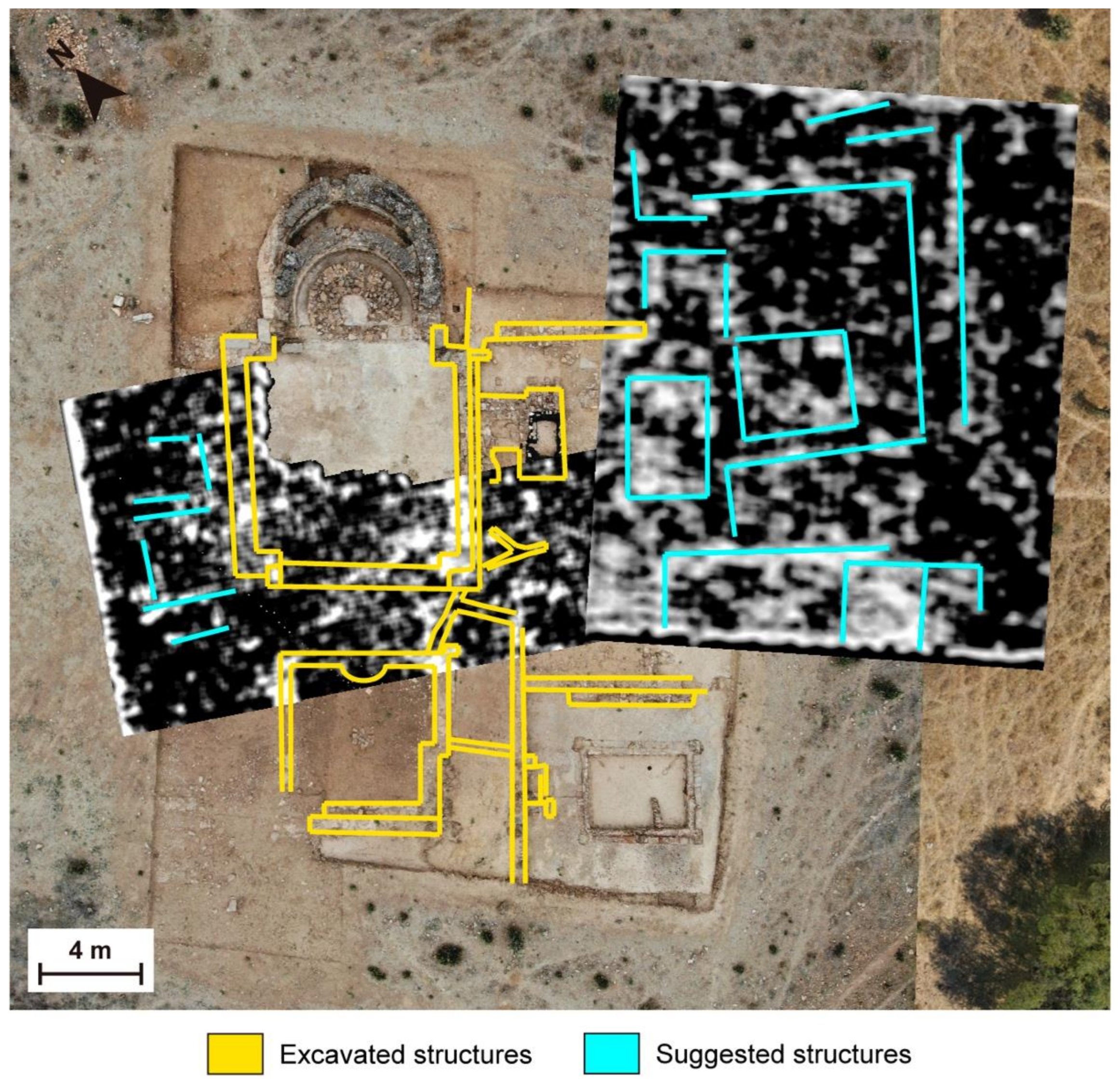
1.2. Archaeological Site: The Roman Villa of Horta da Torre (Fronteira, Portugal)

The design of the proposed methodology used GPR datasets with high density and quality acquired at the Roman villa of Horta da Torre, located in Fronteira municipality (Alentejo, Portugal) (Figure 1a). This archaeological site is part of the former Roman province of Lusitania. There are other villae examples in the surroundings with similar monumental pars urbanae surrounded by buildings for agricultural operations [3].

Horta da Torre is an excellent example of an opulent classical villa (Figure 1b,c), with good construction, high monumentality, and high-quality structural elements. The building is on a gentle slope, facing south and west, with excellent visibility, plenty of water resources, great pedological variety, and its diverticulum. It is approximately 500 m from the XIV route, a principal Antonine route between Olisipo (Lisboa, Portugal) and Augusta Emerita (Mérida, Spain).

Until 2012, we knew only three structural cores: the Bath, a 15 × 25 m tank with an opus signinum covering, which has two partially preserved walls and a third tomb; the Tower, an excellent apse structure that was interpreted as a part of a thermal building or to the pars urbana of the villa; and the Mosque, a mosaic-covered apse, far from the central nucleus. Approximately 30 m south of Bath, we identified extensive floors of opus signinum.

After 2012, the excavations revealed the existence of structures such as walls and pavements (Figure 2). Close to the apse structure, a stibadium was discovered, located at the back of a richly decorated room and covered by large slabs of white marble. Only remains were discovered at the bottom. These would be covered with opus tesselatum on the walls or ceiling according to many traces of fragmented mosaics found in an inverted position in the layer of sediment that covers the space of the room. The excavation reveals that the stibadium crowned a room with running water throughout the floor, released by a hatch hidden in the apse behind the stibadium. This floor had a robust and high-quality opus signinum floor with a half-round around the baseboard connected to the marble slabs. Next to this room, there is a large perystilium. At the base of the columns is a wall with a water pipe inside. There is also a smaller perystilium, suggesting that it may have a more personal character than the other structures.

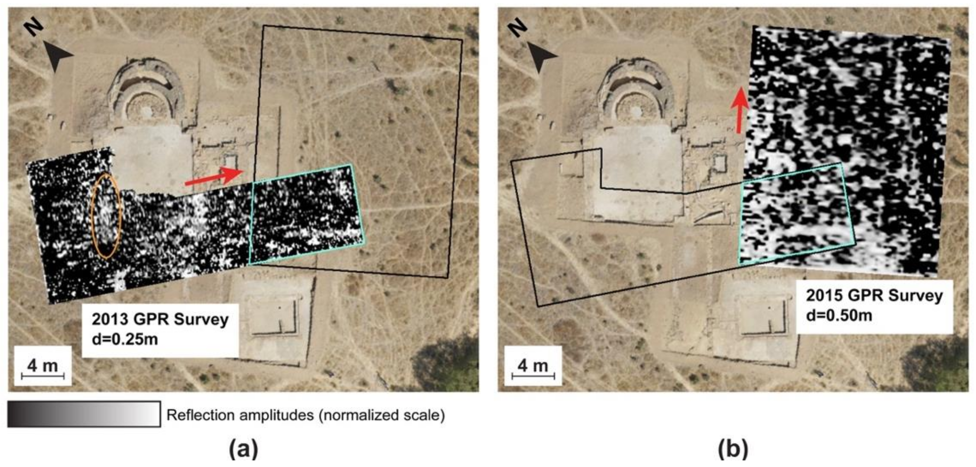
1.3. GPR Surveys Performed in the Site

Around the double apse structure, two GPR survey areas were defined (Figure 1b). The first survey, carried out in 2013, was performed with a B-scan spacing of 0.25 m. Because a portion of this space lies on an excavated section of the site, it has an uneven shape. The B-scans have a maximum length of 31.0 m, acquired in a width of 14.5 m. The survey execution time was approximately 4 h. The second survey, carried out in 2015, was performed with a B-scan spacing of 0.50 m. Obstacles such as dense bushes and stones contributed to the increase in the distance between the B-scans compared to the previous study. As a result, this area has a regular shape, with dimensions of 19.0 m and 22.9 m. The survey execution time was approximately 2 h. Both surveys were performed with GSSI SIR-3000 equipment, using a 400 MHz antenna.

Table 1. Acquisition parameters of GPR surveys.

Acquisition Parameters	2013 Survey	2015 Survey
Antenna frequency (MHz)	400	400
Number of B-scans	59	39
Distance between B-scans (m)	0.25	0.50
Antenna frequency (MHz)	400	400
Scans per meter	50	40
Samples per trace	1024	1024
Temporal depth (ns)	100	50
IIR band-pass filter (MHz)	100–800	100–800

lists the configuration parameters for both acquisitions.

The GPR datasets had a standard processing flow that allowed the best interpretation of the buried structures at the site (detailed in

Table 2. Processing parameters of GPR datasets, performed in the GSSI RADAN software.

Processing Operation	2013 Survey	2015 Survey
Correction of the surface position	5.37 ns
IIR filters	11 traces	13 traces
Gain adjustment	Constant in time window
Kirchhoff migration	Width 11; velocity 0.04 m/ns
Predictive deconvolution	N = 17; Predictive lag = 3
FIR filters	295–580 MHz
Gain adjustment	Linear, 7 points
Hilbert transform	Magnitude

). It includes the correction of the surface position, infinite impulse response (IRR) filters, constant gain adjustment, migration, deconvolution, finite impulse response (FIR) filters, linear gain adjustment, and Hilbert transform. GSSI RADAN 6.5 is the software used to implement this processing sequence. The last operation consisted of generating a 3D volume, often referred to as the 2.5D model, from which depth slices at several depths with the same thickness were extracted. Finally, from all depth slices, the cover surfaces [4] of both datasets were calculated and overlapped to an aerial orthophoto (Figure 3). In the cover surface calculation, from each depth slice, the reflections with a greater expression were estimated by comparison with the background amplitude value of each depth slice. If this expressive range exists in the other depth slices, then the information is highlighted at several depth values so that its representation could provide a three-dimensional perspective of the reflection alignments.

The value of 0.04 m/ns for the velocity was measured experimentally by modeling the hyperbola shape in the migration parametrization step. This value is compatible with the expected value reported in the literature for organic soil, such as Horta da Torre soil.

The 2013 results show alignments of reflections compatible with walls and pavements (Figure 3a). The survey carried out before the archaeological excavation guides the archaeologist to locations with a greater potential for the existence of buried structures. The excavation proved that the large reflectors correspond to a wall and pavement (Figure 2a). Further excavations confirmed that this was the corridor of the east wing of the main perystilium. The 2015 results (Figure 3b) also show alignments of reflections, but with less definition and sharpness comparing to the previous survey.

These results highlighted an important aspect: the characteristics of the wall of the Figure 2a, its large size, robustness, and excellent condition, are not noticeable in the GPR results. The data show that the structure exists, but they cannot report its large size.

Although the GPR results show reflectors, suggesting buried structures at the site along the data processing chain, there are some issues related to data density. The data are dense with the B-scan direction, as they have a sampling rate of 40 to 50 traces per meter, which gives a distance between traces of 0.025 m and 0.020 m, respectively. Perpendicular to the B-scan direction, each one is spaced 0.25 m in the 2013 survey and 0.50 m in the 2015 survey. Even if the distance between the B-scans is small, there is always a data imbalance in both directions. This question suggests that the data density can be a feature to consider. For example, a regular square mesh could be used during the acquisition step to avoid this transit effect of the antennas on the ground. On the other hand, the proposed approach makes it possible to increase the amount of data and information from the initial data.

2. Densification of 3D-GPR Data with Fourier Interpolation

2.1. General Overview of Trace Generation

A lateral data densification strategy is proposed as a complementary operation to standard processing. The methodology consists of the interpolation of GPR B-scans in the spectral domain after applying the Fourier transform. This mitigates the subsampling problem of 3D-GPR models. This method is widely used in seismic processing, allowing the estimation of missing traces from existing traces [5,6,7,8,9,10,11].

The first aspect to consider, to densify a 3D-GPR dataset, is that the type of information available corresponds to a spatial distribution of amplitudes, $A\left(x_i,y_j,z_k\right)$, resulting from the detection of reflected EMW. However, this dataset is not equally distributed in space since $A\left(z_{k=1:N_k}\right)$ represents a trace where $N_k$ corresponds to the number of samples, which generally has a value of 512 or 1024 samples, for spacing ($\Delta z$) between 0.05 and 0.5 ns. On the other hand, $A\left(x_{i=1:N_i}\right)$ denotes the amplitude of the signal received at each point of a depth along the B-scan, where $N_i$ denotes the number of traces in that B-scan; this defines the B-scan direction. This value depends on its length and the spacing between traces ($\Delta x$), usually between 1, 2, and 5 cm. Finally, $A\left(y_{j=1:N_j}\right)$ refers to the amplitudes when fixing a plane $\left(x,y\right)$ in which $N_j$ corresponds to the total number of B-scans acquired during the survey, with a certain spacing between B-scans ($\Delta y$).

When comparing the considered sampling intervals, it becomes evident that the dataset has subsampling in the y-direction, which results in a lack of information. Therefore, an excellent strategy to increase the quality of 3D images is to densify the whole set in this direction to generate new traces between the existing parallel B-scans.

2.2. Trace Estimation in Seismic Processing

For the estimation of traces from the existing traces, seismic exploration processing flows offer a variety of choices. One approach utilizes mathematical transformations (such as the Fourier and curvelet transforms) to estimate missing features in seismic data [5,12,13,14]. These transformations map the signal in a new domain to synthesize data in spatial locations that have not been recorded [5]. Other methods rely on using the Fourier transform [15,16,17,18,19]. Its coefficients are calculated from the input lines to estimate the data for any mesh dimension [20]. In addition, there are other proposed algorithms, such as the irregular Fourier transform and sparse inversion, which are efficient methods in the case of regularly sampled data. All Fourier reconstruction methods require two conditions: the signal must be limited over a range of frequencies and represented by a distribution of Fourier coefficients.

The use of mathematical transforms [8] and predictive filters [21] in the f-x domain [22] is one of the interpolation strategies for estimating missing traces in seismic data. We can perform the data estimation using predictive filters as autoregressive operators since linear events overlap in the f-x domain. We can also apply the method to f-x random noise attenuation phenomena [23,24,25]. For example, to interpolate data with a frequency of 2f, we can use predictive filters estimated from frequency f. Predictive filters estimated from low signal frequencies, free from aliasing, are used to interpolate the content of high frequencies that suffer from aliasing and can also be used to reconstruct missing data [22,26,27].

Automatic event identification is a technique that allows trace interpolation and the estimation of parameters or attributes [28,29]. We use the amplitudes corresponding to the reflections and arrival timings [30]. The algorithm analyzes the attributes of the recorded datasets [30,31,32] and converts the signal into reflection amplitudes and the cosine of the instantaneous phase. The algorithm uses the phase cosine to identify any event with lateral continuity of the phase value, connecting phases of the signal with the same polarities and close arrival times [29]. Reflection impedance allows the system to identify events in which there is a lateral variation in amplitudes or changes in the configuration of the reflected wave. The algorithm automatically connects events that have lateral coherence, defining horizons, which are then analyzed by overlapping them with the initial seismic profile. The analysis of each horizon seeks nearby subparallel events to classify them as part of the exact reflection. When grouping events, it is possible to estimate the reflection points by calculating the mean cosine of the phase of each horizon, preserving the reflected signal, and removing unrelated events [29].

We can apply automatic event identification to calculate spatial derivatives after applying the Fourier transform. Analogous to temporal derivatives, spatial derivatives also convert inflection points into zeros (in spatial terms), allowing any special discontinuity of seismic data to be highlighted [33]. In addition, we can also apply spectral analysis to spatial derivatives, which denotes that differentiation in the horizontal direction increases the frequency content and applies a phase shift of π/2. As a result, we may employ derivatives to detect small changes in the seismic signal caused by interfaces such as meshes and cracks [33].

Referring to the classical interpolation method, spatial interpolation can also be used in the B-scan and depth slice. Whichever grid method is used, the interpolation is performed through the analysis of neighboring pixels. Even with the great efficiency that applies most of the time, in certain situations, numerical artifacts are generated, an event that we aim to avoid.

The choice of Fourier interpolation is because this scheme maintains the spectral content of the data. The reason for the preference for B-scan interpolation considering 2D rather than 3D interpolation is that the acquisition of GPR B-scans is performed through 2D parallel B-scans. As the interpolation is performed at the trace level, it is not relevant to compare this interpolation scheme with others.

It is also necessary to say that a GPR B-scan, in the frequency domain, is limited by a range of values and must be able to be represented by a distribution of Fourier coefficients. These two conditions were previously verified in [34,35].

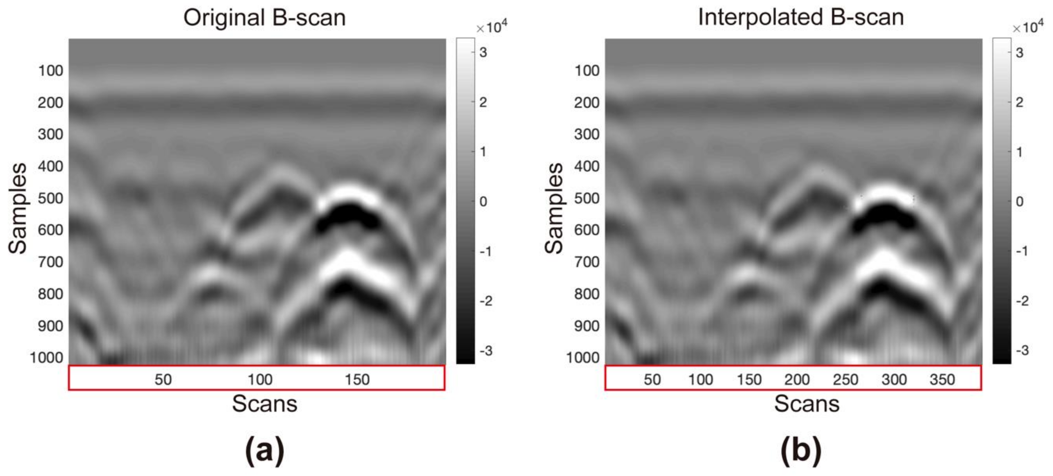
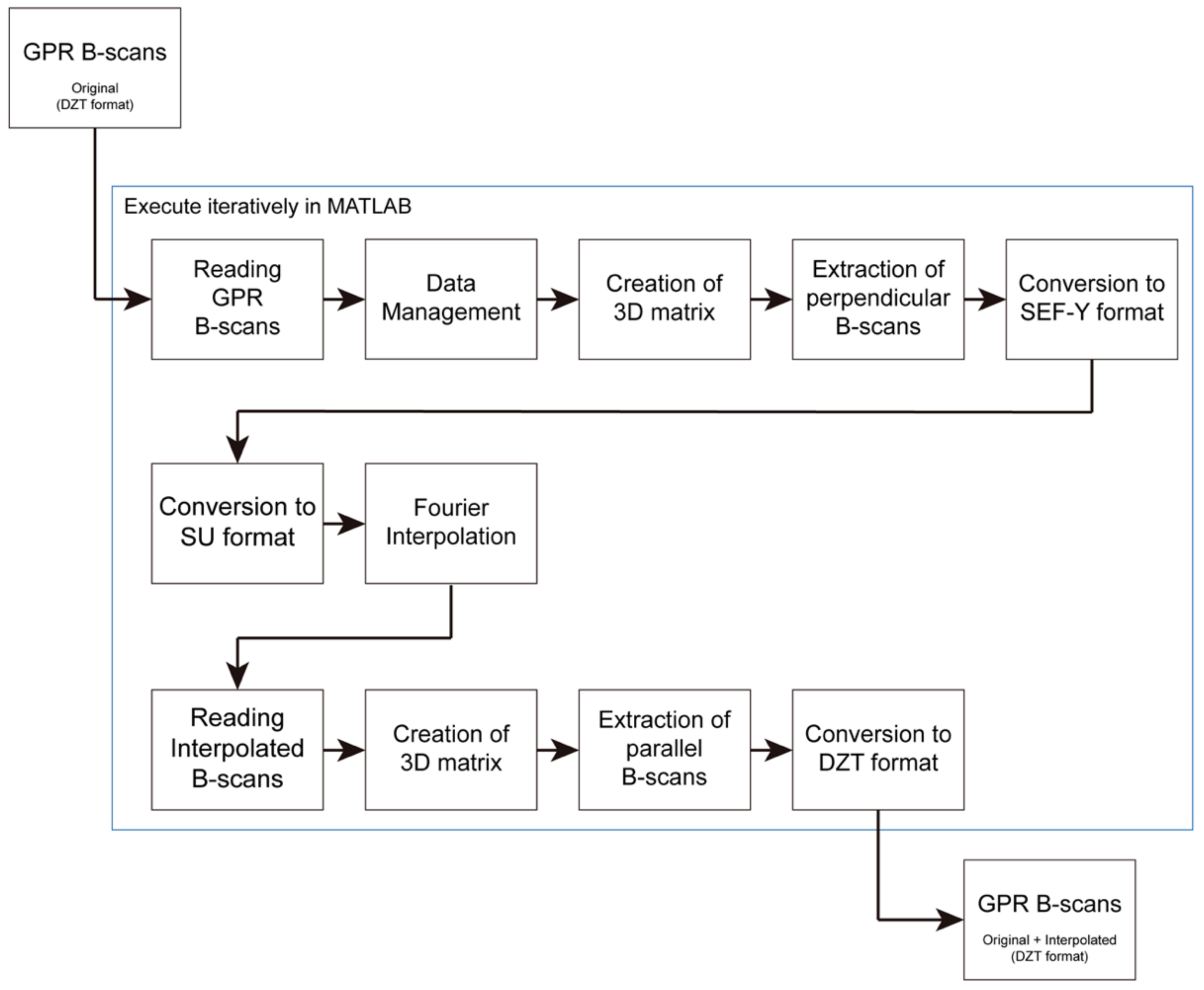
2.3. INT-FFT Algorithm to Interpolate GPR B-Scans

This study used the Fourier interpolation method to generate traces and densify the dataset in the frequency domain. The implementation is made through the Suinterp algorithm [36,37], available in Seismic Unix (SU), a free access utility package from the Centre for Wave Phenomena of Colorado School of Mines (USA). This algorithm interpolates traces between each pair of existing traces by applying the discrete Fourier transform to each trace and calculating the spatial derivatives of each pair of adjacent traces. Then, it performs a linear interpolation between both traces in the frequency domain and applies the inverse of the Fourier transform, restoring the data to the time domain. We assume that the low-frequency content of the input signal does not suffer from aliasing and that the deeper amplitude peaks allow data interpolation across its entire bandwidth at the high frequencies that are subsampled.

The parameterization of the algorithm contains the number of lines to be interpolated between each pair of lines, the total number of traces in the B-scan, and corner frequency values corresponding to the GPR data frequency range.

Before applying the methodology to the entire 3D-GPR dataset, it is necessary to test with a GPR B-scan to compare the input with the output using a B-scan acquired in a laboratory with a 1.6 GHz antenna. The acquisition parameters are as follows: 1024 samples per trace, 5 ns temporal range, 0.004888 ns sampling interval, 196 samples per trace, and 0.005 m equidistance of traces. The interpolated B-scan must have 391 traces, twice the traces minus one (proven information, Figure 4). The time range remains the same, and the distance between the traces decreases to half of the initial value before interpolation, to 0.0025 m.

Figure 4 shows the input and interpolated B-scans. There is a slight increase in sharpness after implementing Fourier interpolation with the Suinterp algorithm. We also did not notice any change in the range of amplitude values. The quality of the initial data has not decreased. We can conclude that this interpolation method works for GPR data.

MATLAB was used to create the previous tests and the script. The Suinterp algorithm requires converting the GPR data to a compatible format. The adaptation of the data implies the manipulation of the matrices so that they are spatially related and so the desired information can perform the interpolation, and then the export of the matrices to the format allowed for import by the Suinterp algorithm.

As the data were acquired in N equally spaced parallel lines, the import of all B-scans needs to store the data in the form of a 3D matrix, A(x_i, y_j, z_k), corresponding to the spatial distribution of the lines (Figure 5a). The 3D matrix has dimensions (N_i, N_j, N_k) in which N_i and N_j are each row and column of each B-scan, respectively, and z_k defines the sample number of the line corresponding to the pair (x_i, y_i).

To densify between the B-scans, first, it is necessary to redefine B-scans in the y-direction, meaning that the B-scans to be considered are perpendicular to the initial direction (Figure 5b). Each redefined B-scan consists of a trace from each original B-scan, sequentially ordered from j = 1 to N_j. This data rearrangement is necessary because the Suinterp algorithm interpolates a trace between each pair of traces. As a result, we need to apply the parallel B-scan interpolation as many times as the number of traces in the perpendicular B-scan. The next step is to restore the original direction of the spatial reference, redefining the B-scans along the x-direction, as in the original data (Figure 5c). In total, the number of final B-scans is 2N − 1.

The entire sequence of operations is applied iteratively, which allows one to automate the entire procedure. The user must compile the algorithm and wait for the result.

The following process sequence (Figure 6) is the flow scheme to implement the densification technique in the MATLAB software:

• Preliminary parameterization: introduction of the total number of parallel B-scans and the number of the initial B-scan.
• Importing GPR B-scans in DZT format using routine readgssi, a MATLAB algorithm adapted to read files in DZT format.
• Determination of the maximum length of the B-scans so that the 3D matrix is regular.
• Importing complementary information about the geometry of the dataset (starting and ending position of each B-scan); all B-scans must be well located in space. During the survey, the user needs to collect all the information about the acquisition.
• Determination of the extremes of the locations of each B-scan.
• Removal of the effect of the acquisition in zigzag, if necessary.
• Normalization of the length of the B-scans, if necessary, by adding traces of zeros at the start or end of the B-scan to make the matrix regular.
• Placing the data for each B-scan in the 3D matrix (parallel B-scans).
• Extraction of perpendicular B-scans and conversion to SEG-Y format using the routine MATLAB writesegy (SegyMat Library).
• Conversion to SU format using internal Seismic Unix routines.
• B-scan interpolation using the Seismic Unix Suinterp routine.
• Importing interpolated B-scans in SU format using the MATLAB readsu routine (SegyMat Library).
• Placing the interpolated data in the 3D matrix.
• Extraction of parallel B-scans (original + interpolated).
• Data conversion to DZT format, using the MATLAB writegssi routine, developed to write files in DZT format.

Figure 6. Schematics of the numerical implementation of the INT-FFT algorithm.

Figure 6. Schematics of the numerical implementation of the INT-FFT algorithm.

2.4. Parameters to Evaluate the Results

The evaluation of the results of this methodology is made by establishing a comparison between the different datasets graphically and by the values of parameters such as the structural similarity index and sharpness index.

The structural similarity index (SSI) quantifies the similarity between two datasets [37]. The result can be represented graphically (displayed differences) and as a percentage (100% corresponds to the same data).

The sharpness index (SI) is a parameter that quantifies the sharpness of an image with dimensions (mxn). To calculate it, we can use the Hudgin gradient (dH) of the image [38]; it is used in image fusion to select the sharpest pixels [39] considering the neighboring pixels. The numerical implementation requires calculating the horizontal components of the Hudgin gradient dxH and vertical dyH. These coefficients are needed to calculate the gradient modulus used in the SI calculation [40] through Equation (1).

$$Sharpness index=100\ast {{\displaystyle \sum }}_{i,j}^{m,n}\frac{{{\displaystyle \sum }}_{i,j}^{m,n}\left|d{H}_{i,j}\right|}{m\times n}$$

(1)

where $m\times n$ is the dimension of the matrix and where i,j defines the coordinates of each cell.

The Hudgin gradient values of the image increase with increasing image contrast. We can consider that the sharpness of an image must be associated with the diversity of contrasts: the more significant and more abundant the contrasts are, the greater this index.

Both parameters are a way to quantify the improvement that Fourier interpolation can provide to the results. It should be noted that data densification increases noise levels, so the sharpness index must be analyzed carefully.

3. Results

3.1. 2013 GPR Dataset

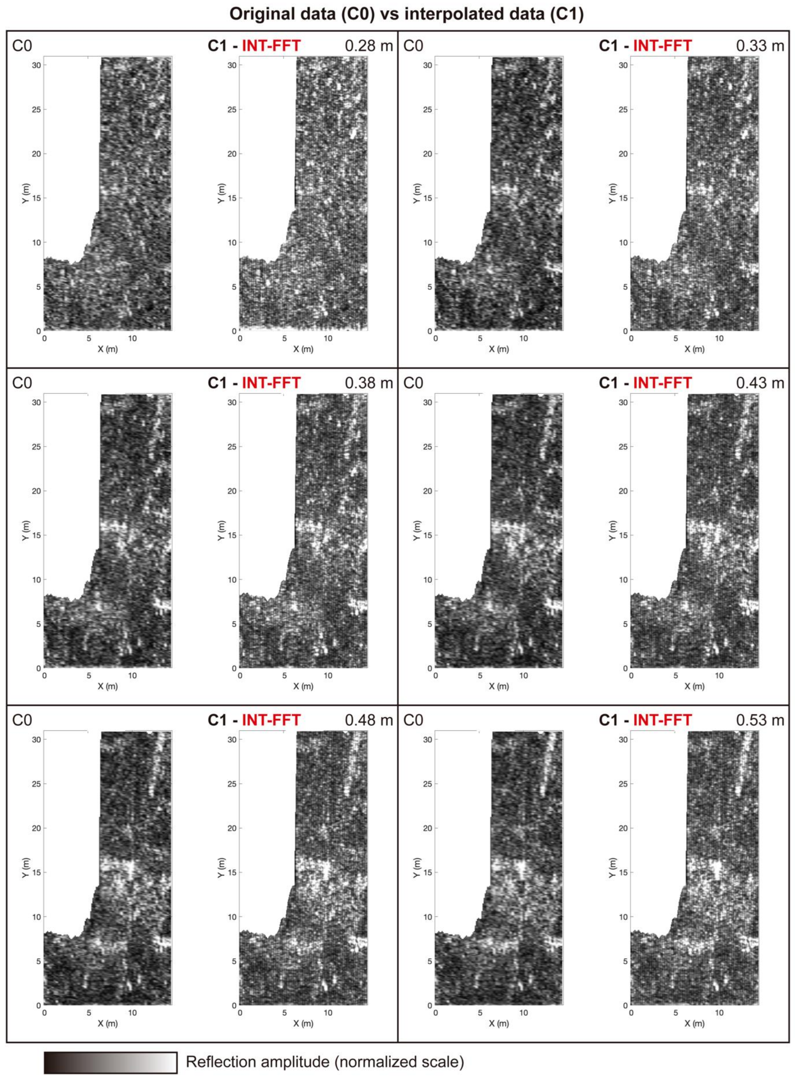
The original dataset (without processing) was used as an input in the INT-FFT algorithm to produce the interpolated dataset. We applied standard processing flow to both datasets, with the necessary changes to the new one due to the reduced B-scan spacing (correction of the surface position, IIR filtering, constant gain adjustment, Kirchhoff migration, predictive deconvolution, FIR filtering, linear gain adjustment and Hilbert transform). The approach was the same as previously described. Some tests were necessary to evaluate it.

Therefore, the pairs of datasets to consider for method analysis are the following:

(1)

Original data, C0 (d = 0.250 m) versus interpolated data, C1 (d = 0.125 m): To assess the effects of Fourier interpolation on the lateral densification of GPR B-scans.

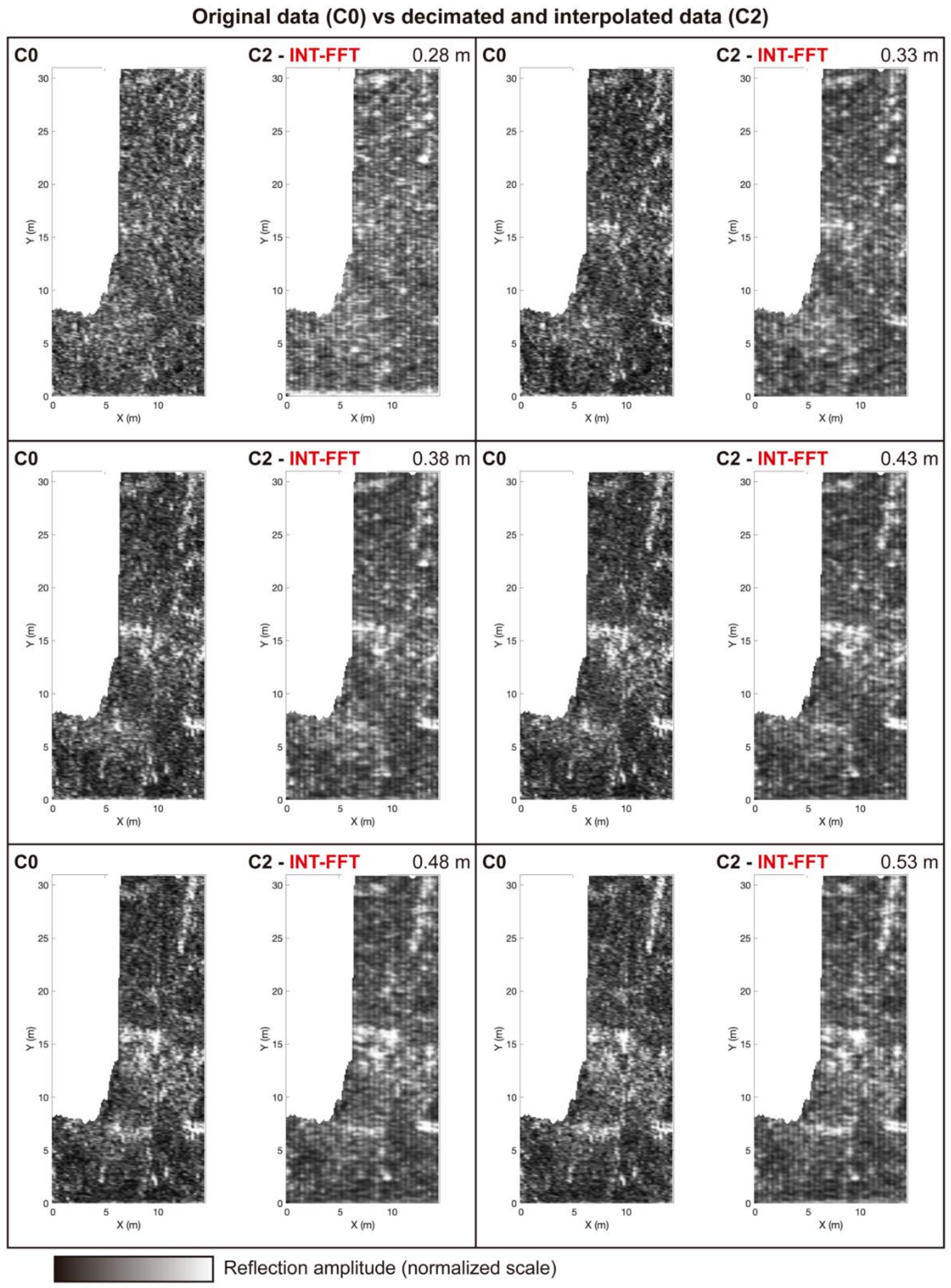
(2)

Original data, C0 (d = 0.250 m) versus decimated and interpolated data, C2 (d = 0.250 m): To assess the level of missing information estimated through Fourier interpolation; for this, we need to decimate the original data with the elimination of B-scans interspersed (between every three, we erase one in the middle) to make the spacing between B-scans at d = 0.500 m; the interpolation resets the original spacing between B-scans (d = 0.250 m).

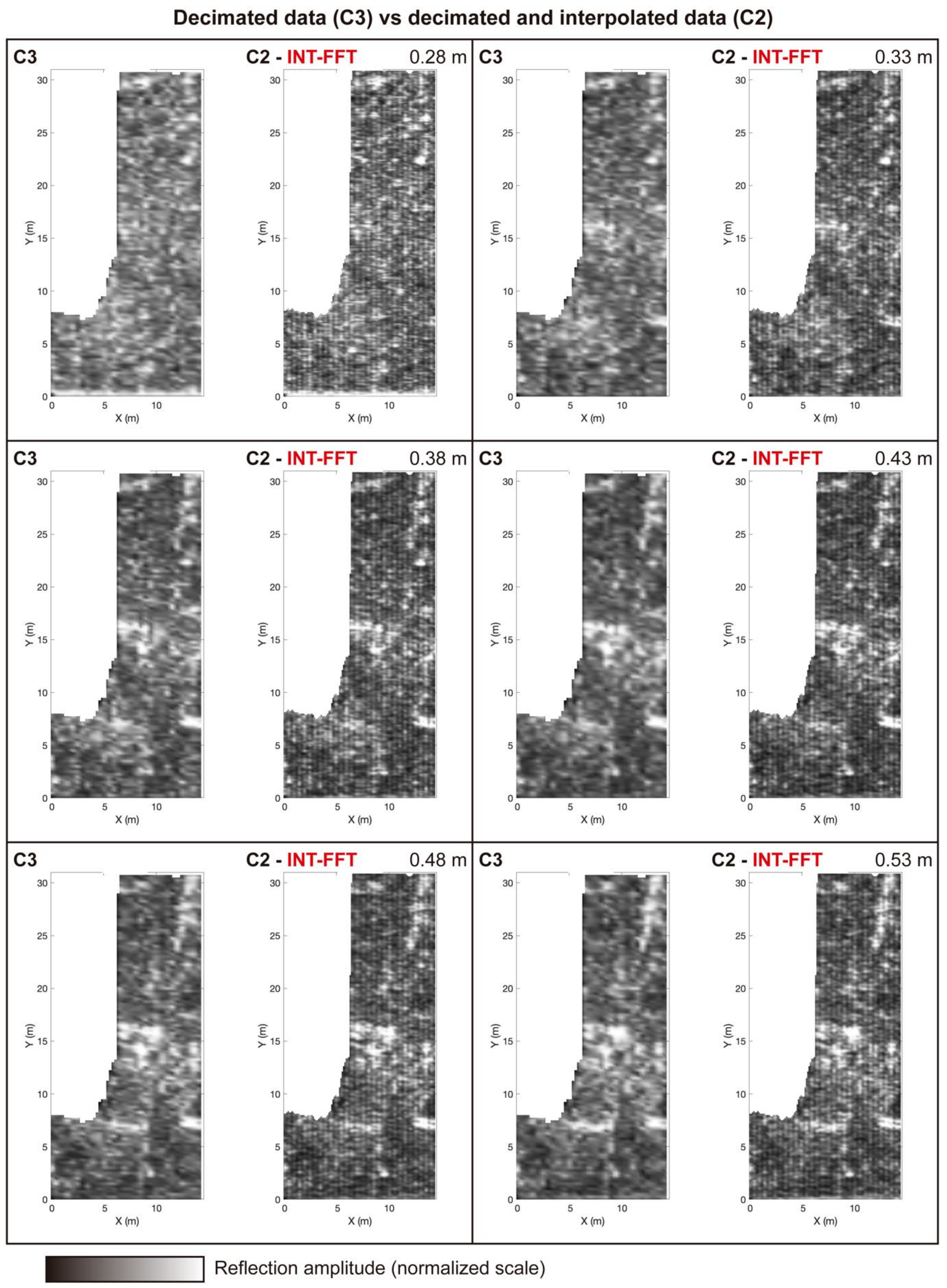
(3)

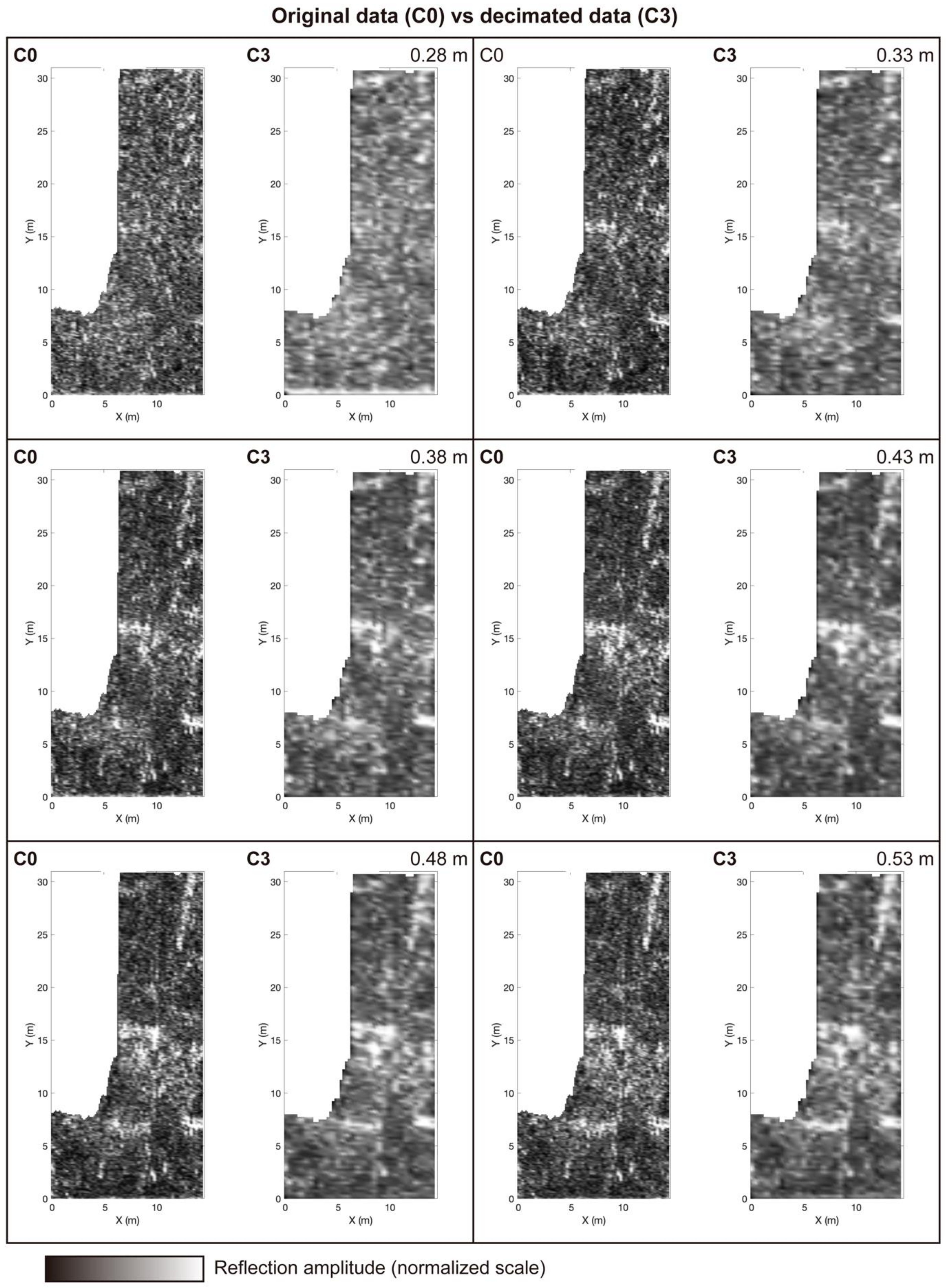
Original data, C0 (d = 0.250 m) versus decimated data, C3 (d = 0.500 m): To assess what information is lost when we choose to increase the spacing between the B-scans to make the survey faster, which may allow increasing the prospected area.

3.1.1. Original Data (d = 0.250 m)—Default Dataset—C0

The original dataset, C0, was acquired in parallel B-scans spaced at 0.250 m. The processing flow applied is the same as described in Section 1.3. After that, we extract depth slices from the 3D model. The considered depths are the following: 0.28, 0.33, 0.38, 0.43, 0.48, and 0.53 m. The integration thickness of all slices is the same: 0.11 m.

The depth slices between 0.33 m and 0.53 m show alignments compatible with wall-type structures. The archaeological excavation proved the existence of the walls. However, despite the alignments being quite evident in their correspondence to buried structures, there is some difficulty in individualizing these alignments at some depths. This may be due to the collapse of these structures, causing additional reflections and the B-scan spacing. Nevertheless, these results are considered standard and used for comparison with other datasets.

The comparison of results was carried out through direct observation and by analyzing the values of the structural similarity index (

Table 3. Structural similarity index between different datasets at different depth slices.

Depth (m)	Structural Similarity Index (%)
	C0 VS. C1	C0 VS. C2	C0 VS. C3
0.28	81.17	62.49	62.78
0.33	82.50	63.02	62.62
0.38	82.44	64.98	65.49
0.43	82.65	64.16	65.23
0.48	82.66	65.10	65.47
0.53	82.62	65.17	66.87
Mean	82.34	64.15	64.74

). We also calculated the average sharpness index for each set of images, which in the original data presents an average value of 11.44% (

Table 4. Sharpness index between different datasets at different depth slices.

Depth (m)	Sharpness Index (%)
	C0	C1	C2	C3
0.28	13.14	17.80	12.30	9.88
0.33	12.13	15.79	11.09	8.99
0.38	11.22	14.96	10.47	8.51
0.43	10.64	14.23	9.83	7.99
0.48	10.93	14.43	10.08	8.18
0.53	10.60	14.60	10.28	8.25
Mean	11.44	15.30	10.68	8.63

).

3.1.2. Interpolated Data (d = 0.125 m)—C1

The interpolated dataset, C1, was obtained from C0 by applying the INT-FFT algorithm. The original data spacing of 0.250 m then changed to 0.125 m, half the initial distance.

The effectiveness of the algorithm was graphically evaluated (Figure 7) by comparing the depth slices extracted from the C1 and C0 datasets. Although there was no production of numerical artifacts originating from the interpolation process, the reflection alignments generally seemed better defined and sharper in C1 depth slices than in C0. More minor alignments, which appeared less sharp in the initial data, showed the most improvement. They became more individualized and more perceptible. The other alignments were initially quite clear, and there was an increase in their definition.

The structural similarity index (Table 3) presented an average value of 82.34%. The two datasets were similar, and the interpolation did not change. The average sharpness index is 15.30% (Table 4). There was an increase in sharpness between the interpolated and original data (+3.86%).

3.1.3. Decimated and Interpolated Data (d = 0.250 m)—C2

The decimation of the original data aims to examine the extent of data estimation with this interpolation approach. First, we delete the middle B-scan, resulting in a shift in the distance between B-scans from d = 0.250 m to d = 0.500 m. Subsequently, we apply the INT-FFT algorithm to make the distance between the B-scans equal to the initial distance (d = 0.250 m) again. Figure 8 shows the graphical comparison between the C2 and C0 datasets.

As in the previous case, we do not note the production of numerical artifacts, and the interpolation allowed the estimation of missing information. However, it is impossible to estimate all the expected information, as highlighted by the reduced definition and sharpness of the initially observed reflection alignments. The average value of the structural similarity index (Table 3) decreased to 64.15% (−18.19%). Similarly, the average sharpness index decreased (−0.76%) to 10.68% (Table 4).

3.1.4. Decimated Data (d = 0.500 m)—C3

Finally, we establish a comparison between the original and decimated data (Figure 9) to assess the level of information lost when the spacing between B-scans increases. We compare the results from C0 (d = 0.250 m) with those produced with decimated data from the previous case (d = 0.500 m), C3. The graphical analysis of decimated data allows us to verify that the definition of the reflection alignments observed in C0 has considerably decreased. However, it is still possible to distinguish the more robust alignments. The mean value of the structural similarity index (Table 3) decreased to 64.74% (−17.60%).

It is essential to highlight a detail verified after the graphical analysis between the decimated data, C3, and the decimated and interpolated data, C2 (Figure 10). The INT-FFT algorithm can correctly estimate some information that is not present in the decimated data. For example, the average sharpness index of C3 is 8.63% (Table 4), which is lower than the value observed in C0 (−2.81%).

The next step is the production of cover surfaces from the C0 and C1 datasets (Figure 11). This step considers only the depth slices between 0.38 m and 0.53 m. When we select all the depth slices together, the cover surface exhibits information gaps due to slices with less information. As a result, the user must choose slices carefully. The C1 dataset shows an increase in reflection alignments corresponding to wall-type structures. There is also an increase in background reflections that appear to be noise. The sharpness index for both datasets increased from 13.37% to 26.19% (

Table 5. Sharpness index of the cover surfaces from 2013 GPR datasets before and after INT-FFT processing. The sharpness increases with additional applied processing.

GPR Dataset	Sharpness Index (%)
	Standard	INT-FFT
2013	13.37	26.19

).

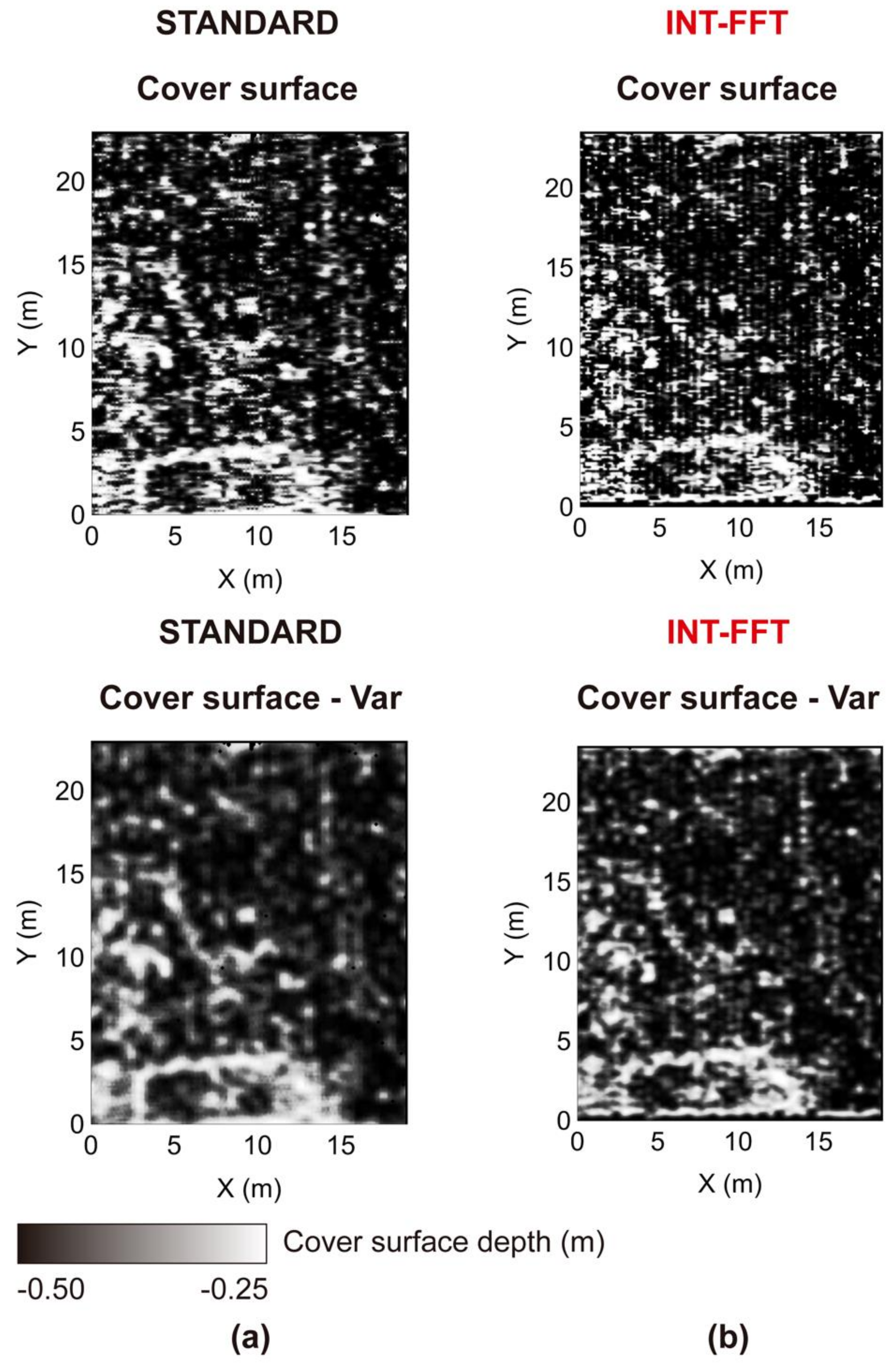
3.2. GPR 2015 Dataset

Another GPR dataset, gathered in 2015, was likewise subjected to the proposed technique. The distance between the B-scans is 0.50 m, which is higher than that in the 2013 dataset (0.25 m). The results obtained from a standard processing flow (correction of the surface position, IIR filtering, constant gain adjustment, Kirchhoff migration, predictive deconvolution, FIR filtering, linear gain adjustment and Hilbert transform) displayed in Figure 12 show reflection alignments that can correspond to buried walls. The main characteristic observed is that the alignments are not as sharp as in the 2013 dataset. Applying the INT-FFT algorithm to reduce the B-scan spacing from 0.50 m to 0.25 m, the results for each depth slice reveal an increase in data density, which indicates an increase in the sharpness of the reflection alignments.

The next step is the production of cover surfaces from the standard and interpolated datasets (Figure 13). Both datasets show vertical stripes in the same direction as the B-scans. The sharpness index for both datasets increased from 21.03% to 27.19% (

Table 6. Sharpness index of the cover surfaces from 2015 GPR datasets before and after INT-FFT processing. The sharpness increases with additional applied processing.

GPR Dataset	Sharpness Index (%)
	Standard	INT-FFT
2015	21.03	27.19

).

Due to the acquisition characteristics, such as soil grooves or dense vegetation, depth slices and cover surfaces can present vertical stripes with the parallel direction of the B-scans. We can suppress this effect by applying a directional filter to the depth slices and cover surfaces, increasing the coherence of the signal.

We can compute this in the software Golden Surfer by calculating the experimental semivariogram to use it in the gridding operation [41]. This procedure aims to obtain information about the distribution of values located around a mesh point. The experimental semivariogram represents the statistical trend of the spatially distributed values and can be fitted to an analytical curve and used in interpolation to generate a 2D mesh. We successfully tested this postprocessing on the GPR data [35], and its effectiveness is demonstrated in the 2015 GPR dataset.

3.3. Interpretation of Geophysical Results in the Scope of the Archaeological Site

After densifying the GPR datasets through the INT-FFT algorithm, it is possible to update the previous interpretation in an archaeological context by overlaying the processed cover surfaces to an aerial image obtained by an unmanned aerial vehicle (Figure 14). Yellow lines indicate structures discovered after excavation. In blue are the reflection alignments that suggest that they are wall-type buried structures.

This type of output allows us to observe that the alignments of reflections resulting from the GPR surveys correspond to the structures excavated later. Similarly, the remaining alignments in the unexcavated sites are consistent with the other structures. The results also show some evidence of a slight rotation in some preferred directions.

4. Discussion of the Results

The results obtained after implementing the INT-FFT algorithm show that the proposed approach effectively increased the lateral resolution of the 3D-GPR datasets. Data densification through 2D Fourier interpolation allowed the creation of a new GPR B-scan between each pair of existent B-scans. This approach increased the general sharpness of the obtained GPR results.

The numerical implementation started with a test in a single B-scan to ascertain the applicability of the Suinterp algorithm to GPR data. The graphical aspect remained, with a change in the number of traces that increased from N to 2N − 1. In addition, we observed a slight increase in the sharpness of some reflectors. Therefore, the INT-FFT algorithm could densify the GPR data, and we could use it to interpolate the B-scans in a 3D dataset.

We created the algorithm based on the 2013 GPR data from the Roman villa of Horta da Torre. The survey with parallel B-scans spaced 0.25 m apart had an irregularly shaped area. The short distance between the B-scans gave the survey a high-density character, which increased the quality of the results. We performed several tests to determine the impact of data densification using this method. The evaluation of the results was performed by graphical analysis of depth slices at several depths and by calculating parameters such as the structural similarity index and sharpness index.

The first test aimed to study the efficiency of the proposed interpolation scheme by comparing the original data (C0) and the interpolated data (C1) after applying the standard processing flow to each one. The analysis of depth slices at several depths showed that the alignments of reflections became more defined and without the numerical artifacts produced by the interpolation. The mean value of the structural similarity index of this pair of results was 82.34%. The two datasets had similar characteristics, which were consistent with the depth slice analysis. The sharpness index increased from 11.44% (C0) to 15.30% (C1). We also note that the interpolated dataset showed an increase in brightness. This effect was related to the dispersion created by collapses. The interpolation of the B-scans estimated the signal corresponding to buried structures and the surrounding environment. It was not possible to prevent this from happening; however, we knew that it was possible to eliminate this effect by applying filters dedicated to noise removal.

The second test aimed to assess the missing information estimated after the data decimation, followed by interpolation by comparing the original data (C0) and the decimated and interpolated data (C2). Fourier interpolation allowed us to estimate the missing data. However, it could not replace these data in full. When the distance between the B-scans was too large, the antenna footprint of the side data was not able to detect the information in the location of the data to be interpolated. Therefore, graphically, we observed a decrease in the definition of some reflector alignments. The average value of the structural similarity index decreased to 64.15%. Both datasets were similar, but interpolation failed to estimate the part of the missing information in the original decimated B-scans without significant expression in the adjacent B-scans kept. The estimation efficiency depended greatly on the object size. Objects smaller than the spacing between the B-scans could hardly be estimated. The average sharpness index of the decimated and interpolated data (C2) decreased to 10.68%.

The third test evaluated the level of information lost when the spacing between the B-scans increased by comparing the results produced with the original data (C0) and those made with the decimated data (C3). The structural similarity index had an average value of 64.74%, identical to the previous comparison. We interpreted that the densification of very spaced B-scans could not estimate the missing data. However, the amount of information contained in the decimated dataset, compared to the original dataset, decreased considerably, especially the definition of the reflection alignments present in C0. The sharpness index for an average value fell to 8.63%. However, in the C3 case, the reflection alignments allowed the identification of alignments of reflections compatible with wall-type structures.

The fourth test compared the decimated data (C3) and the decimated and interpolated data (C2). The proposed interpolation method could estimate some missing information from the information contained in the existing B-scans. However, it could not estimate data when adjacent traces do not have lateral details. Therefore, the methodology may allow the sacrifice of the density of data acquired in the field. Nevertheless, it could be estimated in the processing step using the present interpolation technique applied in the frequency domain. However, this applies only under conditions where the objects to be detected have dimensions that allow them to be detected by adjacent B-scans. In addition, the increase in B-scan spacing may cause under-sampling that cannot be solved.

After applying the processing flow, we performed a final test on the 2013 GPR dataset by calculating the cover surfaces of the C0 and C1 datasets. Graphically, the C1 data became sharper than the existing reflection alignments. The value of the sharpness index increased from 13.37% to 26.19%. The cover surface showed that there was an increase in reflection alignments in the densified data. The brightness also increased, caused by the dispersions in the collapses. Overall, the result of the methodology in this dataset was better than the previous one.

We also tested the INT-FFT algorithm on the GPR 2015 dataset obtained from the same archaeological site, with a B-scan spacing of 0.50 m. The results after standard processing flow showed reflection alignments that suggested the existence of buried structures of wall type, such as the 2013 dataset. However, the high spacing between the B-scans decreased the sharpness of the reflection alignments compared to the dense dataset. After applying the interpolation, the results showed an increase in the data density, making them sharper. The improvement was more accessible to understand by analyzing the cover surfaces obtained before and after the interpolation. The increase in the values of the sharpness index, from 21.03% to 27.19%, also supported this improvement. In these data, we also observed a striped effect in the direction of the B-scans (vertical). Using a directional filter to correct this effect allowed its elimination, improving the data.

The combination of GPR results and aerial orthophotos allowed us to increase the comprehension of the existence of buried structures at the site. In addition, it was possible to add interpretation schemes to highlight structures already excavated, and suggested structures only detected with GPR. Finally, this approach determined preferred directions that could help interpret the detected anomalies before proceeding with the excavation.

Despite the effectiveness of the approach, we noticed some limitations during the development of the method and the testing steps. Before the beginning of the interpolation process, the user must insert the locations of each B-scan. This step can be made by uploading a CSV file. However, the data input needs to be conducted by the user. This step implies a very well-defined knowledge of the geometry of data acquisition. Any failure of the geometric information promotes a lag of the interpolated B-scans that increases the striped effect on the interpolated outputs in the direction of the B-scans. This effect is not due to the Suinterp algorithm but to some misalignments of the B-scans, which, even with the utmost care, can occur, and maybe to the unevenness of the ground during the acquisition. This graphical effect can be successfully eliminated or reduced through a correction considering the semivariogram of the data. Another limitation is a possible slow implementation of the algorithm, even using robust hardware. The algorithm is optimized to implement the interpolation process iteratively with success. However, most of the algorithms consist of manipulating many data matrices. This process becomes slow even if the algorithm is optimized and requires the hardware to have enough memory for that much data to be loaded into memory at the same time.

Another limiting aspect refers to the parameters used to evaluate the interpolation methodology presented. Both are not the best parameters but are just a suggestion to analyze the data, different from what exists in standard software. The sharpness index is a measure that should be considered with caution since when estimating new GPR data, noise caused by the collapse of structures is also being interpolated. This effect is reflected in the increased brightness of the analyzed depth slices, as well as in the cover surface. However, the overall value of this index increases with the application of the methodology.

We also explored another aspect, determining the best processing step to implement B-scan interpolation. Its application was considered after completing the entire processing chain, although the results were not satisfactory. The best time to implement the INT-FFT algorithm is early with the raw data. This may be because the implemented interpolation is performed in the spectral domain, requiring that the frequency domain data have coherence. By applying some processing operations, such as filtering, the spectral content of the data changes.

The possible advantage of Fourier interpolation applied within each B-scan to increase the number of traces was also explored. This approach was successfully used in the GPR 2015 dataset along all B-scans, significantly improving the data obtained.

Considering all the aspects mentioned, we can verify that this interpolation scheme is effective in estimating profiles among the existing ones. We cannot say that this interpolation methodology is better than others since its application has a different premise from the others. Interpolation is applied to each trace, considering the adjacent traces. Spatial interpolation, performed in 2D, for example, in depth slices, is not capable of estimating information based on the spectral content of the data; it is performed at the pixel level, analyzing its neighborhood.

Regarding the use of this methodology to densify the GPR data and consequently increase the quality of the results, this improvement is expected to translate into a better understanding of reflection alignments that may correspond to buried structures. If the data are initially dense, this improvement will hardly be noticeable. In a scenario where the distance between B-scans is high but not too much to create under-sampling, densification will promote the sharpening of the results, and the user can be better guided to better interpret the results in the archaeological context.

The continuation of this study should focus on the complete automation of the iterative process, decreasing the user dependence, and optimizing the algorithm so that the computing time can be reduced.

5. Conclusions

This study provides a new methodology for performing a spectral interpolation of ground-penetrating radar (GPR) data. The densification method increases the lateral resolution of 3D-GPR datasets through 2D Fourier interpolation, creating GPR B-scans between two that already existed. In addition, this approach improves the sharpness of the obtained GPR models.

The INT-FFT algorithm was tested effectively in two GPR datasets from the Roman villa of Horta da Torre (Fronteira, Portugal). Both had distinct acquisition parameters, such as the distance between B-scans (0.25 and 0.50 m) and sample rating (50 and 40 traces/m). The results showed an increase in the geometric sharpness of the GPR reflectors and did not produce any numerical artifacts.

The tests performed to apply the methodology to GPR-3D data allowed us to assess the interpolation efficiency, the level of estimation of missing data, and the level of information lost when choosing to increase the distance between B-scans in the acquisition stage of the data.

The use of the GPR B-scan interpolation methodology in the frequency domain proved advantageous in GPR-3D data densification to increase data clarity. However, we should highlight that the method works only when the data are dense enough to detect the presence of objects buried in the subsurface. Furthermore, the technique cannot generate information that is not present in the input data, so if these are under-sampled, the method is not able to produce the missing data.

References

1. Vickers, R.S.; Dolphin, L.T. A Communication on archaeological radar experiment at Chaco Canyon, New Mexico. MASCA Newsl. 1975, 11, 6–8. [Google Scholar]
2. Conyers, L.B.; Goodman, D. Ground-Penetrating Radar: An Introduction for Archaeologists; AltaMira Press: Walnut Creek, CA, USA, 1997. [Google Scholar]
3. Carneiro, A. Humanitas Supplementum no. 3. In Lugares, Tempos e Pessoas: Povoamento Rural Romano No Alto Alentejo; Imprensa da Universidade de Coimbra: Coimbra, Portugal, 2014. [Google Scholar]
4. Peña, J.A.; Teixidó, T. Cover Surfaces As a New Technique for 3D Gpr Image Enhancement. Archaeological Applications. RNM104—Informes. Univ. Granada—Inst. Andal. Geofísica 2013, 1–10. [Google Scholar]
5. Liu, W.; Cao, S.; Li, G.; He, Y. Reconstruction of seismic data with missing traces based on local random sampling and curvelet transform. J. Appl. Geophys. 2015, 115, 129–139. [Google Scholar] [CrossRef]
6. Gülünay, N. Seismic trace interpolation in the Fourier transform domain. Geophysics 2003, 68, 355–369. [Google Scholar] [CrossRef]
7. Liu, B.; Sacchi, M.D. Minimum weighted norm interpolation of seismic records. Geophysics 2004, 69, 1560–1568. [Google Scholar] [CrossRef]
8. Spitz, S. Seismic trace interpolation in the FX domain. Geophysics 1991, 56, 785–794. [Google Scholar] [CrossRef]
9. Naghizadeh, M. Seismic data interpolation and denoising in the frequency-wavenumber domain. Geophysics 2012, 77, V71–V80. [Google Scholar] [CrossRef]
10. Gan, S.; Wang, S.; Chen, Y.; Zhang, Y.; Jin, Z. Dealiased seismic data interpolation using seislet transform with low-frequency constraint. IEEE Geosci. Remote Sens. Lett. 2015, 12, 2150–2154. [Google Scholar]
11. Wang, B.; Zhang, N.; Lu, W.; Wang, J. Deep-learning-based seismic data interpolation: A preliminary result. Geophysics 2019, 84, V11–V20. [Google Scholar] [CrossRef]
12. Bai, L.S.; Liu, Y.K.; Lu, H.Y.; Wang, Y.B.; Chang, X. Curvelet-domain joint iterative seismic data reconstruction based on compressed sensing. Chin. J. Geophys. 2014, 57, 2937–2945. [Google Scholar]
13. Zhang, H.; Chen, X.; Li, H. 3D seismic data reconstruction based on complex-valued curvelet transform in frequency domain. J. Appl. Geophys. 2015, 113, 64–73. [Google Scholar] [CrossRef]
14. Kim, B.; Jeong, S.; Byun, J. Trace interpolation for irregularly sampled seismic data using curvelet-transform-based projection onto convex sets algorithm in the frequency–wavenumber domain. J. Appl. Geophys. 2015, 118, 1–14. [Google Scholar] [CrossRef]
15. Duijndam, A.J.W.; Schonewille, M.A.; Hindriks, C.O.H. Reconstruction of band-limited signals, irregularly sampled along one spatial direction. Geophysics 1999, 64, 524–538. [Google Scholar] [CrossRef]
16. Hindriks, K.; Duijndam, A.J.W. Reconstruction of 3-D seismic signals irregularly sampled along two spatial coordinates. Geophysics 2000, 65, 253–263. [Google Scholar] [CrossRef]
17. Sacchi, M.D.; Ulrych, T.J. High-resolution velocity gathers and offset space reconstruction. Geophysics 1995, 60, 1169–1177. [Google Scholar] [CrossRef]
18. Trad, D.; Ulrych, T.; Sacchi, M. Latest views of the sparse Radon transform. Geophysics 2003, 68, 386–399. [Google Scholar] [CrossRef]
19. Xu, S.; Zhang, Y.; Pham, D.; Lambaré, G. Antileakage Fourier transform for seismic data regularization. Geophysics 2005, 70, V87–V95. [Google Scholar] [CrossRef]
20. Xu, S.; Zhang, Y.; Lambaré, G. Antileakage Fourier transform for seismic data regularization in higher dimensions. Geophysics 2010, 75, WB113–WB120. [Google Scholar] [CrossRef]
21. Andersson, F.; Morimoto, Y.; Wittsten, J. A variational formulation for interpolation of seismic traces with derivative information. Inverse Probl. 2015, 31, 055002. [Google Scholar] [CrossRef]
22. Naghizadeh, M.; Sacchi, M.D. f-x adaptive seismic-trace interpolation. Geophysics 2009, 74, V9–V16. [Google Scholar] [CrossRef]
23. Canales, L.L. Random noise reduction. SEG Tech. Program Expand. Abstr. 1984 1984, 525–527. [Google Scholar] [CrossRef]
24. Sacchi, M.D.; Kuehl, H. FX ARMA filters. SEG Tech. Program Expand. Abstr. 2000 2000, 2092–2095. [Google Scholar]
25. Soubaras, R. Signal-preserving random noise attenuation by the f-x projection. SEG Tech. Program Expand. Abstr. 1994, 1576–1579. [Google Scholar] [CrossRef]
26. Abma, R.; Kabir, N. Comparisons of interpolation methods. Lead. Edge 2005, 24, 984–989. [Google Scholar] [CrossRef]
27. Naghizadeh, M.; Sacchi, M.D. Multistep autoregressive reconstruction of seismic records. Geophysics 2007, 72, V111–V118. [Google Scholar] [CrossRef]
28. Chopra, S.; Marfurt, K.J. Seismic attributes—A historical perspective. Geophysics 2005, 70, 3SO–28SO. [Google Scholar] [CrossRef]
29. Dossi, M.; Forte, E.; Pipan, M. Application of attribute-based automated picking to GPR and seismic surveys. GNGTS 2015, 3, 141–147. [Google Scholar]
30. Barnes, A.E. Theory of 2-D complex seismic trace analysis. Geophysics 1996, 61, 264–272. [Google Scholar] [CrossRef]
31. Barnes, A.E. A tutorial on complex seismic trace analysis. Geophysics 2007, 72, W33–W43. [Google Scholar] [CrossRef]
32. Taner, M.T.; Koehler, F.; Sheriff, R.E. Complex seismic trace analysis. Geophysics 1979, 44, 1041–1063. [Google Scholar] [CrossRef]
33. Russell, B.; Ribordy, C. New edge detection methods for seismic interpretation. CREWES Res. Rep. 2014, 67, 35–41. [Google Scholar]
34. Oliveira, R.J. Prospeção Geofísica Aplicada à Arqueologia. Ph.D. Thesis, Institute of Research and Advanced Training, University of Évora, Évora, Portugal, 2020. [Google Scholar]
35. Oliveira, R.J.; Caldeira, B.; Teixidó, T.; Borges, J.F. GPR clutter reflection noise-filtering through singular value decomposition in the bidimensional spectral domain. Remote Sens. 2021, 13, 2005. [Google Scholar] [CrossRef]
36. Anderson, J. SUINTERP—Interpolate Traces Using Automatic Event Picking (Seismic Unix Routine—Open Source). Centre for Wave Phenomena; Colorado School of Mines: Golden, CO, USA, 2008. [Google Scholar]
37. Wang, Z.; Bovik, A.C.; Sheikh, H.R.; Simoncelli, E.P. Image Quality Assessment: From Error Visibility to Structural Similarity. IEEE Trans. Image Process. 2004, 13, 600–612. [Google Scholar] [CrossRef]
38. Paul, S.; Sevcenco, I.S.; Agathoklis, P. Multi-exposure and multi-focus image fusion in gradient domain. J. Circuits Syst. Comput. 2016, 25, 1650123. [Google Scholar] [CrossRef]
39. Yang, Y.; Huang, S.; Gao, J.; Qian, Z. Multi-focus image fusion using an effective discrete wavelet transform based algorithm. Meas. Sci. Rev. 2014, 14, 102–108. [Google Scholar] [CrossRef]
40. Birdal, T. Sharpness Estimation from Image Gradients. MATLAB Central File Exchange. 2022. Available online: https://www.mathworks.com/matlabcentral/fileexchange/32397-sharpness-estimation-from-image-gradients (accessed on 13 April 2022).
41. Matheron, G.; Armstrong, M. Geostatistical Case Studies; Springer Science & Business Media: Berlin/Heidelberg, Germany, 1987. [Google Scholar]
Figure 1. (a) Geographical location of Horta da Torre. (b) General overview of the archaeological site and representation of the GPR surveys performed in 2013 and 2015. (c) Orthophoto of Horta da Torre remains taken in 2019, showing the status of the excavation.
Remotesensing 14 04069 g001
Figure 2. (a) Wall and pavement excavated after the 2013 GPR survey. (b) Double apse and stibadium remain. All the unearthed traces show great grandeur and robustness.
Remotesensing 14 04069 g002
Figure 3. (a) Location and results of the 2013 survey (B-scan spacing of 0.25 m). (b) Location and results of the 2015 survey (B-scan spacing of 0.50 m). The base map is an orthophoto of Horta da Torre that was taken in 2016. The excavations took place after the GPR surveys. Arrows indicate the direction of the B-scans, and the orange line shows the location of the discovered wall in Figure 2a. The blue line delimits the common part of the two GPR surveys. All the results show reflection alignments, suggesting the existence of wall-type structures. The difference in B-scan spacing is visible in the two datasets; it mainly affects spatial resolution.
Remotesensing 14 04069 g003
Figure 4. (a) Input B-scan. (b) Output B-scan after applying the Fourier interpolation through the Suinterp algorithm. There is no change in the initial data other than a slight increase in sharpness.
Remotesensing 14 04069 g004
Figure 5. Arrangement of the 3D GPR data matrix: (a) the parallel orientation of the original B-scans inserted in the 3D data matrix; (b) perpendicular direction of the B-scans, after 90° rotation, with the data ready to be interpolated; and (c) the parallel orientation of the B-scans, after interpolation and a new 90° rotation, to restore the original reference frame.
Remotesensing 14 04069 g005
Figure 7. Differences between original data (C0—d = 0.250 m) and interpolated data (C1—d = 0.125 m). We can observe an increase in the definition of reflector alignments corresponding to wall-like structures after increasing the data density with the INT-FFT algorithm.
Remotesensing 14 04069 g007
Figure 8. Differences between the original data (C0—d = 0.250 m) and the decimated and interpolated data (C2—d = 0.250 m). Data estimation after decimation and interpolation is not complete. Interpolation highlights a striped effect caused by the acquisition.
Remotesensing 14 04069 g008
Figure 9. Differences between the original data (C0—d = 0.250 m) and the decimated data (C3—d = 0.500 m). The decimated data allow us to observe that the increase in the distance between B-scans during the acquisition step impairs the evaluation.
Remotesensing 14 04069 g009
Figure 10. Differences between the decimated data (C3—d = 0.500 m) and the decimated and interpolated data (C2—d = 0.250 m). We can assess information retrieval before and after interpolating data that we have previously decimated.
Remotesensing 14 04069 g010
Figure 11. Differences between the cover surfaces of the 2013 GPR dataset: (a) standard processing; (b) after the INT-FFT algorithm. The data interpolation naturally amplifies the presence of background reflections that we consider noise originating from the collapse of structures and soil heterogeneities.
Remotesensing 14 04069 g011
Figure 12. Depth slices of the 2015 GPR dataset with standard processing. The better processing of these data does not eliminate the reflections around the alignments that correspond to wall-like structures. Data interpolation with the INT-FFT methodology improves the sharpness of alignments corresponding to structures. However, it also increases the reflections corresponding to background noise.
Remotesensing 14 04069 g012
Figure 13. Cover surfaces obtained from several depth slices. (a) Standard processing flow. (b) Using the INT-FFT algorithm. This type of output increases the perception of the presence of buried structures. In the interpolated data, we observe vertical strips. The directional filter removes it.
Remotesensing 14 04069 g013
Figure 14. Cover surfaces from 2013 and 2015 GPR surveys after applying the INT-FFT algorithm. The outputs over an aerial orthophoto from Horta da Torre Site aid interpretation. In addition, we present a schematic representation of the visible structures (yellow lines) and the alignments obtained by geophysical prospecting (blue lines, unexcavated). The INT-FFT algorithm allows for a better observation of the reflection alignments, especially in the 2015 GPR results.
Remotesensing 14 04069 g014