Abstract
Monocular vision-based pose estimation for known uncooperative space targets plays an increasingly important role in on-orbit operations. The existing state-of-the-art methods of space target pose estimation build the 2D-3D correspondences to recover the space target pose, where space target landmark regression is a key component of the methods. The 2D heatmap representation is the dominant descriptor in landmark regression. However, its quantization error grows dramatically under low-resolution input conditions, and extra post-processing is usually needed to compute the accurate 2D pixel coordinates of landmarks from heatmaps. To overcome the aforementioned problems, we propose a novel 1D landmark representation that encodes the horizontal and vertical pixel coordinates of a landmark as two independent 1D vectors. Furthermore, we also propose a space target landmark regression network to regress the locations of landmarks in the image using 1D landmark representations. Comprehensive experiments conducted on the SPEED dataset show that the proposed 1D landmark representation helps the proposed space target landmark regression network outperform existing state-of-the-art methods at various input resolutions, especially at low resolutions. Based on the 2D landmarks predicted by the proposed space target landmark regression network, the error of space target pose estimation is also smaller than existing state-of-the-art methods under all input resolution conditions.
1. Introduction
Estimating the relative position and attitude (referred to as pose estimation) of a known non-cooperative space target is an essential capability for automated in-orbit space operations such as autonomous proximity, in-orbit maintenance, and debris removal. It is an attractive option that uses visual sensors such as camera for space target pose estimation because of small mass and low power consumption compared to active sensors such as Light Detection and Ranging (LIDAR) or Range Detection and Ranging (RADAR). Moreover, monocular cameras are more suitable for space missions than stereo vision systems due to spacecraft size, payload, and energy limitations. Therefore, it is necessary to design a space target pose estimation method, which can precisely estimate the pose of a known non-cooperative space target from a monocular image.
Deep Convolutional Neural Networks (DCNNs) have achieved state-of-the-art results in many computer vision tasks, such as image classification [1], object detection [2], and semantic segmentation [3]. In order to take advantage of DCNNs in computer vision tasks, Sharma et al. [4] pioneered the introduction of DCNNs into monocular vision-based pose estimation for a single known uncooperative space target. They treat the single space target pose estimation as a classification problem and use DCNNs to classify the target pose directly. Since then, several methods [5,6] have been put forward to use DCNNS to estimate pose-related parameters of the space target directly. Even though these methods have achieved success, they tend to overfit to the training set because they directly infer pose-related parameters, leading to the poor generalization ability and low robustness to background clutters and diverse poses. To tackle the above issues, other approaches first establish 2D-3D correspondences and then solve a Perspective-n-Point (PnP) problem to estimate the pose of a space target. Park et al. [7] are the first to propose using DCNNs to predict the 2D coordinates of pre-defined landmarks of the space target to build 2D-3D correspondences. Based on the pipeline as described in [7], several improved methods [8,9,10] were proposed to enhance the performance of landmark regression. In particular, the 2D heatmap representation plays an important role in regressing landmarks and significantly promotes the improvement of landmark regression performance. However, heatmap-based methods suffer from several drawbacks such as dramatic performance degradation for low-resolution images, expensive computational costs of upsampling operations (e.g., deconvolution operation [11]), and extra post-refinement for improving the precision of the coordinates of landmarks.
In this article, we propose a 2D-3D correspondences-based space target pose estimation method. To deal with the aforementioned shortcomings of 2D heatmap representation, we propose a 1D landmark representation for space target pose estimation, which owns the following advantages. First, it has less complexity than the representation of heatmap. Second, it also has less quantization error than heatmap. Third, it improves the accuracy of landmark regression at low input resolutions without post-processing. We propose a novel convolutional neural network based space target landmark regression model to predict 1D landmark representations. Experimental results demonstrate that our method is superior to the 2D heatmap representation based models at various input resolutions, especially at low resolutions. Based on the predicted landmarks predicted by the proposed landmark regression model, the pose of the space target is then recovered by an off-the-shelf PnP algorithm [12], which is more precise than the one estimated by existing methods. Our work has the following contributions:
- We propose a kind of 1D landmark representation, which describes the horizontal and vertical coordinates of a landmark as two independent fixed-length 1D vectors.
- We also propose a space target landmark regression network that predicts the 2D positions of landmarks in the input image using proposed 1D landmark representations.
- Comprehensive experiments are conducted on the SPEED dataset [13]. The proposed 1D landmark representation makes the space target landmark regression network achieve the competitive performance compared to 2D heatmap-based landmark regression methods and outperform them by a large margin at low input resolutions. Furthermore, predicted landmarks based on 1D landmark representations bring an improvement in the accuracy of space target pose estimation.
The rest of this article is organized as follows. We briefly review the related work in Section 2. In Section 3, we introduce the overall pipeline of space target pose estimation and propose the 1D landmark representation and space target landmark regression network in detail. In Section 4, we describe the dataset and evaluation metrics. Section 5 presents the settings and results of experiments and the comparison with the mainstream methods. Section 6 discusses the proposed 1D landmark representation. Finally, Section 7 summarizes the conclusions.
2. Related Work
We review closely-related deep learning-based methods developed mainly for monocular vision-based pose estimation of known non-cooperative space targets from two aspects: direct methods, and landmark-based methods.
2.1. Direct Methods
The most intuitive approach to predict the 6 degree of freedom (DoF) poses of space targets is to treat pose estimation as a classification or regression task and directly infer translation representations (e.g., Euclid coordinate) and rotation representations (e.g., Euler angle, axis-angle, and quaternion) of space targets from input monocular images.
Sharma et al. [4] treated single space target pose estimation as a classification task and pioneered the use of the AlexNet [14] based network to predict pose categories. Meanwhile, Proença et al. [5] treated single space target rotation estimation as a probabilistic soft classification task and proposed a ResNet [15] based network named UrsoNet to regress probabilities for each rotation category. To further improve the accuracy of rotation estimation, Spacecraft Pose Network (SPN) [6] exploits a hybrid classification-regression fashion to estimate space target rotations from coarse to fine.
These direct methods for monocular space target pose estimation use deep convolutional neural networks to directly learn a complex non-linear function that maps images to space target poses. Although such methods have made some achievements, they lack the ability of spatial generalization and have not acquired the same level of accuracy as landmark-based methods.
2.2. Landmark-Based Methods
Since the 3D model of a known space target is available, an indirect approach to predicting the 6 degree of freedom (DoF) pose of a space target is first to establish 2D-3D correspondences between 2D and 3D coordinates of the landmarks of the space target, then estimate the 6 DoF camera pose based on such 2D-3D correspondences using PnP algorithms (e.g., PST [16], RPnP [17], and EPnP [18]). The space target pose is also obtained by transforming the estimated camera pose.
Existing landmark-based methods commonly use DCNNs to detect 2D landmarks of the space target in the image. As the pioneer, Park et al. [7] proposed an improved landmark regression network based on the YOLO [19,20] framework in which the MobileNet [21,22] was used as the backbone to directly regress the 2D coordinates of landmarks. Based on [7], Hu et al. [10] introduced the Feature Pyramid Network (FPN) [23] into the landmark regression network to make the full use of multi-scale information. However, directly regressing 2D landmark coordinates by DCNNs still suffers from the poor accuracy of landmark detection. To solve this problem, Chen et al. [8] proposed exploiting 2D heatmaps to represent 2D landmarks. Compared with direct regression of 2D coordinates, predicting 2D heatmaps can explicitly preserve the spatial information of the space target. They proposed a top-down landmark regression method where the Faster R-CNN [24] was used to detect space targets and then HRNet [25] was used to regress the 2D heatmaps of landmarks for each space target. The reason for choosing HRNet [25] is that the high-resolution representation is maintained in the whole pipeline of the network, which enables the model to extract features with superior spatial relationships that are suitable for localization-related tasks. Based on [8], Xu et al. [9] applied dilated convolutions to fuse multi-scale features in the HRNet [25] to better mine global information, and presented an online hard landmark mining method to enhance the ability of the network to detect invisible landmarks. In addition, Wang et al. [26] proposed a set-based representation to fully explore the relationship among keypoints and the context between the keypoints and the satellite. They also constructed a transformer-based network to predict the set of keypoints, achieving better generalization ability.
Existing state-of-the-art landmark-based methods are more accurate and robust than direct methods. In particular, the methods based on heatmaps have achieved fairly good performance. However, to reduce the quantization error, heatmap-based methods usually need multiple upsampling layers to generate high-resolution heatmaps and require extra post-processing to obtain accurate 2D coordinates of landmarks, leading to heavy computational burden. Moreover, the performance degrades significantly for low-resolution images. To address these issues, we propose a 1D landmark representation to describe the horizontal and vertical coordinates of the landmark, respectively. Compared with the 2D heatmap, it has smaller complexity and quantization error as well as better representational ability in various input resolutions. In particular, the 1D landmark representation can increase the scales of the horizontal and vertical coordinates of the landmark, which improves the localization accuracy of the landmark in the image.
3. Methodology
The general problem statement for monocular space target pose estimation is to compute the relative position and attitude of the target frame T with respect to the camera frame C via a monocular image captured by the camera. The relative position is represented by a translation vector , from the origin of C to the origin of T. The relative attitude is represented by a rotation matrix , aligning the target frame with the camera frame. Figure 1 illustrates the target and camera reference frames to visualize the position and attitude variables.
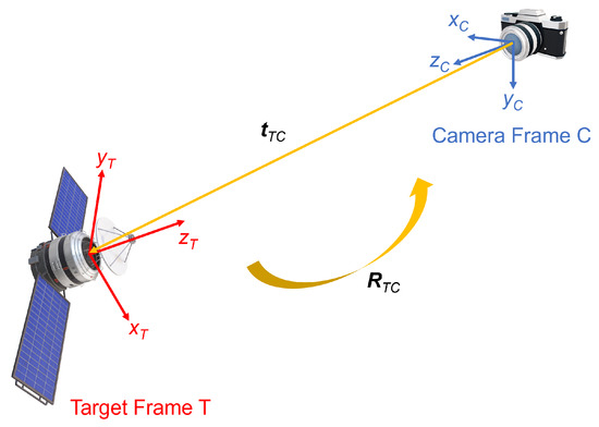
Figure 1.
Definitions of the target reference frame (T), camera reference frame (C), relative position (), and relative attitude ().
Figure 2 illustrates the overall pipeline of our method for known non-cooperative space target pose estimation via monocular images. We use a top-down method for landmark regression. Specifically, to solve the issues of scale variations, the bounding box of a space target is first detected in an input image, and then a sub-image is cropped from the image based on the box followed by a resize operation to a fixed size. The resized sub-image is then used to regress the locations of landmarks of the space target. Therefore, the 2D bounding boxes of space targets need to be detected first. To this end, we employ an off-the-shelf object detection network (e.g., R-CNN series [24,27,28,29,30,31,32], YOLO series [19,20,33,34,35,36], FCOS [37], RepPoints [38], and DETR series [39,40,41]) to detect space targets in an input image. Next, we propose a space target landmark regression network to predict the landmarks of a space target in the resized sub-image. Based on the 3D model of the known space target, we build 2D-3D correspondences between the 2D pixel coordinates in the input image and 3D space coordinates in the 3D model for landmarks of the space target. Given the putative 2D-3D correspondences, we use a PnP solver in [12] within the RANdom SAmple Consensus (RANSAC) [42] framework to recover the pose of the space target.
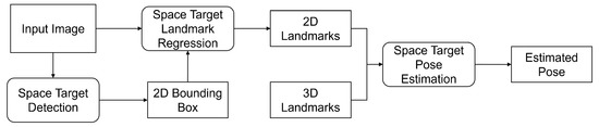
Figure 2.
The overall pipeline of monocular vision-based known non-cooperative space target pose estimation.
In this pipeline, the accuracy of landmark regression significantly affects the performance of pose estimation. However, current 2D heatmap representation is redundant for the sparse landmarks. In this article, we present a 1D landmark representation for landmark regression, which performs well on low-resolution images and requires no post-refinement steps.
3.1. 1D Landmark Representation
As shown in Figure 3, the representation of a landmark contains two independent fixed-length 1D vectors, which represent the horizontal and vertical pixel coordinates of the landmark separately. The generation process of 1D landmark representation will be described in detail in this section.
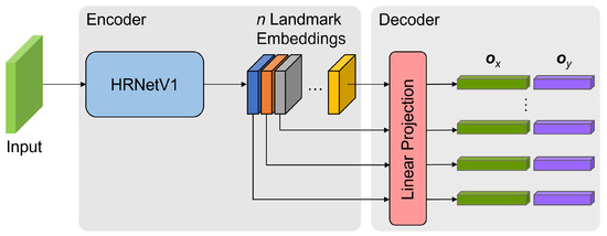
Figure 3.
The overall structure of the proposed space target landmark regression network.
The input image has a size of , where H and W are the height and width, respectively. The ground-truth 2D coordinate of the k-th landmark is denoted as , where is the horizontal coordinate subjected to , and is the vertical coordinate subjected to . To improve the accuracy of location description, we introduce an expansion factor , to adjust the scale of the landmark coordinate. Thus, the ground-truth 2D coordinate of the k-th landmark is transformed into a new 2D coordinate:
where is the round function, and is an integer subjected to . The proposed expansion factor can improve the localization accuracy to the level of sub-pixel. Then, the 1D landmark representation of the k-th landmark is defined as follows:
where , , and is the indicator function. Both and are 1D vectors. Such binary representation only encodes the 2D coordinate of a landmark while ignoring the adjacent point around the landmark. To describe the spatial relationships around landmarks, we introduce the Gaussian kernel to encode the 2D coordinates of landmarks and their surrounding points. For the k-th landmark, the Gaussian kernel-based 1D landmark representation is defined as follows:
where is the standard deviation.
In addition, the process of computing the 2D pixel coordinate of a landmark from 1D landmark representation is described as follows. Assuming the landmark regression network produces two 1D vectors and for a landmark, the final predicted 2D coordinate , of the landmark is computed by:
where denotes the i-th element of the , and denotes the j-th element of the .
3.2. Space Target Landmark Regression Network
We propose a top-down method to detect the landmarks of a space target in an input image. The input to the network is a fixed-size sub-image cropped from the input image using the detected bounding box. To enable the network to output 1D landmark representations, the network is designed to generate an embedding for each pre-defined landmark, and then use linear layers to project it into two 1D vectors with fixed lengths. As illustrated in Figure 3, we propose an encoder-decoder structured network to regress the locations of landmarks, where the encoder extracts landmark embeddings from the input, and the decoder predicts a 1D landmark representation for each landmark. The main modules of the proposed space target landmark regression network will be described in detail.
Encoder. To obtain high-quality landmark embeddings with rich spatial information, we use the HRNetV1 as described in [25,43] to extract embeddings for landmarks. Given n pre-defined landmarks, the output of HRNetV1 is a tensor of n embeddings corresponding one-to-one with landmarks only from the highest-resolution stream of the HRNetV1.
Decoder. The decoder comprises two shared linear projection layers that transform each embedding into a 1D landmark representation. Specifically, the embedding of a landmark is flattened and then fed into two shared fully-connected layers respectively to generate two independent 1D vectors and , with the lengths of and , respectively.
Loss function. Because the 1D landmark representation is similar to the one-hot code, the proposed space target landmark regression network could be considered to perform a kind of classification task. Therefore, we use the cross-entropy loss function to train the proposed network and adopt the label smoothing strategy to help train the network. The equation of the cross-entropy loss function is as follows.
where p is the input tensor with the size of , t is the target tensor with the size of , C is the number of classes, N is the batch size, and is the weight that is a 1D tensor of size C assigning weight to each of the classes. In addition, when using the Gaussian kernel-based 1D landmark representation in the proposed space target landmark regression network, we exploit the Kullback–Leibler divergence as the loss function for network training. The equation of the Kullback–Leibler divergence loss function is as follows.
where p is the input tensor and t is the target tensor, they have the same shape.
4. Material
We briefly introduce the dataset and evaluation metrics used in the experiment in this article.
4.1. Dataset
The Spacecraft PosE Estimation Dataset (SPEED) [13] is the first publicly available dataset for space target pose estimation, mostly consisting of high-resolution synthetic grayscale images of the Tango satellite, as shown in Figure 4. There are 12,000 training images with ground truth pose labels and 2998 test images without ground truth labels. The ground truth pose label consists of a unit quaternion and a translation vector, describing the relative orientation and position of the Tango satellite with respect to the camera frame.
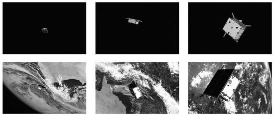
Figure 4.
Sample images from the SPEED.
Since SPEED does not provide the ground truth pose labels for test images, we cannot conduct an in-depth analysis over them except for acquiring the total pose error score provided by the online server. Therefore, we conduct extensive experiments on the training images, where half of them have no background while the other half contain earth backgrounds. Notably, the size and orientation of the satellite, background, and illumination vary significantly in these images. For instance, the number of pixels of the satellite varies between 1 k and 500 k, as shown in Figure 5.
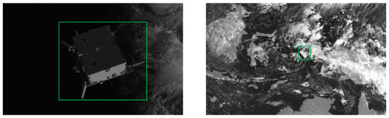
Figure 5.
Large variation of the space target size in the SPEED dataset.
The intrinsic parameters of the camera used in SPEED are the horizontal focal length of 0.0176 m, the vertical focal length of 0.0176 m, the horizontal pixel pitch of m/pixel, the vertical pixel pitch of m/pixel, the image width of 1920 pixel, and the image height of 1200 pixel.
4.2. Evaluation Metrics
We introduce the evaluation metrics for space target landmark regression and pose estimation.
4.2.1. Space Target Landmark Regression Metrics
To evaluate the performance of space target landmark regression, predictions are considered to be true or false positives by measuring distances between predicted and ground truth landmarks. Therefore, the Object Keypoint Similarity (OKS) [44] is calculated as following:
where is the Euclidean distance between the i-th landmark’s predicted and corresponding ground truth coordinates, is a constant, is the visibility flag, and s is the scale defined as the square root of the 2D bounding box area of the space target. For each landmark, this yields a similarity that ranges between 0 and 1. By setting a threshold for OKS, we can distinguish whether a prediction is a true positive or a false positive. Specifically, for each prediction, if the value of OKS is greater than the threshold, it is considered as a true positive, and vice versa. Then, we can compute precision as following:
In addition, there may be ground truth landmarks with no matching predictions, so they are called false negatives. Thus, we also need to compute recall as following:
Then, the precision-recall curve is calculated to compute the average precision value, as described in [45].
The Average Precision (AP) [45] is used as the space target landmark regression metric. For better measuring the performances of methods, it is averaged over multiple OKS values [44]. Specifically, is computed at 10 OKS thresholds from 0.50 to 0.95 with a step size of 0.05, is computed at a single OKS threshold of 0.50, and is computed at a single OKS threshold of 0.75.
4.2.2. Space Target Pose Estimation Metrics
To evaluate the estimated pose of each space target, a rotation error , a translation error , and a pose error , are calculated.
The rotation error , is calculated as the angular distance between the estimated and ground-truth rotation quaternions and , of a space target with respect to the camera. The rotation error , is defined as
where denotes the inner product operation.
The translation error , is calculated as the 2-norm of the difference of the estimated and ground-truth translation vectors and , from the camera frame to the space target frame. The translation error , is defined as
The normalized translation error , is also defined as
which penalizes the translation error more heavily when the space target is closer to the camera.
The pose error for a single space target , is the sum of the rotation error , and the normalized translation error ,
Finally, the total error E is the average of the pose errors for all space targets,
where N is the number of space targets.
5. Experimental Results
In this section, we first give the details of the experiment, then we evaluate the performance of our method and compare it with several state-of-the-art methods.
5.1. Experiment Details
As a preliminary, since the 3D model of the Tango satellite is unavailable in SPEED, we first reconstruct the 3D landmarks of the Tango satellite via multi-view triangulation using a small set of manually selected training images with pose labels. Moreover, to obtain ground-truth 2D bounding boxes and landmarks, we first project the reconstructed 3D landmarks of the Tango satellite into the image to obtain the 2D landmark labels and then extract the closest bounding box of the reprojected points as the label for 2D object detection. Finally, we briefly introduce the implementation details of the experiment.
5.1.1. 3D Landmark Reconstruction
For Tango satellite, we select its 8 corners and the tips of its 3 antennas as landmarks. To reconstruct the 3D coordinates of the 11 landmarks using multi-view triangulation, we manually annotate 2D points corresponding to each landmark over a small set of hand-picked close-up training images in which the space target is well-illuminated and has various poses. Assuming is the 2D coordinate vector of the i-th landmark in the j-th image, the following optimization problem is solved to obtain the 3D coordinate vector of the i-th landmark , in the space target frame,
where, for i-th landmark, the sum of the reprojection error is minimized over a set of images where the i-th landmark is visible. In Equation (19), is a scale factor denoting the depth of the i-th landmark in the j-th image, is a known camera intrinsic matrix, and is a ground truth camera pose of the j-th image. The optimization variable in Equation (19) is the 3D coordinate vector . The routine of the triangulateMultiview function in MATLAB is used to solve this optimization problem. Figure 6 visualizes the 11 selected 3D landmarks and the reconstructed wireframe model of the Tango satellite.
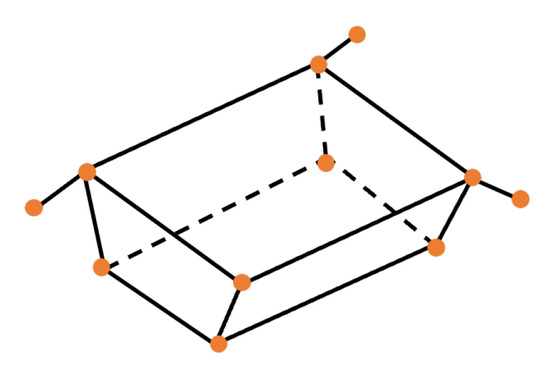
Figure 6.
The reconstructed 3D wireframe model with 11 landmarks.
5.1.2. 2D Landmark and Bounding Box Label
To obtain ground-truth landmarks of the Tango satellite in the image, we reproject the aforementioned set of reconstructed 3D landmarks to the image plane using the ground-truth camera pose. Since the convex hull of such reprojected 2D landmarks almost covers the whole target in any image, we slightly relax the horizontal rectangle which encloses all 2D landmarks, and take it as the ground-truth bounding box of the Tango satellite. Figure 7 shows several examples of obtained 2D landmark and bounding box labels.
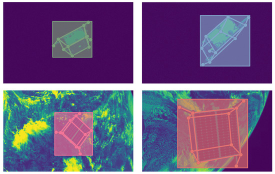
Figure 7.
Examples of 2D landmark and bounding box labels.
5.1.3. Implementation Details
We conduct experiments using 6-fold cross-validation over the training images of the SPEED dataset. Specifically, we split the 12,000 training images into 6 groups, and then for each group, we test a space target landmark regression network trained with the remaining 5 groups. In addition, we use the off-the-shelf object detection network Sparse R-CNN [32] to detect 2D bounding boxes. The neural network architecture is implemented with PyTorch 1.11.0 and CUDA 11.3 and runs on an Intel Core i9-10900X CPU @ 3.70 GHz with an NVIDIA Geforce RTX 3090. The pose estimation algorithm is implemented with MATLAB.
Data augmentation. To increase the diversity of training samples and alleviate the accuracy error of the detected 2D bounding boxes, we introduce a bounding box augmentation strategy which random shifts bounding box centers slightly while the targets are still within bounding boxes. What is more, we also use data augmentation strategies such as random rotation () and random scaling () for training images. We do not apply a random flipping strategy to the training images because it might generate unrealistic geometric relationships between 2D landmarks, which may result in performance degradation of networks.
Training setting. We use the Adam optimizer [46] for network training. The base learning rate is set to , and is dropped to and at the 16th and 22nd epochs, respectively. The total training process is terminated within 24 epochs. The batch contains 8 randomly sampled samples per iteration. The HRNetV1 backbone in the proposed space target landmark regression network is initialized with a pre-trained model HRNetV1-W32 [43] which is pretrained with the COCO dataset [44].
5.2. Results of Space Target Landmark Regression
As shown in Table 1, we evaluate the performance of our proposed space target landmark regression network in terms of the , , and metrics. In this experiment, we set up the expansion factor as 2 and the standard deviation of the Gaussian kernel , as 2. For each fold, we test the performances of the proposed space target landmark regression network using 1D landmark representations with or without Gaussian kernel at four input resolutions including , , , and . The AP is improved as the input resolution increases, no matter whether the Gaussian kernel is used in the 1D landmark representation. When the Gaussian kernel is introduced into the 1D landmark representation, the AP is commonly superior to the one without the Gaussian kernel at any input resolution. It empirically demonstrates that spatial relationships play an important role in describing the coordinates of landmarks and improve the performances of landmark regression networks. Figure 8 shows qualitative results where the orange points are the landmarks predicted by the proposed landmark regression network using Gaussian kernel-based 1D landmark representations at the input resolution of .

Table 1.
Quantitative results of space target landmark regression and pose estimation using the proposed 1D landmark representation.
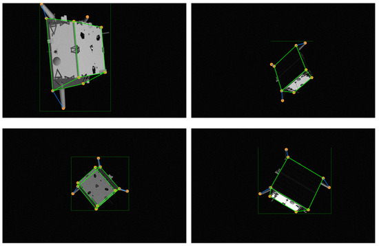
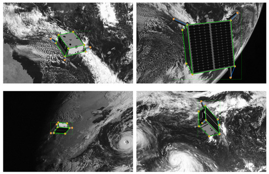
Figure 8.
Qualitative results for the proposed space target landmark regression network using Gaussian kernel-based 1D landmark representations at the input resolution of .
5.3. Results of Space Target Pose Estimation
As shown in Table 1, we evaluate the performance of space target pose estimation that uses 2D landmarks predicted by our proposed space target landmark regression network. The evaluation metrics for space target pose estimation are composed as follows. is the average of the rotation errors for all space targets. is the average of the normalized translation errors for all space targets. E is the total error which is the sum of and . For each fold, all kinds of errors decrease as the input resolution increases. What is more, estimating spatial target pose using predicted landmarks described by the Gaussian kernel-based 1D landmark representation generally leads to a performance boost. Figure 9 shows qualitative results of space target pose estimation using predicted landmarks based on the Gaussian kernel-based 1D landmark representation under the input resolution condition of . The satellite body frame’s correspondence between colors and directions is red—x, green—y, and blue—z.
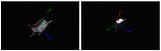
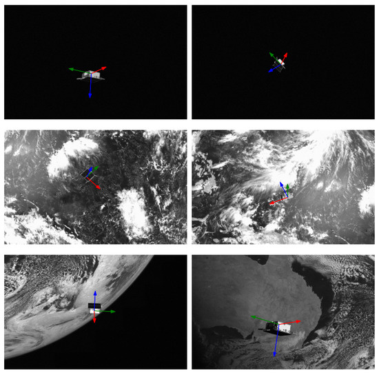
Figure 9.
Qualitative results for space target pose estimation using 2D landmarks predicted by the proposed space target landmark regression network using Gaussian kernel-based 1D landmark representations at the input resolution of .
5.4. Comparisons with State-of-the-Art Methods
We compare our method with the state-of-the-art methods in space target landmark regression and pose estimation. To compare with them, we re-implement the same pipeline as [7,8], both of which estimate the poses of space targets by regressing the pre-defined landmarks of space targets in images.
5.4.1. Performance of Space Target Landmark Regression
To evaluate the performance of space target landmark regression, we compare our method with [7,8] in terms of the , , and metrics. In [7], the coordinates of landmarks are directly regressed by the network using Darknet53 [20] as the backbone. In [8], HRNetV1-W32 [43] is used to produce heatmaps for landmarks, and then the coordinates of landmarks are calculated by post-processing on these heatmaps. It should be pointed out that we use pre-trained models which are pretrained on the COCO dataset [44] to initialize the weights of Darknet53 and HRNetV1-W32 during training re-implemented networks. In our proposed method, both the expansion factor and standard deviation of the Gaussian kernel are defined as 2. Table 2 presents the comparison between our method and the state-of-the-art methods, in which each of the values of a metric is the average over the values for the metric from all over the folds. As shown in Table 2, our methods outperform the direct regression method [7] at any input size condition. Our methods achieve the same level of AP as the heatmap regression method [8] for the input sizes of and , respectively. When the input size decreases to and , our method without Gaussian kernel gets 89.9 and 70.3 AP, respectively, which have 6.8 and 33.5 improvements compared to the heatmap regression method [8], while the one with Gaussian kernel gets 91.0 and 74.0 AP, respectively, which achieve 7.9 and 37.2 improvements in contrast to the heatmap regression method [8]. Meanwhile, our methods have similar model sizes and GFLOPs to the heatmap regression method [8].
Table 2.
Comparison with the state-of-the-art methods in terms of the evaluation metrics for space target landmark regression.
Figure 10 illustrates that our methods consistently provide significant gains for the performance of space target landmark regression, especially in low-resolution input conditions. Whereas, both the direct regression method [7] and the heatmap regression method [8] suffer from drastic performance drop as the input size degrades.
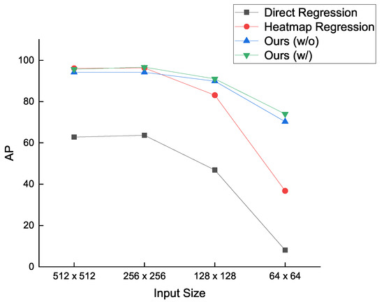
Figure 10.
Comparison between our methods and the state-of-the-art methods in terms of the AP metric at all input size conditions.
5.4.2. Performance of Space Target Pose Estimation
To evaluate the performance of space target pose estimation that uses predicted 2D landmarks to recover the pose of a space target, we compare our method with [7,8] in terms of , , and E metrics. Furthermore, in order to investigate the impact of 2D landmarks predicted by various methods on space target pose estimation, we universally use the RANSAC-based PnP solver [12] instead of the improved PnP algorithm as described in [8] to compute space target poses. Table 3 presents the comparison between our method and the state-of-the-art methods, where the values of each metric are all the averages of the values of the metric from all folds. As shown in Table 3, our methods achieve smaller pose error than the direct regression method [7] and the heatmap regression method [8] under any input size condition. Compared with the heatmap regression method [8], our methods without and with Gaussian kernel get little gains for the input size of while attaining increasing gains as the input size decreases. Especially, at the input size of , the total errors of our methods without and with Gaussian kernel are lower by 0.1571 and 0.1657, respectively.
Table 3.
Comparison with the state-of-the-art methods for space target pose estimation.
Figure 11 illustrates that our proposed methods maintain a low error level of space target pose estimation for any input size. However, the total errors of the direct regression method [7] and the heatmap regression method [8] increase sharply when the input size decreases. In particular, the total error of the direct regression method [7] is the largest among all methods at any input size.
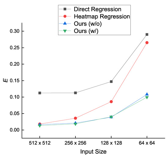
Figure 11.
Comparison between our methods and the state-of-the-art methods in terms of the E metric at all input size conditions.
6. Discussion
We give a discussion on the property of 1D landmark representation compared to the 2D heatmap representation. The discussion is conducted from the perspectives of complexity and quantization error. In addition, we conduct an analysis on the expansion factor .
6.1. Representation Complexity
Given an input image with the resolution of , heatmap regression methods aim to generate a 2D heatmap with the resolution of , where is the downsampling factor. Since is a constant, the spatial complexity of the heatmap representation is . Whereas, our method aims to yield two 1D vectors with the length of and respectively, where is the expansion factor. Considering is a constant, the spatial complexity of the proposed 1D landmark representation is . Therefore, we can find that the 1D landmark representation is more efficient than the heatmap representation. Particularly, it enables some methods to remove extra independent upsampling operations (e.g., deconvolution [11]) used to obtain high-resolution landmark embeddings directly so that the computational costs of networks can be reduced.
6.2. Quantization Error
Given an input image with the resolution of and the ground-truth 2D coordinate of a landmark , we take the horizontal coordinate x, as an example to analyze the quantization errors of 1D landmark representation and 2D heatmap representation, respectively.
For 1D landmark representation, x can be rewritten as:
where is the expansion factor subjected to , , , and . The ground-truth x is then rescaled by into a new one:
The quantization error of 1D landmark representation , is calculated as:
Therefore, the quantization error of 1D landmark representation , satisfies .
For heatmap representation, x can be rewritten as:
where is the downsampling factor subjected to , , . Due to that the heatmap resolution is usually downsampled from the original input image resolution, the ground-truth x is transformed as:
The quantization error of heatmap representation , is calculated as:
Therefore, the quantization error of heatmap representation , satisfies .
This reduces the quantization error from the level of to the level of . In order to alleviate the quantization error of heatmap representation, extra time-consuming refinements are always employed. In contrast, 1D landmark representation does not require extra coordinate post-processing and reduce the quantization error, which promote the improvement of space target landmark regression.
6.3. Analysis on Expansion Factor
The expansion factor, , is the only hyperparameter in the 1D landmark representation, which controls the sub-pixel accuracy level of the landmark location. Specifically, the larger is, the lower the quantization error of 1D landmark representation is. Nevertheless, the increase in the expansion factor brings more computational burden to network training. Therefore, there is a trade-off between the quantization error and the network performance. We test in the 1D landmark representation without Gaussian kernel based on the proposed space target landmark regression network at various input resolutions. As shown in Figure 12, the performance of the proposed network tends to decrease as increases. For the input sizes of and , the best choice to is 1 so that the proposed network achieves the AP of 72.4 and 90.5, respectively. For the input sizes of and , the value of affects the network performance indistinctively. Specifically, the proposed network achieves the best AP of 94.4 and 94.6 when is set up as 1.
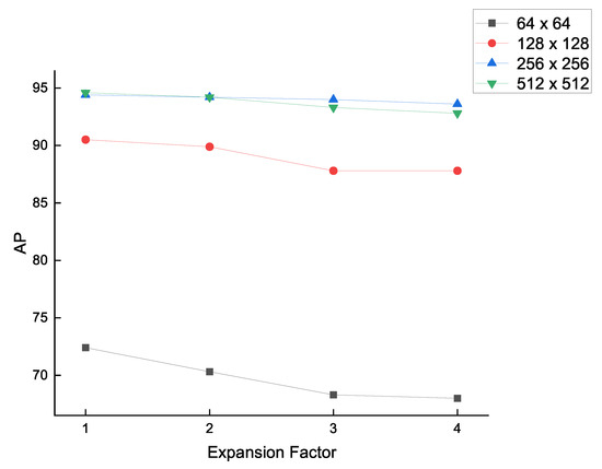
Figure 12.
Analysis of the value of expansion factor , under various input resolution conditions.
7. Conclusions
In this article, we study the task of the space target pose estimation from monocular images and propose a novel approach. Based on the 2D-3D correspondences-based pose estimation pipeline, we present a 1D landmark representation to describe the 2D coordinates of pre-defined landmarks in images, to deal with several drawbacks of the 2D heatmap representation that dominates the landmark regression task. Next, we propose a space target landmark regression network to predict the horizontal and vertical coordinates of landmarks respectively using 1D landmark representations. Experimental results on the SPEED dataset show that our method achieves superior performance to the existing state-of-the-art methods in space target landmark regression and pose estimation, especially when the input images are low in resolution. In the space target landmark regression task, our method using the 1D landmark representation without Gaussian kernel achieves 70.3, 89.9, 94.2, and 94.2 AP respectively at the input sizes of , , , and , while using the Gaussian kernel-based 1D landmark representation, our method achieves 74.0, 91.0, 96.7, and 95.7 AP respectively. In the space target pose estimation task, the total errors of our method using the 1D landmark representation without Gaussian kernel are 0.1082, 0.0390, 0.0209, and 0.0163 respectively at the input sizes of , , , and , while using the Gaussian kernel-based 1D landmark representation, the total errors of our method are 0.0996, 0.0401, 0.0186, and 0.0135 respectively. Furthermore, we discuss the property of the proposed 1D landmark representation, which has less computational complexity and quantization error than the 2D heatmap. We also analyze the settings of the value of expansion factor at various input resolutions. In particular, for the input sizes of and , the best choice for the value of the expansion factor is 1, while for the input sizes of and , the value of the expansion factor affects the network performance indistinctively. In the future, we would like to adopt more geometric information such as the edges, parts, and structures of space targets to our method and extend our approach to other targets, such as aircraft and vehicles.
Author Contributions
Conceptualization, S.L. and G.W.; methodology, S.L.; software, S.L.; validation, S.L., X.Z., Z.C. and G.W.; formal analysis, S.L.; investigation, S.L.; resources, S.L.; data curation, S.L.; writing—original draft preparation, S.L.; writing—review and editing, X.Z. and Z.C.; visualization, S.L.; supervision, G.W.; project administration, G.W.; funding acquisition, G.W. All authors have read and agreed to the published version of the manuscript.
Funding
This research was funded by the National Natural Science Foundation of China (No. 62106283) and the Natural Science Foundation of Shaanxi Province (No. 2021JM-226).
Data Availability Statement
The SPEED dataset is available at https://kelvins.esa.int/satellite-pose-estimation-challenge/ (accessed on 12 July 2022).
Acknowledgments
We thank the Advanced Concepts Team (ACT) of the European Space Agency and the Space Rendezvous Laboratory (SLAB) of Stanford University for providing the Spacecraft PosE Estimation Dataset (SPEED) online.
Conflicts of Interest
The authors declare no conflict of interest.
References
- Chen, L.; Li, S.; Bai, Q.; Yang, J.; Jiang, S.; Miao, Y. Review of Image Classification Algorithms Based on Convolutional Neural Networks. Remote Sens. 2021, 13, 4712. [Google Scholar] [CrossRef]
- Zaidi, S.S.A.; Ansari, M.S.; Aslam, A.; Kanwal, N.; Asghar, M.N.; Lee, B. A survey of modern deep learning based object detection models. Digit. Signal Process. 2022, 126, 103514. [Google Scholar] [CrossRef]
- Mo, Y.; Wu, Y.; Yang, X.; Liu, F.; Liao, Y. Review the state-of-the-art technologies of semantic segmentation based on deep learning. Neurocomputing 2022, 493, 626–646. [Google Scholar] [CrossRef]
- Sharma, S.; Beierle, C.; D’Amico, S. Pose estimation for non-cooperative spacecraft rendezvous using convolutional neural networks. In Proceedings of the 2018 IEEE Aerospace Conference, Big Sky, MT, USA, 3–10 March 2018; pp. 1–12. [Google Scholar]
- Proença, P.F.; Gao, Y. Deep Learning for Spacecraft Pose Estimation from Photorealistic Rendering. In Proceedings of the 2020 IEEE International Conference on Robotics and Automation (ICRA 2020), Paris, France, 31 May–31 August 2020; pp. 6007–6013. [Google Scholar]
- Sharma, S.; D’Amico, S. Neural Network-Based Pose Estimation for Noncooperative Spacecraft Rendezvous. IEEE Trans. Aerosp. Electron. Syst. 2020, 56, 4638–4658. [Google Scholar] [CrossRef]
- Park, T.H.; Sharma, S.; D’Amico, S. Towards Robust Learning-Based Pose Estimation of Noncooperative Spacecraft. arXiv 2019, arXiv:1909.00392. [Google Scholar]
- Chen, B.; Cao, J.; Bustos, Á.P.; Chin, T. Satellite Pose Estimation with Deep Landmark Regression and Nonlinear Pose Refinement. In Proceedings of the 2019 IEEE/CVF International Conference on Computer Vision Workshops (ICCV Workshops 2019), Seoul, Korea, 27–28 October 2019; pp. 2816–2824. [Google Scholar]
- Xu, J.; Song, B.; Yang, X.; Nan, X. An Improved Deep Keypoint Detection Network for Space Targets Pose Estimation. Remote Sens. 2020, 12, 3857. [Google Scholar] [CrossRef]
- Hu, Y.; Speierer, S.; Jakob, W.; Fua, P.; Salzmann, M. Wide-Depth-Range 6D Object Pose Estimation in Space. In Proceedings of the IEEE Conference on Computer Vision and Pattern Recognition (CVPR 2021), Virtual, 19–25 June 2021; pp. 15870–15879. [Google Scholar]
- Noh, H.; Hong, S.; Han, B. Learning Deconvolution Network for Semantic Segmentation. In Proceedings of the 2015 IEEE International Conference on Computer Vision (ICCV 2015), Santiago, Chile, 7–13 December 2015; pp. 1520–1528. [Google Scholar]
- Gao, X.; Hou, X.; Tang, J.; Cheng, H. Complete Solution Classification for the Perspective-Three-Point Problem. IEEE Trans. Pattern Anal. Mach. Intell. 2003, 25, 930–943. [Google Scholar] [CrossRef]
- Kisantal, M.; Sharma, S.; Park, T.H.; Izzo, D.; Märtens, M.; D’Amico, S. Satellite Pose Estimation Challenge: Dataset, Competition Design, and Results. IEEE Trans. Aerosp. Electron. Syst. 2020, 56, 4083–4098. [Google Scholar] [CrossRef]
- Krizhevsky, A.; Sutskever, I.; Hinton, G.E. ImageNet Classification with Deep Convolutional Neural Networks. In Proceedings of the 26th Annual Conference on Neural Information Processing Systems, Lake Tahoe, NV, USA, 3–6 December 2012; pp. 1106–1114. [Google Scholar]
- He, K.; Zhang, X.; Ren, S.; Sun, J. Deep Residual Learning for Image Recognition. In Proceedings of the 2016 IEEE Conference on Computer Vision and Pattern Recognition (CVPR 2016), Las Vegas, NV, USA, 27–30 June 2016; pp. 770–778. [Google Scholar]
- Li, S.; Xu, C. A Stable Direct Solution of Perspective-Three-Point Problem. Int. J. Pattern Recognit. Artif. Intell. 2011, 25, 627–642. [Google Scholar] [CrossRef]
- Li, S.; Xu, C.; Xie, M. A Robust O(n) Solution to the Perspective-n-Point Problem. IEEE Trans. Pattern Anal. Mach. Intell. 2012, 34, 1444–1450. [Google Scholar] [CrossRef] [PubMed]
- Lepetit, V.; Moreno-Noguer, F.; Fua, P. EPnP: An Accurate O(n) Solution to the PnP Problem. Int. J. Comput. Vis. 2009, 81, 155–166. [Google Scholar] [CrossRef]
- Redmon, J.; Farhadi, A. YOLO9000: Better, Faster, Stronger. In Proceedings of the 2017 IEEE Conference on Computer Vision and Pattern Recognition (CVPR 2017), Honolulu, HI, USA, 21–26 July 2017; pp. 6517–6525. [Google Scholar]
- Redmon, J.; Farhadi, A. YOLOv3: An Incremental Improvement. arXiv 2018, arXiv:1804.02767. [Google Scholar]
- Howard, A.G.; Zhu, M.; Chen, B.; Kalenichenko, D.; Wang, W.; Weyand, T.; Andreetto, M.; Adam, H. MobileNets: Efficient Convolutional Neural Networks for Mobile Vision Applications. arXiv 2017, arXiv:1704.04861. [Google Scholar]
- Sandler, M.; Howard, A.G.; Zhu, M.; Zhmoginov, A.; Chen, L. MobileNetV2: Inverted Residuals and Linear Bottlenecks. In Proceedings of the 2018 IEEE Conference on Computer Vision and Pattern Recognition (CVPR 2018), Salt Lake City, UT, USA, 18–22 June 2018; pp. 4510–4520. [Google Scholar]
- Lin, T.; Dollár, P.; Girshick, R.B.; He, K.; Hariharan, B.; Belongie, S.J. Feature Pyramid Networks for Object Detection. In Proceedings of the 2017 IEEE Conference on Computer Vision and Pattern Recognition (CVPR 2017), Honolulu, HI, USA, 21–26 July 2017; pp. 936–944. [Google Scholar]
- Ren, S.; He, K.; Girshick, R.B.; Sun, J. Faster R-CNN: Towards Real-Time Object Detection with Region Proposal Networks. IEEE Trans. Pattern Anal. Mach. Intell. 2017, 39, 1137–1149. [Google Scholar] [CrossRef] [PubMed]
- Sun, K.; Xiao, B.; Liu, D.; Wang, J. Deep High-Resolution Representation Learning for Human Pose Estimation. In Proceedings of the IEEE Conference on Computer Vision and Pattern Recognition (CVPR 2019), Long Beach, CA, USA, 16–20 June 2019; pp. 5693–5703. [Google Scholar]
- Wang, Z.; Zhang, Z.; Sun, X.; Li, Z.; Yu, Q. Revisiting Monocular Satellite Pose Estimation with Transformer. IEEE Trans. Aerosp. Electron. Syst. 2022. [Google Scholar] [CrossRef]
- He, K.; Gkioxari, G.; Dollár, P.; Girshick, R.B. Mask R-CNN. In Proceedings of the IEEE International Conference on Computer Vision (ICCV 2017), Venice, Italy, 22–29 October 2017; pp. 2980–2988. [Google Scholar]
- Cai, Z.; Vasconcelos, N. Cascade R-CNN: Delving Into High Quality Object Detection. In Proceedings of the 2018 IEEE Conference on Computer Vision and Pattern Recognition (CVPR 2018), Salt Lake City, UT, USA, 18–22 June 2018; pp. 6154–6162. [Google Scholar]
- Pang, J.; Chen, K.; Shi, J.; Feng, H.; Ouyang, W.; Lin, D. Libra R-CNN: Towards Balanced Learning for Object Detection. In Proceedings of the IEEE Conference on Computer Vision and Pattern Recognition (CVPR 2019), Long Beach, CA, USA, 16–20 June 2019; pp. 821–830. [Google Scholar]
- Wu, Y.; Chen, Y.; Yuan, L.; Liu, Z.; Wang, L.; Li, H.; Fu, Y. Rethinking Classification and Localization for Object Detection. In Proceedings of the 2020 IEEE/CVF Conference on Computer Vision and Pattern Recognition (CVPR 2020), Seattle, WA, USA, 13–19 June 2020; pp. 10183–10192. [Google Scholar]
- Zhang, H.; Chang, H.; Ma, B.; Wang, N.; Chen, X. Dynamic R-CNN: Towards High Quality Object Detection via Dynamic Training. In Proceedings of the Computer Vision—ECCV 2020—16th European Conference, Glasgow, UK, 23–28 August 2020; pp. 260–275. [Google Scholar]
- Sun, P.; Zhang, R.; Jiang, Y.; Kong, T.; Xu, C.; Zhan, W.; Tomizuka, M.; Li, L.; Yuan, Z.; Wang, C.; et al. Sparse R-CNN: End-to-End Object Detection With Learnable Proposals. In Proceedings of the IEEE Conference on Computer Vision and Pattern Recognition (CVPR 2021), Virtual, 19–25 June 2021; pp. 14454–14463. [Google Scholar]
- Redmon, J.; Divvala, S.K.; Girshick, R.B.; Farhadi, A. You Only Look Once: Unified, Real-Time Object Detection. In Proceedings of the 2016 IEEE Conference on Computer Vision and Pattern Recognition (CVPR 2016), Las Vegas, NV, USA, 27–30 June 2016; pp. 779–788. [Google Scholar]
- Bochkovskiy, A.; Wang, C.; Liao, H.M. YOLOv4: Optimal Speed and Accuracy of Object Detection. arXiv 2020, arXiv:2004.10934. [Google Scholar]
- Chen, Q.; Wang, Y.; Yang, T.; Zhang, X.; Cheng, J.; Sun, J. You Only Look One-Level Feature. In Proceedings of the IEEE Conference on Computer Vision and Pattern Recognition (CVPR 2021), Virtual, 19–25 June 2021; pp. 13039–13048. [Google Scholar]
- Ge, Z.; Liu, S.; Wang, F.; Li, Z.; Sun, J. YOLOX: Exceeding YOLO Series in 2021. arXiv 2021, arXiv:2107.08430. [Google Scholar]
- Tian, Z.; Shen, C.; Chen, H.; He, T. FCOS: Fully Convolutional One-Stage Object Detection. In Proceedings of the 2019 IEEE/CVF International Conference on Computer Vision (ICCV 2019), Seoul, Korea, 27 October–2 November 2019; pp. 9626–9635. [Google Scholar]
- Yang, Z.; Liu, S.; Hu, H.; Wang, L.; Lin, S. RepPoints: Point Set Representation for Object Detection. In Proceedings of the 2019 IEEE/CVF International Conference on Computer Vision (ICCV 2019), Seoul, Korea, 27 October–2 November 2019; pp. 9656–9665. [Google Scholar]
- Carion, N.; Massa, F.; Synnaeve, G.; Usunier, N.; Kirillov, A.; Zagoruyko, S. End-to-End Object Detection with Transformers. In Proceedings of the Computer Vision—ECCV 2020—16th European Conference, Glasgow, UK, 23–28 August 2020; pp. 213–229. [Google Scholar]
- Zhu, X.; Su, W.; Lu, L.; Li, B.; Wang, X.; Dai, J. Deformable DETR: Deformable Transformers for End-to-End Object Detection. In Proceedings of the 9th International Conference on Learning Representations (ICLR 2021), Virtual Event, 3–7 May 2021. [Google Scholar]
- Dai, X.; Chen, Y.; Yang, J.; Zhang, P.; Yuan, L.; Zhang, L. Dynamic DETR: End-to-End Object Detection with Dynamic Attention. In Proceedings of the 2021 IEEE/CVF International Conference on Computer Vision (ICCV 2021), Montreal, QC, Canada, 10–17 October 2021; pp. 2968–2977. [Google Scholar]
- Fischler, M.A.; Bolles, R.C. Random Sample Consensus: A Paradigm for Model Fitting with Applications to Image Analysis and Automated Cartography. Commun. ACM 1981, 24, 381–395. [Google Scholar] [CrossRef]
- Wang, J.; Sun, K.; Cheng, T.; Jiang, B.; Deng, C.; Zhao, Y.; Liu, D.; Mu, Y.; Tan, M.; Wang, X.; et al. Deep High-Resolution Representation Learning for Visual Recognition. IEEE Trans. Pattern Anal. Mach. Intell. 2021, 43, 3349–3364. [Google Scholar] [CrossRef] [PubMed]
- Lin, T.; Maire, M.; Belongie, S.J.; Hays, J.; Perona, P.; Ramanan, D.; Dollár, P.; Zitnick, C.L. Microsoft COCO: Common Objects in Context. In Proceedings of the Computer Vision—ECCV 2014—13th European Conference, Zurich, Switzerland, 6–12 September 2014; pp. 740–755. [Google Scholar]
- Everingham, M.; Eslami, S.M.A.; Gool, L.V.; Williams, C.K.I.; Winn, J.M.; Zisserman, A. The Pascal Visual Object Classes Challenge: A Retrospective. Int. J. Comput. Vis. 2015, 111, 98–136. [Google Scholar] [CrossRef]
- Kingma, D.P.; Ba, J. Adam: A Method for Stochastic Optimization. In Proceedings of the 3rd International Conference on Learning Representations (ICLR 2015), San Diego, CA, USA, 7–9 May 2015. [Google Scholar]
Publisher’s Note: MDPI stays neutral with regard to jurisdictional claims in published maps and institutional affiliations. |
© 2022 by the authors. Licensee MDPI, Basel, Switzerland. This article is an open access article distributed under the terms and conditions of the Creative Commons Attribution (CC BY) license (https://creativecommons.org/licenses/by/4.0/).