
Evaluating Satellite Soil Moisture Datasets for Drought Monitoring in Australia and the South-West Pacific

 ,
, _Sun.png)
Abstract
:
1. Introduction
2. Data and Methods
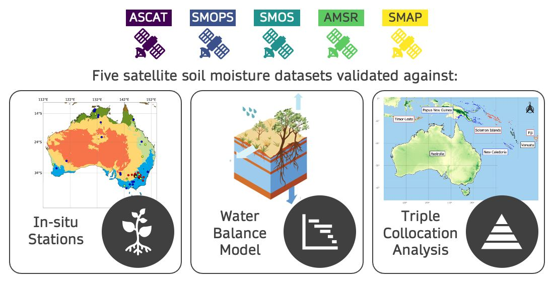
2.1. Satellite Datasets
2.1.1. ASCAT
2.1.2. SMOPS
2.1.3. SMOS
2.1.4. AMSR-2
2.1.5. SMAP
2.2. Validation Metrics
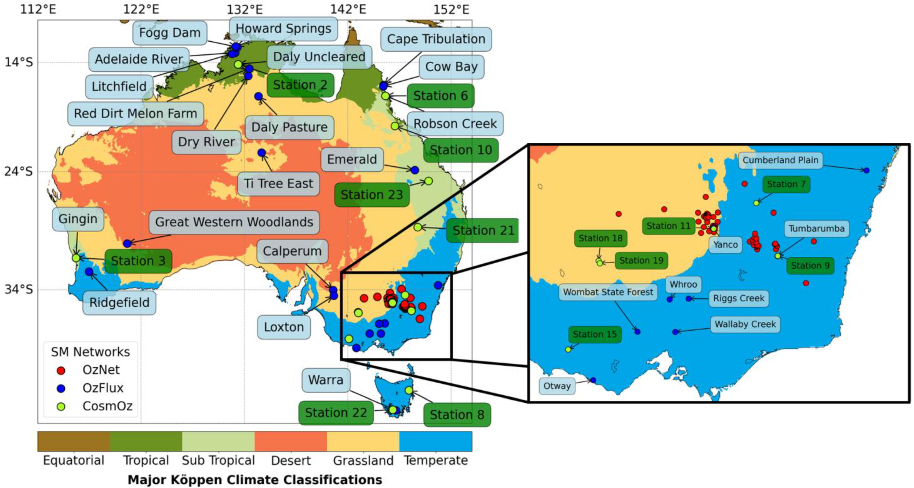
2.3. Point-Based Analysis Datasets
2.3.1. OzNet
2.3.2. CosmOz
2.3.3. OzFlux
2.4. Gridded Analysis—AWRA-L
2.5. Triple Collocation Analysis

2.5.1. GLDAS
2.5.2. ERA5-Land
2.6. Agrometeorological Drought Case Study
3. Results
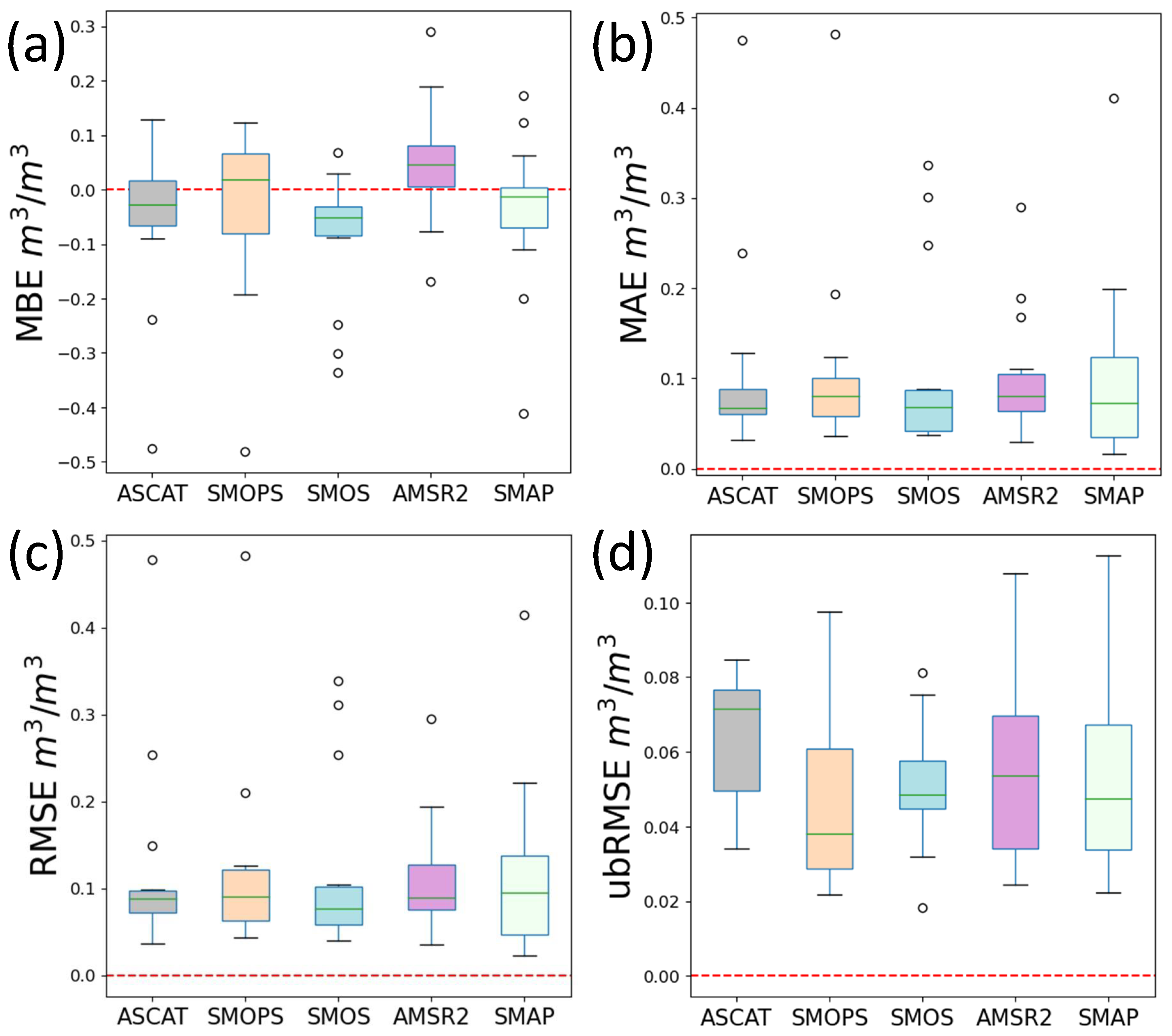
3.1. Point-Based Analysis
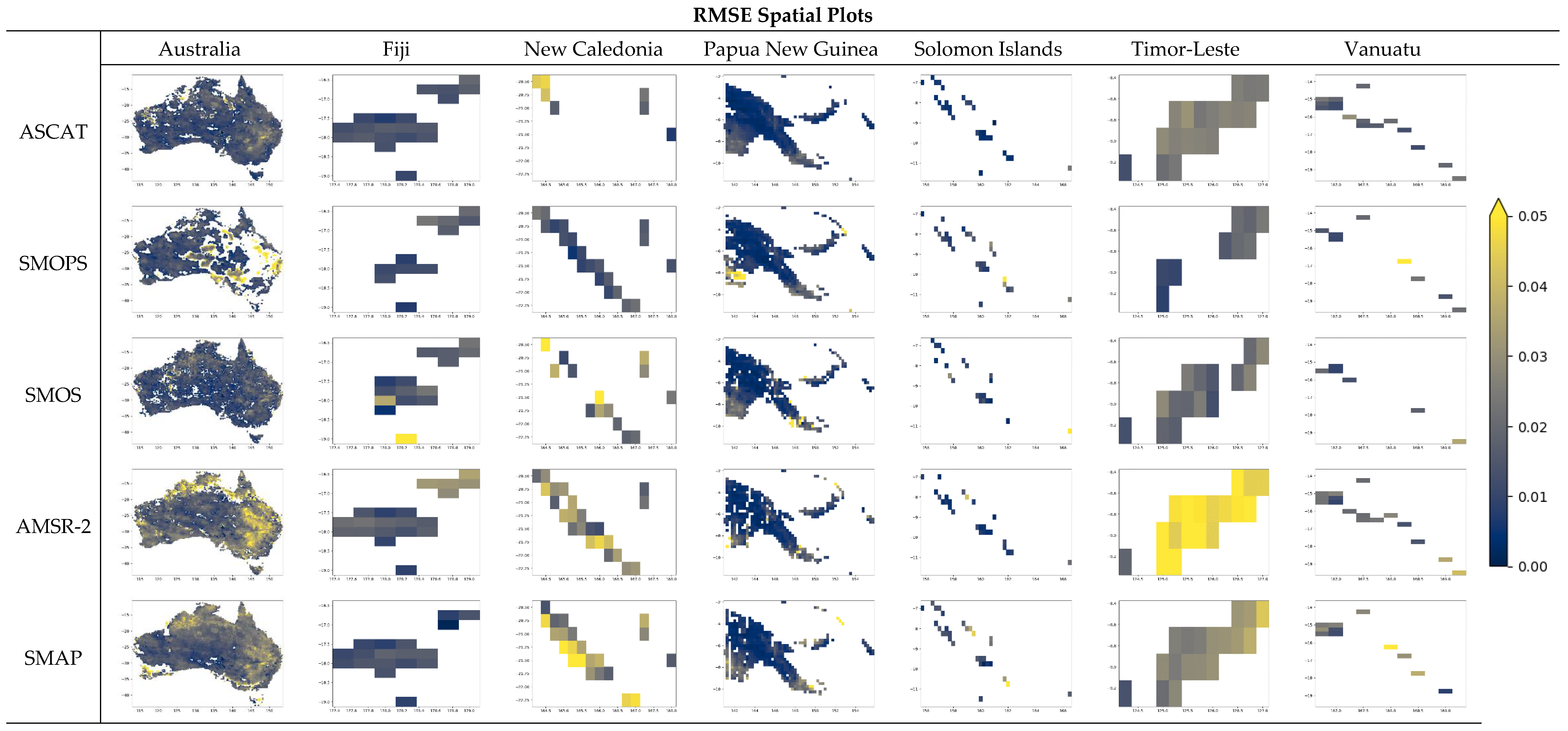
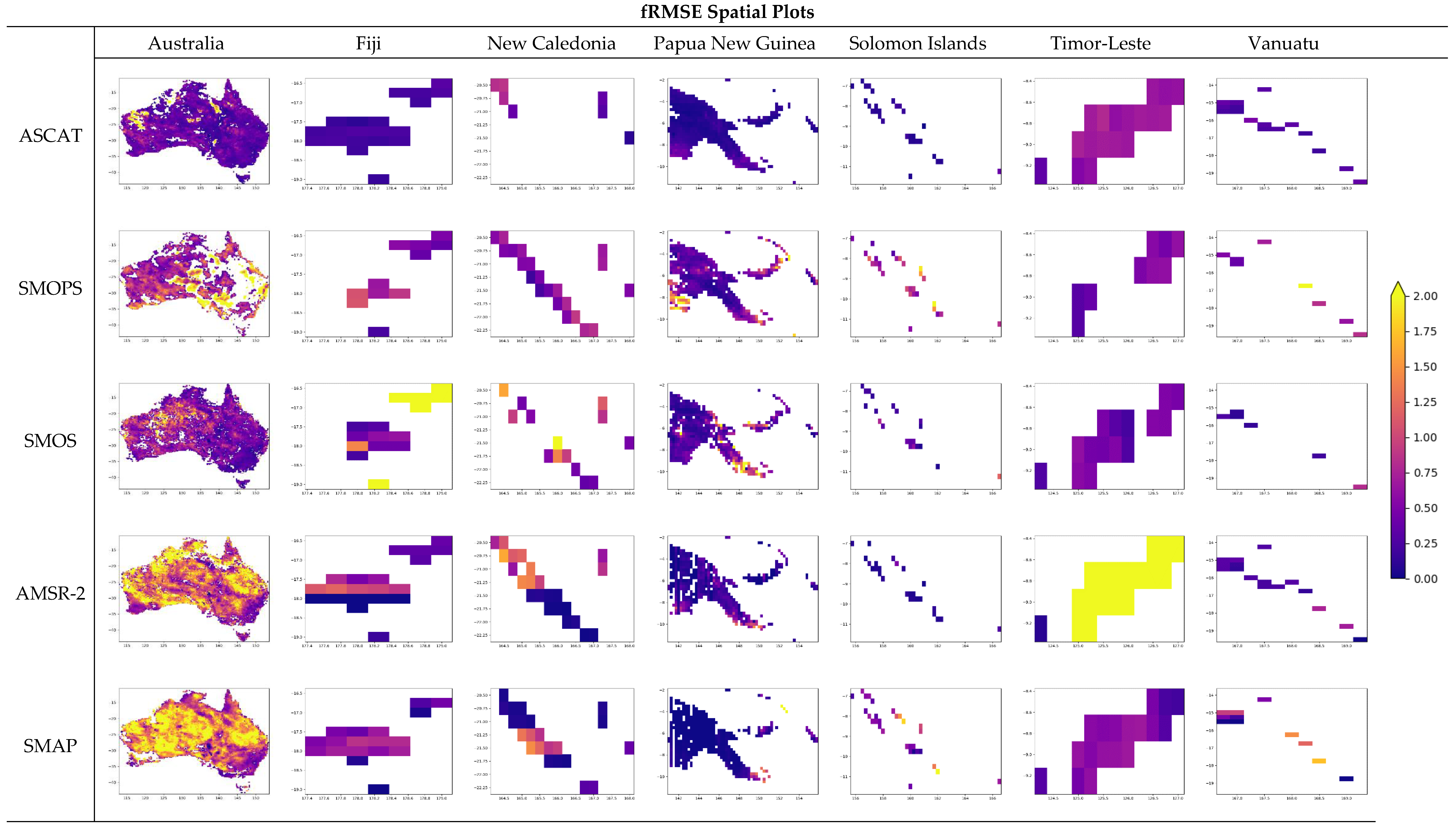
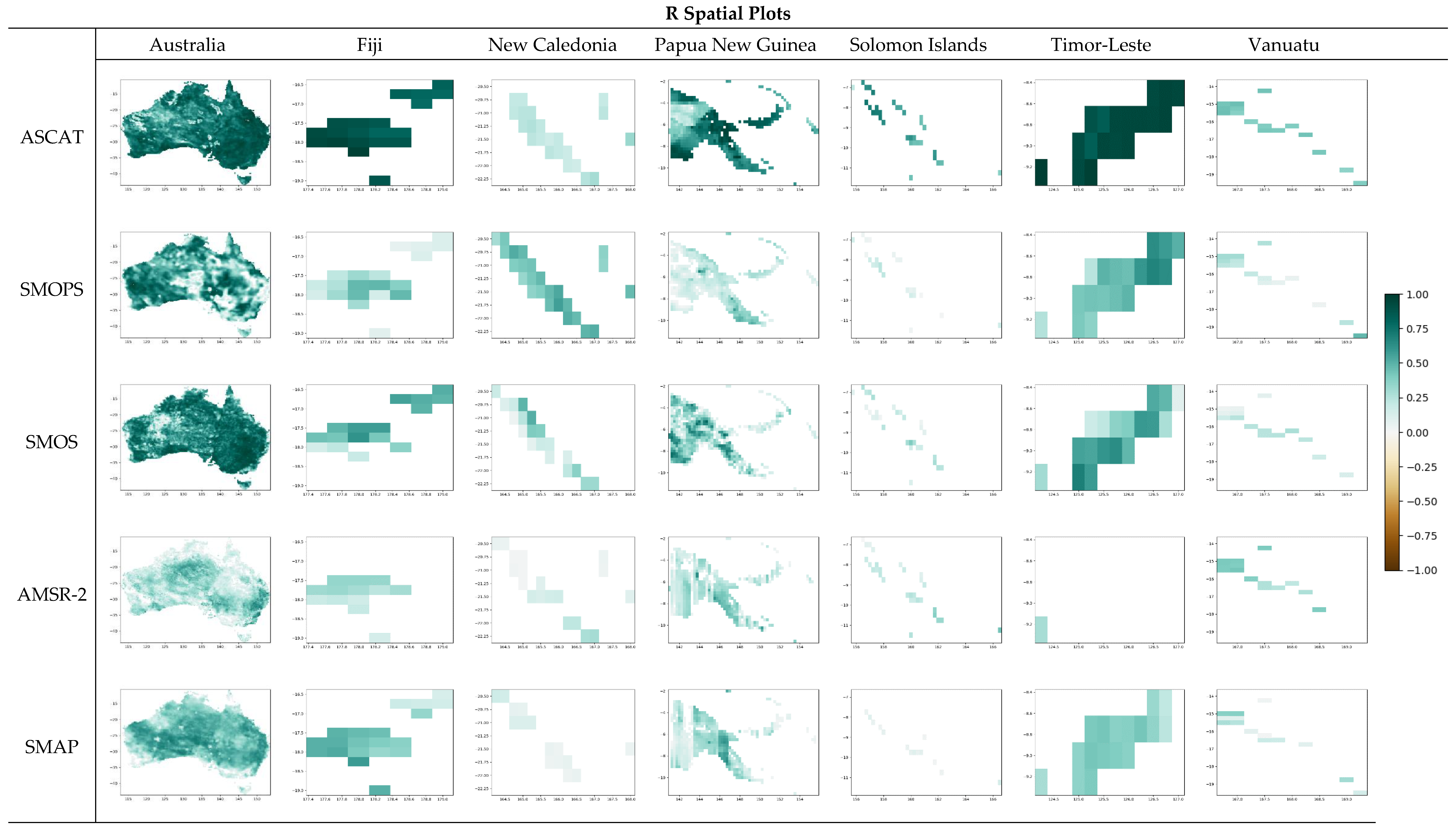
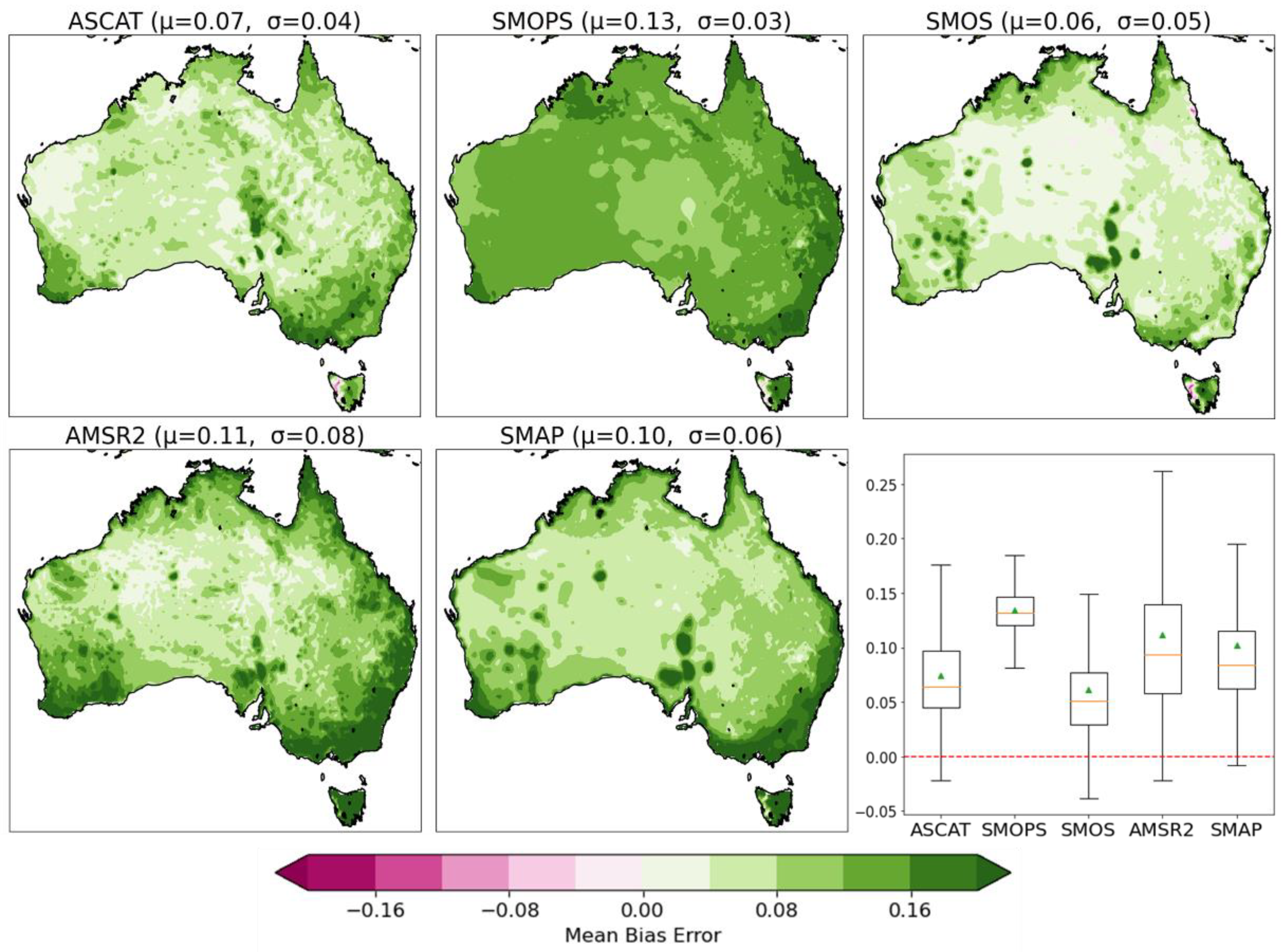
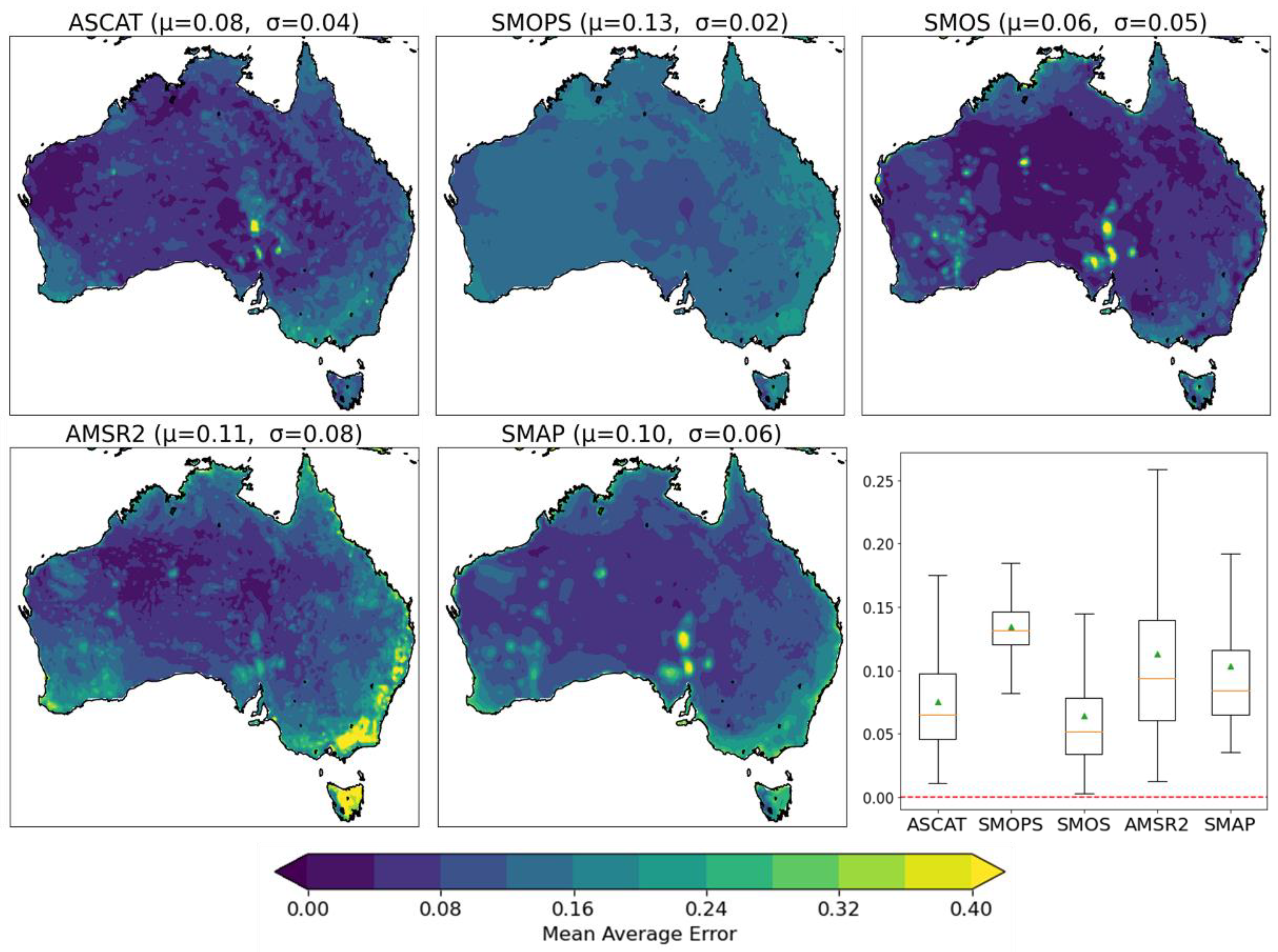
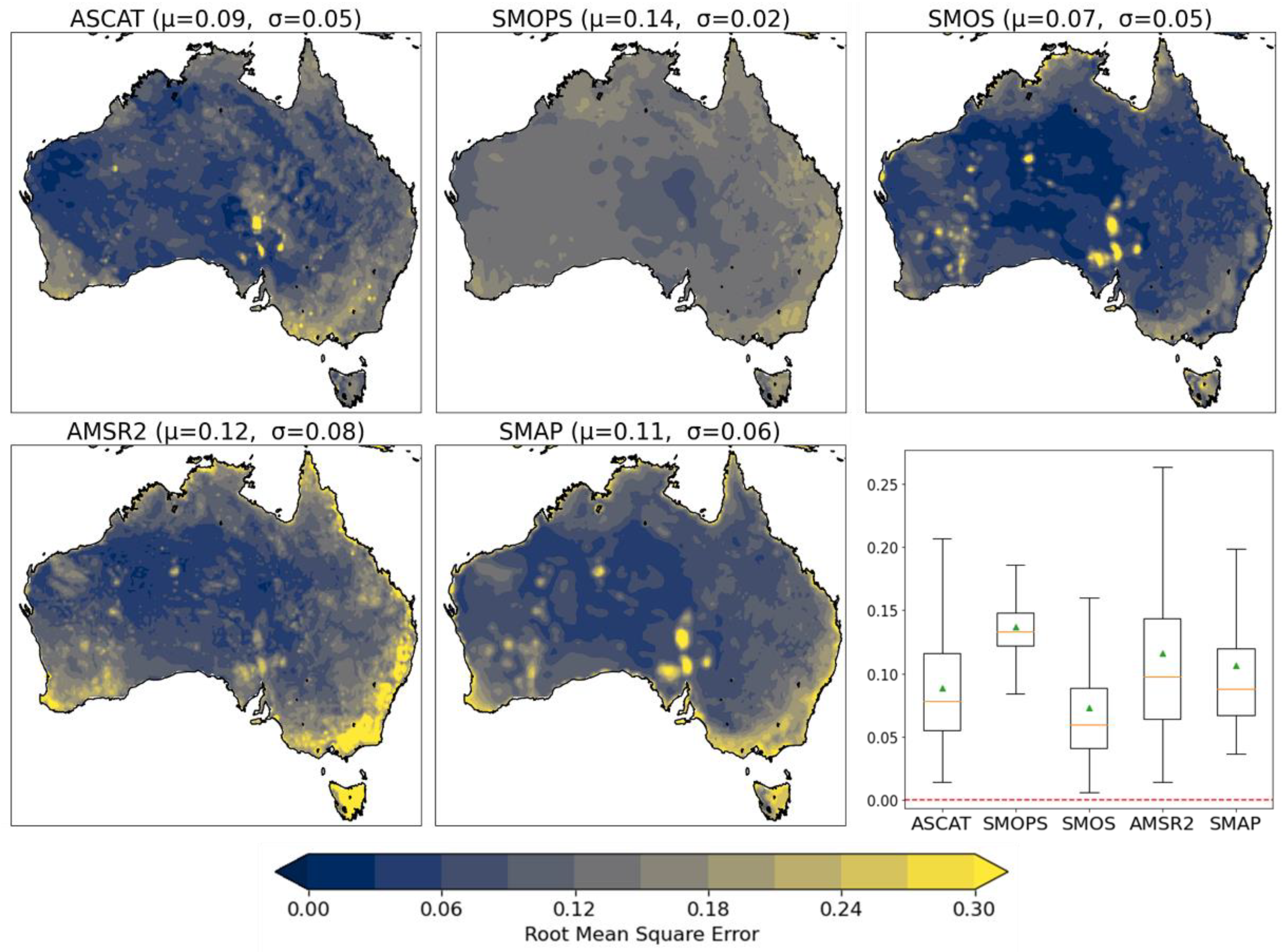
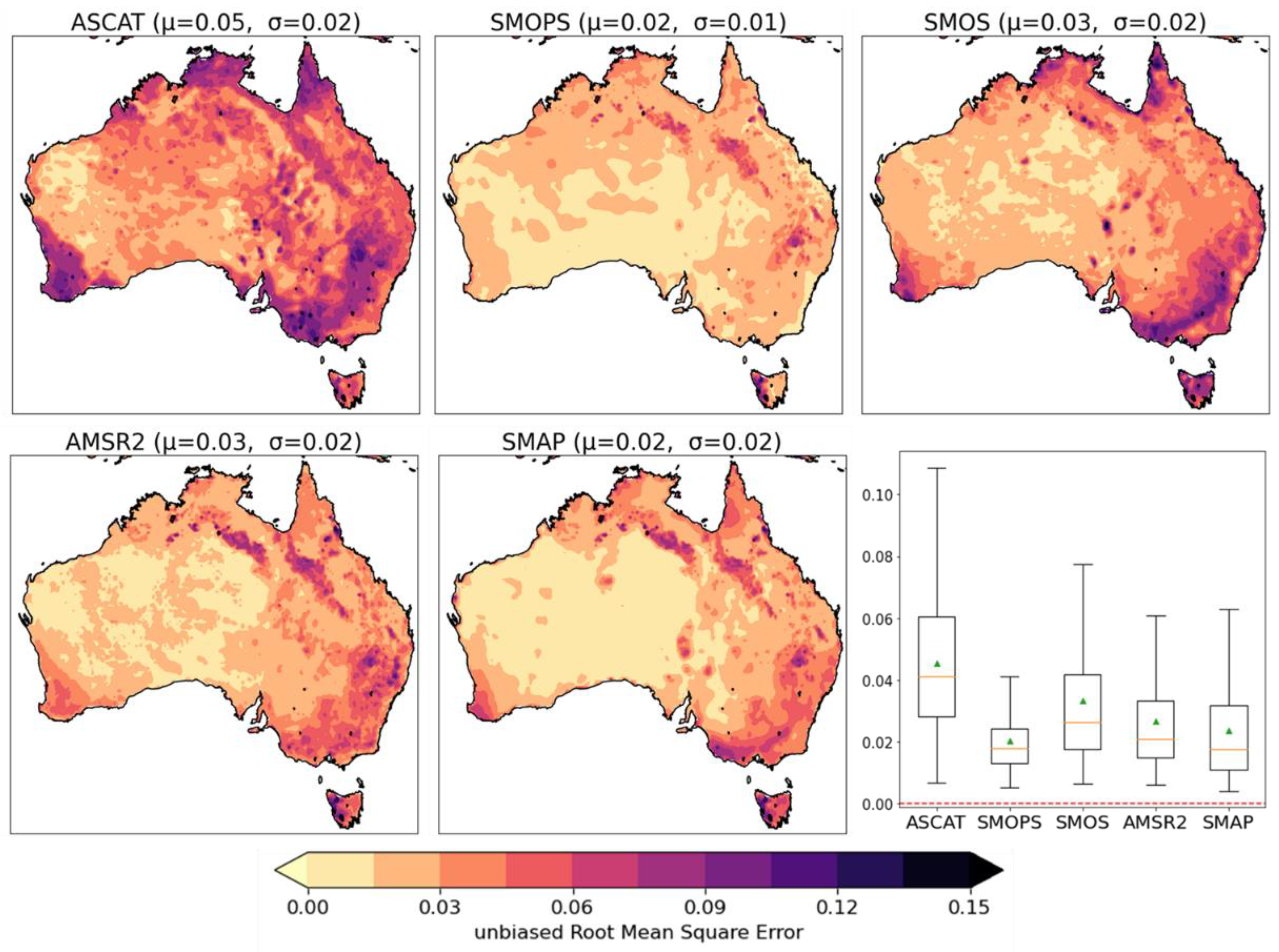
3.2. Gridded Analysis

| ASCAT | SMOPS | SMOS | AMSR-2 | SMAP | |
|---|---|---|---|---|---|
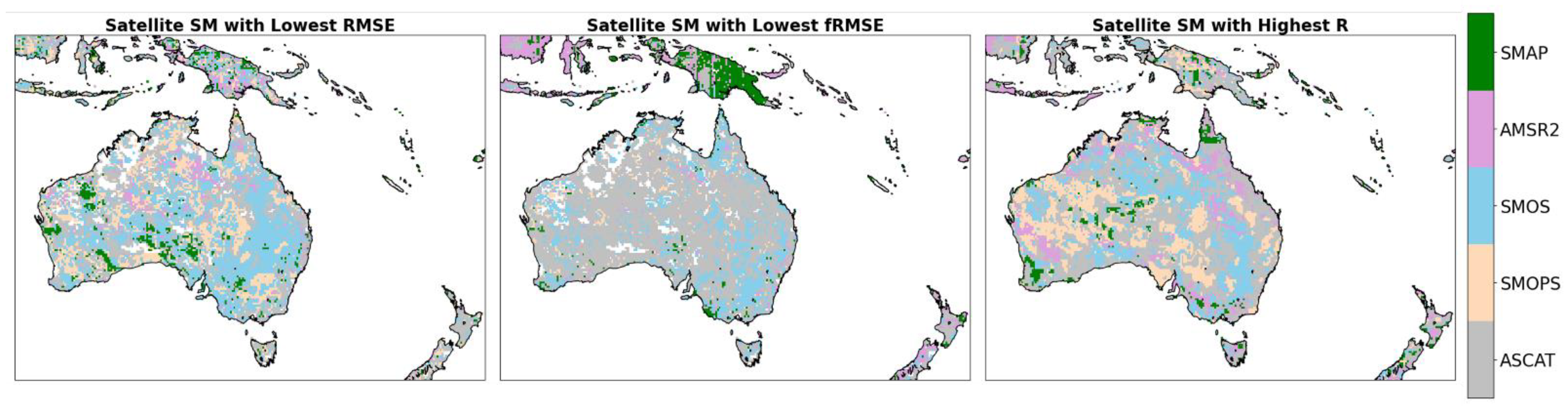
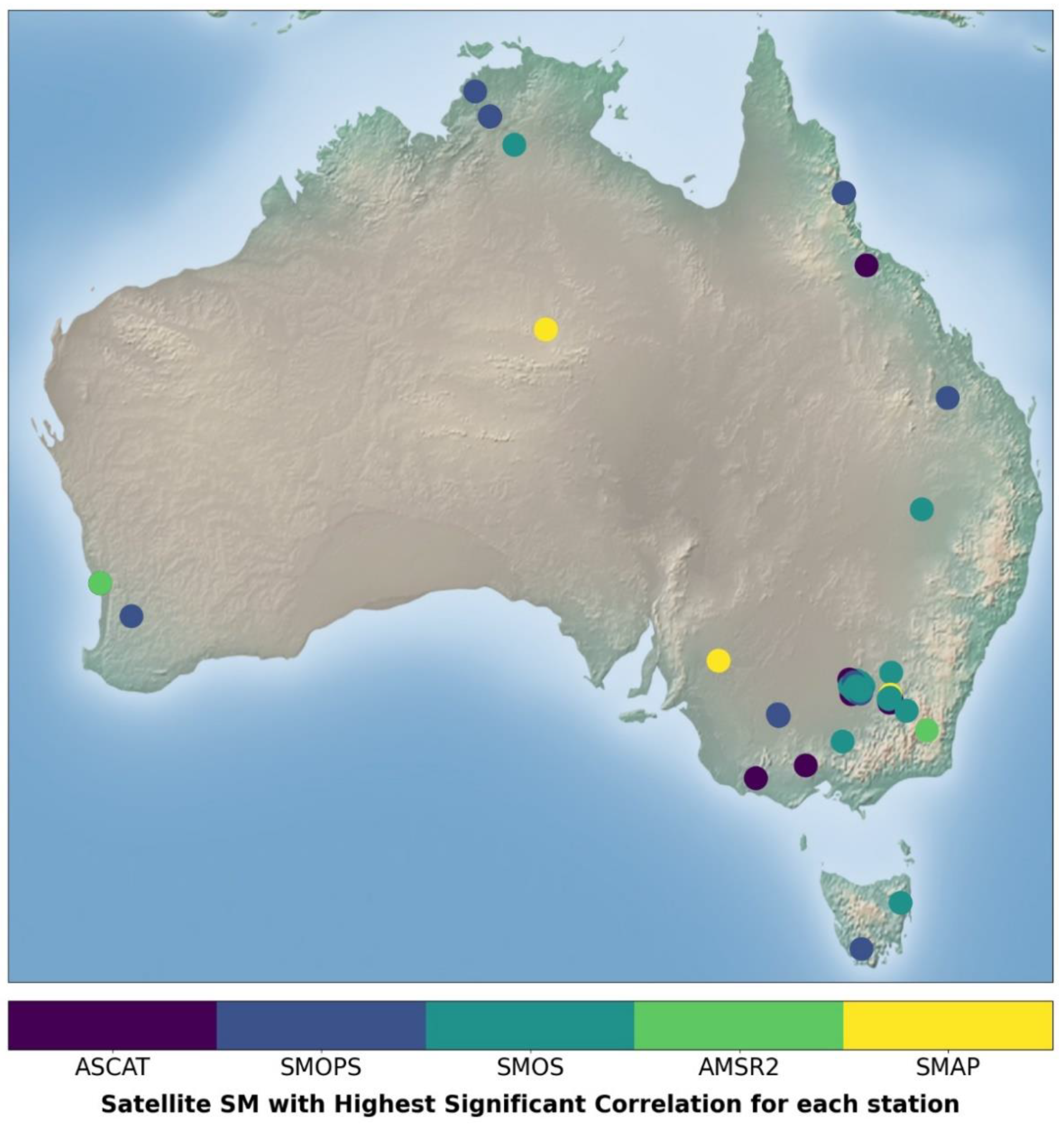
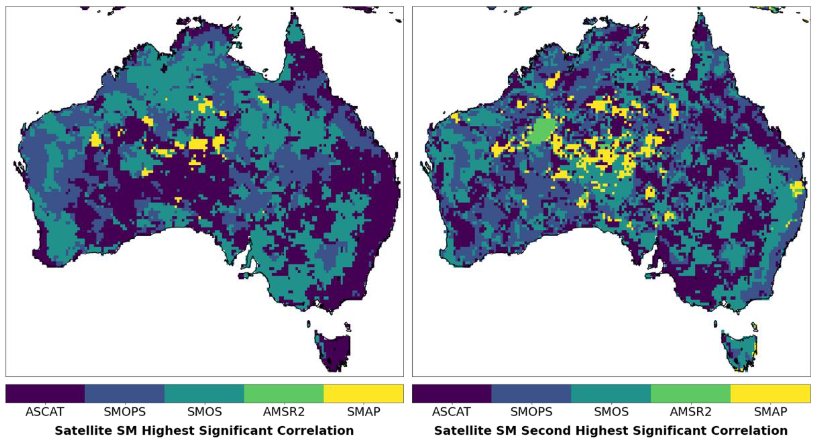
| % Highest Significant Correlation | 38.36 | 24.79 | 35.18 | 0.02 | 1.65 |
| % Second Highest Significant Correlation | 32.07 | 29.44 | 32.17 | 1.08 | 5.24 |
3.3. Triple Collocation Analysis
3.4. Case Study: Agrometeorological Drought in PNG
4. Discussion
4.1. Varying Dataset Performance
4.2. Performance along the Southeast Coast
4.3. Drought Monitoring and Early Warning Implications
5. Conclusions
Author Contributions
Funding
Data Availability Statement
Conflicts of Interest
Appendix A. Station Metadata
| Probe Type Key: (⊙) CS615/CS616, (❖), CS650, (★) Hydraprobe, (▪) Cosmic Ray Probe | |||||||
| CosmOz | |||||||
| Station | Latitude | Longitude | Elevation (m) | Station | Latitude | Longitude | Elevation (m) |
| Station 2 (Daly) ▪ | −14.16 | 131.39 | 75 | Station 11 (Yanco) ▪ | −35.01 | 146.3 | 124 |
| Station 3 (Gnangara) ▪ | −31.38 | 115.71 | 50 | Station 15 (Hamilton) ▪ | −37.8288 | 142.0895 | 199 |
| Station 6 (Robson) ▪ | −17.12 | 145.63 | 715 | Station 18 (Bishes) ▪ | −35.7694 | 142.9726 | 94 |
| Station 7 (Temora) ▪ | −34.4 | 147.53 | 294 | Station 19 (Bennets) ▪ | −35.8258 | 143.0039 | 98 |
| Station 8 (Tullochgorum) ▪ | −41.67 | 147.91 | 285 | Station 21 (Bullawarrie) ▪ | −28.8093 | 148.7651 | 166 |
| Station 9 (Tumbarumba) ▪ | −35.656 | 148.152 | 1200 | Station 22 (Scotts Peak) ▪ | −43.0418 | 146.337 | 305 |
| Station 10 (Weany) ▪ | −19.88 | 146.54 | 287 | Station 23 (Brigalow C3) ▪ | −24.812 | 149.8012 | 165 |
| OzNet | |||||||
| Station | Latitude | Longitude | Elevation (m) | Station | Latitude | Longitude | Elevation (m) |
| m1 ⊙ | −36.293 | 148.970567 | 937 | YA9 ★ | −34.7414 | 146.15364 | 133 |
| m2 ⊙ | −35.3088 | 149.2 | 639 | YB1 ★ | −34.9412 | 146.27654 | 123 |
| m3 ⊙ | −34.6299 | 148.0365 | 333 | YB3 ★ | −34.9427 | 146.34015 | 126 |
| m4 ⊙ | −33.9383 | 147.196183 | 258 | YB5a ★ | −34.9653 | 146.30262 | 123 |
| m5 ⊙ | −34.6584 | 143.54863 | 62 | YB5b ★ | −34.9634 | 146.31843 | 123 |
| m6 ⊙ | −34.5471 | 144.867 | 90 | YB5d ★ | −34.9848 | 146.29299 | 122 |
| m7 ⊙ | −34.249 | 146.07 | 137 | YB5e ★ | −34.9797 | 146.32052 | 121 |
| y1 ⊙★ | −34.6289 | 145.84895 | 120 | YB7a ★ | −34.9885 | 146.26941 | 126 |
| y2 ⊙★ | −34.6548 | 146.11028 | 130 | YB7c ★ | −34.9984 | 146.27852 | 125 |
| y3 ⊙ | −34.6208 | 146.4239 | 144 | YB7d ★ | −35.005 | 146.2685 | 126 |
| y4 ⊙★ | −34.7194 | 146.02003 | 130 | YB7e ★ | −35.0077 | 146.28805 | 121 |
| y5 ⊙★ | −34.7284 | 146.29317 | 136 | YB9 ★ | −35.0022 | 146.33978 | 121 |
| y6 ⊙★ | −34.8426 | 145.86692 | 121 | a1 ⊙ | −35.4975 | 148.106488 | 772 |
| y7 ⊙★ | −34.8518 | 146.1153 | 128 | a2 ⊙ | −35.4283 | 148.131626 | 595 |
| y8 ⊙★ | −34.847 | 146.41398 | 149 | a3 ⊙ | −35.3997 | 148.101076 | 472 |
| y9 ⊙★ | −34.9678 | 146.01632 | 122 | a4 ⊙ | −35.3731 | 148.066082 | 457 |
| y10 ⊙★ | −35.0054 | 146.30988 | 119 | a5 ⊙ | −35.3602 | 148.085427 | 379 |
| y11 ⊙★ | −35.1098 | 145.93553 | 113 | k1 ⊙ | −35.4932 | 147.55912 | 437 |
| y12 ⊙★ | −35.0696 | 146.16893 | 120 | k2 ⊙ | −35.4353 | 147.53052 | 351 |
| y13 ⊙★ | −35.0903 | 146.30648 | 121 | k3 ⊙ | −35.4341 | 147.56893 | 318 |
| YA1 ★ | −34.6843 | 146.089695 | 131 | k4 ⊙ | −35.4269 | 147.6 | 296 |
| YA3 ★ | −34.6772 | 146.1397 | 132 | k5 ⊙ | −35.4193 | 147.60408 | 306 |
| YA4a ★ | −34.706 | 146.07937 | 131 | k6 ⊙★ | −35.3898 | 147.4572 | 317 |
| YA4b ★ | −34.7031 | 146.10529 | 132 | k7 ⊙★ | −35.3939 | 147.56618 | 259 |
| YA4c ★ | −34.7142 | 146.09425 | 132 | k8 ⊙★ | −35.3163 | 147.34387 | 326 |
| YA4d ★ | −34.7142 | 146.07506 | 130 | k9 ⊙★ | −35.3198 | 147.43633 | 241 |
| YA4e ★ | −34.7214 | 146.10297 | 132 | k10 ⊙★ | −35.324 | 147.5348 | 232 |
| YA5 ★ | −34.7129 | 146.127712 | 132 | k11 ⊙★ | −35.272 | 147.42902 | 327 |
| YA7a ★ | −34.7352 | 146.08197 | 130 | k12 ⊙★ | −35.2275 | 147.485 | 220 |
| YA7b ★ | −34.7378 | 146.09867 | 131 | k13 ⊙★ | −35.2389 | 147.5333 | 261 |
| YA7d ★ | −34.7544 | 146.07777 | 129 | k14 ⊙★ | −35.1249 | 147.4974 | 184 |
| YA7e ★ | −34.7507 | 146.09493 | 131 | ||||
| OzFlux | |||||||
| Station | Latitude | Longitude | Elevation (m) | Station | Latitude | Longitude | Elevation (m) |
| Adelaide River ⊙ | −13.0769 | 131.1178 | 90 | Loxton | −34.4704 | 140.6551 | - |
| Calperum ❖ | −34.0027 | 140.5875 | 65 | Otway ⊙ | −38.525 | 142.81 | 54 |
| Cape Tribulation ⊙ | −16.1032 | 145.4469 | 66 | Red Dirt Melon Farm | −14.5636 | 132.4776 | - |
| Cow Bay ⊙ | −16.2382 | 145.4272 | 86 | Ridgefield ★ | −32.5061 | 116.9668 | 330 |
| Cumberland Plain | −33.6153 | 150.7236 | 23 | Riggs Creek ⊙ | −36.656 | 145.576 | 152 |
| Daly Pasture ⊙ | −17.1507 | 133.3502 | 70 | Robson Creek ⊙ | −17.1175 | 145.6301 | 710 |
| Daly Uncleared ⊙ | −14.1592 | 131.3881 | 110 | Ti Tree East ⊙ | −22.287 | 133.64 | 553 |
| Dry River ⊙ | −15.2588 | 132.3706 | 175 | Tumbarumba | −35.6566 | 148.1516 | 1200 |
| Emerald | −23.8587 | 148.4746 | - | Wallaby Creek ⊙ | −37.4259 | 145.1878 | 600 |
| Fogg Dam ⊙ | −12.5452 | 131.3072 | 4 | Warra ⊙ | −43.095 | 146.6545 | 100 |
| Gingin ⊙ | −31.3764 | 115.7138 | 51 | Whroo ⊙ | −36.6732 | 145.0294 | 165 |
| Great Western Woodlands ⊙ | −30.1914 | 120.6542 | 500 | Wombat State Forest ⊙ | −37.4222 | 144.0944 | 713 |
| Howard Springs ⊙ | −12.4952 | 131.1501 | 64 | Yanco | −34.9878 | 146.2908 | - |
| Litchfield ⊙ | −13.179 | 130.7945 | - | ||||
Appendix B. Detailed TC Results
References
- Heimann, M.; Reichstein, M. Terrestrial Ecosystem Carbon Dynamics and Climate Feedbacks. Nature 2008, 451, 289–292. [Google Scholar] [CrossRef] [PubMed]
- Babaeian, E.; Sadeghi, M.; Jones, S.B.; Montzka, C.; Vereecken, H.; Tuller, M. Ground, Proximal, and Satellite Remote Sensing of Soil Moisture. Rev. Geophys. 2019, 57, 530–616. [Google Scholar] [CrossRef]
- Mohanty, B.P.; Cosh, M.H.; Lakshmi, V.; Montzka, C. Soil Moisture Remote Sensing: State-of-the-Science. Vadose Zone J. 2017, 16, 1–9. [Google Scholar] [CrossRef]
- Wang, L.; Qu, J.J. Satellite Remote Sensing Applications for Surface Soil Moisture Monitoring: A Review. Front. Earth Sci. China 2009, 3, 237–247. [Google Scholar] [CrossRef]
- Gruber, A.; Dorigo, W.A.; Zwieback, S.; Xaver, A.; Wagner, W. Characterizing Coarse-Scale Representativeness of in Situ Soil Moisture Measurements from the International Soil Moisture Network. Vadose Zone J. 2013, 12, 1–16. [Google Scholar] [CrossRef]
- Kim, S.; Zhang, R.; Pham, H.; Sharma, A. A Review of Satellite-Derived Soil Moisture and Its Usage for Flood Estimation. Remote Sens. Earth Syst. Sci. 2019, 2, 225–246. [Google Scholar] [CrossRef]
- Jackson, T.J.; Le Vine, D.M.; Hsu, A.Y.; Oldak, A.; Starks, P.J.; Swift, C.T.; Isham, J.D.; Haken, M. Soil Moisture Mapping at Regional Scales Using Microwave Radiometry: The Southern Great Plains Hydrology Experiment. IEEE Trans. Geosci. Remote Sens. 1999, 37, 2136–2151. [Google Scholar] [CrossRef]
- Kuleshov, Y.; Kurino, T.; Kubota, T.; Tashima, T.; Xie, P. WMO Space-Based Weather and Climate Extremes Monitoring Demonstration Project (SEMDP): First Outcomes of Regional Cooperation on Drought and Heavy Precipitation Monitoring for Australia and Southeast Asia. In Rainfall—Extremes, Distribution and Properties; IntechOpen: London, UK, 2019; ISBN 978-1-78984-734-5. [Google Scholar]
- McGree, S.; Schreider, S.; Kuleshov, Y. Trends and Variability in Droughts in the Pacific Islands and Northeast Australia. J. Clim. 2016, 29, 8377–8397. [Google Scholar] [CrossRef]
- Mcleod, E.; Bruton-Adams, M.; Förster, J.; Franco, C.; Gaines, G.; Gorong, B.; James, R.; Posing-Kulwaum, G.; Tara, M.; Terk, E. Lessons from the Pacific Islands—Adapting to Climate Change by Supporting Social and Ecological Resilience. Front. Mar. Sci. 2019, 6, 289. [Google Scholar] [CrossRef]
- Luchetti, N.T.; Sutton, J.R.P.; Wright, E.E.; Kruk, M.C.; Marra, J.J. When El Niño Rages: How Satellite Data Can Help Water-Stressed Islands. Bull. Am. Meteorol. Soc. 2016, 97, 2249–2255. [Google Scholar] [CrossRef]
- Jacka, J.K. In the Time of Frost: El Niño and the Political Ecology of Vulnerability in Papua New Guinea. Anthropol. Forum 2020, 30, 141–156. [Google Scholar] [CrossRef]
- Murphy, B.F.; Power, S.B.; McGree, S. The Varied Impacts of El Niño–Southern Oscillation on Pacific Island Climates. J. Clim. 2014, 27, 4015–4036. [Google Scholar] [CrossRef]
- Intergovernmental Panel on Climate Change (IPCC); Masson-Delmotte, V.; Zhai, P.; Pirani, A.; Connors, S.L.; Péan, C.; Berger, S.; Caud, N.; Chen, Y.; Goldfarb, L.; et al. Climate Change 2021: The Physical Science Basis. Contribution of Working Group I to the Sixth Assessment Report of the Intergovernmental Panel on Climate Change; IPCC: Geneva, Switzerland, 2021. [Google Scholar]
- Chua, Z.-W.; Kuleshov, Y.; Watkins, A.B. Drought Detection over Papua New Guinea Using Satellite-Derived Products. Remote Sens. 2020, 12, 3859. [Google Scholar] [CrossRef]
- Wild, A.; Chua, Z.-W.; Kuleshov, Y. Evaluation of Satellite Precipitation Estimates over the South West Pacific Region. Remote Sens. 2021, 13, 3929. [Google Scholar] [CrossRef]
- Wimhurst, J.J.; Greene, J.S. Updated Analysis of Gauge-Based Rainfall Patterns over the Western Tropical Pacific Ocean. Weather Clim. Extrem. 2021, 32, 100319. [Google Scholar] [CrossRef]
- Pariyar, S.K.; Keenlyside, N.; Sorteberg, A.; Spengler, T.; Chandra Bhatt, B.; Ogawa, F. Factors Affecting Extreme Rainfall Events in the South Pacific. Weather Clim. Extrem. 2020, 29, 100262. [Google Scholar] [CrossRef]
- Wagner, W.; Lemoine, G.; Rott, H. A Method for Estimating Soil Moisture from ERS Scatterometer and Soil Data. Remote Sens. Environ. 1999, 70, 191–207. [Google Scholar] [CrossRef]
- Kerr, Y.H.; Waldteufel, P.; Wigneron, J.P.; Delwart, S.; Cabot, F.; Boutin, J.; Escorihuela, M.J.; Font, J.; Reul, N.; Gruhier, C.; et al. The SMOS L: New Tool for Monitoring Key Elements Ofthe Global Water Cycle. Proc. IEEE 2010, 98, 666–687. [Google Scholar] [CrossRef]
- Liu, J.; Zhan, X.; Hain, C.; Yin, J.; Fang, L.; Li, Z.; Zhao, L. NOAA Soil Moisture Operational Product System (SMOPS) and Its Validations. In Proceedings of the 2016 IEEE International Geoscience and Remote Sensing Symposium (IGARSS), Beijing, China, 10–15 July 2016; pp. 3477–3480. [Google Scholar]
- De Jeu, R.; Owe, M.; GES DISC; Teng, B. AMSR2/GCOM-W1 Surface Soil Moisture (LPRM) L3 1 Day 10 Km × 10 Km Descending V001; Goddard Earth Sciences Data and Information Services Center: Greenbelt, MD, USA, 2014.
- O’Neill, P.E.; Chan, S.; Njoku, E.G.; Jackson, T.; Bindlish, R.; Chaubell, J. SMAP L3 Radiometer Global Daily 36 km EASE-Grid Soil Moisture; Version 7; NASA National Snow and Ice Data Center Distributed Active Archive Center: Boulder, CO, USA, 2020; pp. 1–28.
- Frost, A.J.; Ramchurn, A.; Smith, A. The Australian Landscape Water Balance Model (AWRA-L v6); Technical Description of the Australian Water Resources Assessment Landscape Model Version 6; Bureau of Meteorology Technical Report; Bureau of Meteorology: Melbourne, Australia, 2018.
- Rodell, M.; Houser, P.R.; Jambor, U.; Gottschalck, J.; Mitchell, K.; Meng, C.J.; Arsenault, K.; Cosgrove, B.; Radakovich, J.; Bosilovich, M.; et al. The Global Land Data Assimilation System. Bull. Am. Meteorol. Soc. 2004, 85, 381–394. [Google Scholar] [CrossRef]
- Muñoz Sabater, J. ERA5-Land Monthly Averaged Data from 1950 to 1980. Available online: https://cds.climate.copernicus.eu/cdsapp#!/dataset/reanalysis-era5-land-monthly-means?tab=overview (accessed on 6 June 2022).
- Smith, A.B.; Walker, J.P.; Western, A.W.; Young, R.I.; Ellett, K.M.; Pipunic, R.C.; Grayson, R.B.; Siriwardena, L.; Chiew, F.H.S.; Richter, H. The Murrumbidgee Soil Moisture Monitoring Network Data Set. Water Resour. Res. 2012, 48, W07701. [Google Scholar] [CrossRef]
- Hawdon, A.; McJannet, D.; Wallace, J. Calibration and Correction Procedures for Cosmic-Ray Neutron Soil Moisture Probes Located across Australia. Water Resour. Res. 2014, 50, 5029–5043. [Google Scholar] [CrossRef]
- Beringer, J.; Hutley, L.B.; McHugh, I.; Arndt, S.K.; Campbell, D.; Cleugh, H.A.; Cleverly, J.; De Dios, V.R.; Eamus, D.; Evans, B.; et al. An Introduction to the Australian and New Zealand Flux Tower Network—OzFlux. Biogeosciences 2016, 13, 5895–5916. [Google Scholar] [CrossRef]
- Yuan, X.; Ma, Z.; Pan, M.; Shi, C. Microwave Remote Sensing of Short-Term Droughts during Crop Growing Seasons. Geophys. Res. Lett. 2015, 42, 4394–4401. [Google Scholar] [CrossRef]
- Integrated Climate Data Center (ICDC). Globally Gridded Monthly Mean ASCAT Soil Moisture Maps. 2022. Available online: https://www.fdr.uni-hamburg.de/record/10196 (accessed on 6 June 2022).
- Wu, X.; Lu, G.; Wu, Z.; He, H.; Scanlon, T.; Dorigo, W. Triple Collocation-Based Assessment of Satellite Soil Moisture Products with in Situ Measurements in China: Understanding the Error Sources. Remote Sens. 2020, 12, 2275. [Google Scholar] [CrossRef]
- Molero, B.; Merlin, O.; Malbéteau, Y.; Al Bitar, A.; Cabot, F.; Stefan, V.; Kerr, Y.; Bacon, S.; Cosh, M.H.; Bindlish, R.; et al. SMOS Disaggregated Soil Moisture Product at 1 Km Resolution: Processor Overview and First Validation Results. Remote Sens. Environ. 2016, 180, 361–376. [Google Scholar] [CrossRef]
- Zhan, X.; Liu, J.; Zhao, L. Soil Moisture Operational Product System (SMOPS): Algorithm Theoretical Basis Document—Version 4.0; NOAA NESDIS STAR: Suitland, MD, USA, 2016.
- Pablos, M.; González-Haro, C.; Piles, M.; BEC Team. BEC SMOS Soil Moisture Products Description (V. 1.0). 2020. Available online: https://bec.icm.csic.es/data/available-products/#SoilMoisture (accessed on 6 June 2022).
- Owe, M.; de Jeu, R.; Holmes, T. Multisensor Historical Climatology of Satellite-Derived Global Land Surface Moisture. J. Geophys. Res. Earth Surf. 2008, 113. [Google Scholar] [CrossRef]
- Wang, Y.; Yang, J.; Chen, Y.; De Maeyer, P.; Li, Z.; Duan, W. Detecting the Causal Effect of Soil Moisture on Precipitation Using Convergent Cross Mapping. Sci. Rep. 2018, 8, 12171. [Google Scholar] [CrossRef]
- Mousa, B.G.; Shu, H. Spatial Evaluation and Assimilation of SMAP, SMOS, and ASCAT Satellite Soil Moisture Products Over Africa Using Statistical Techniques. Earth Sp. Sci. 2020, 7, e2019EA000841. [Google Scholar] [CrossRef]
- Bureau of Meteorology Climate Classification Maps (Köppen—Major Classes). Available online: http://www.bom.gov.au/jsp/ncc/climate_averages/climate-classifications/index.jsp?maptype=kpngrp#maps (accessed on 6 June 2022).
- Holgate, C.M.; De Jeu, R.A.M.; van Dijk, A.I.J.M.; Liu, Y.Y.; Renzullo, L.J.; Vinodkumar; Dharssi, I.; Parinussa, R.M.; Van Der Schalie, R.; Gevaert, A.; et al. Comparison of Remotely Sensed and Modelled Soil Moisture Data Sets across Australia. Remote Sens. Environ. 2016, 186, 479–500. [Google Scholar] [CrossRef]
- Scipal, K.; Holmes, T.; De Jeu, R.; Naeimi, V.; Wagner, W. A Possible Solution for the Problem of Estimating the Error Structure of Global Soil Moisture Data Sets. Geophys. Res. Lett. 2008, 35. [Google Scholar] [CrossRef]
- Stoffelen, A. Toward the True Near-Surface Wind Speed: Error Modeling and Calibration Using Triple Collocation. J. Geophys. Res. Ocean. 1998, 103, 7755–7766. [Google Scholar] [CrossRef]
- Draper, C.; Reichle, R.; de Jeu, R.; Naeimi, V.; Parinussa, R.; Wagner, W. Estimating Root Mean Square Errors in Remotely Sensed Soil Moisture over Continental Scale Domains. Remote Sens. Environ. 2013, 137, 288–298. [Google Scholar] [CrossRef]
- McColl, K.A.; Vogelzang, J.; Konings, A.G.; Entekhabi, D.; Piles, M.; Stoffelen, A. Extended Triple Collocation: Estimating Errors and Correlation Coefficients with Respect to an Unknown Target. Geophys. Res. Lett. 2014, 41, 6229–6236. [Google Scholar] [CrossRef]
- Ming, W.; Ji, X.; Zhang, M.; Li, Y.; Liu, C.; Wang, Y.; Li, J. A Hybrid Triple Collocation-Deep Learning Approach for Improving Soil Moisture Estimation from Satellite and Model-Based Data. Remote Sens. 2022, 14, 1744. [Google Scholar] [CrossRef]
- NOAA National Geophysical Data Center. ETOPO1 1 Arc-Minute Global Relief Model; NOAA National Centers for Environmental Information: Asheville, NC, USA, 2009. [CrossRef]
- National Aeronautics and Space Administration (NASA). How Can I Obtain Volumetric Soil Moisture [M3 m−3] from the LDAS Data? Available online: https://ldas.gsfc.nasa.gov/faq/LDAS#:~:text=To convert to units of,%5Bkg m-3%5D (accessed on 6 June 2022).
- McKee, T.B. Drought Monitoring with Multiple Time Scales. In Proceedings of the 9th Conference on Applied Climatology, Boston, MA, USA, 15–20 January 1995. [Google Scholar]
- Kogan, F.N. Droughts of the Late 1980s in the United States as Derived from NOAA Polar-Orbiting Satellite Data. Bull.-Am. Meteorol. Soc. 1995, 76, 655–668. [Google Scholar] [CrossRef]
- Schmidt, E.; Gilbert, R.; Holtemeyer, B.; Mahrt, K. Poverty Analysis in the Lowlands of Papua New Guinea Underscores Climate Vulnerability and Need for Income Flexibility. Aust. J. Agric. Resour. Econ. 2021, 65, 171–191. [Google Scholar] [CrossRef]
- Link, M.; Drusch, M.; Scipal, K. Soil Moisture Information Content in SMOS, SMAP, AMSR2, and ASCAT Level-1 Data over Selected in Situ Sites. IEEE Geosci. Remote Sens. Lett. 2020, 17, 1213–1217. [Google Scholar] [CrossRef]
- Kerr, Y.H.; Waldteufel, P.; Richaume, P.; Wigneron, J.P.; Ferrazzoli, P.; Mahmoodi, A.; Al Bitar, A.; Cabot, F.; Gruhier, C.; Juglea, S.E.; et al. The SMOS Soil Moisture Retrieval Algorithm. IEEE Trans. Geosci. Remote Sens. 2012, 50, 1384–1403. [Google Scholar] [CrossRef]
- Montzka, C.; Bogena, H.R.; Zreda, M.; Monerris, A.; Morrison, R.; Muddu, S.; Vereecken, H. Validation of Spaceborne and Modelled Surface Soil Moisture Products with Cosmic-Ray Neutron Probes. Remote Sens. 2017, 9, 103. [Google Scholar] [CrossRef]
- Su, C.H.; Zhang, J.; Gruber, A.; Parinussa, R.; Ryu, D.; Crow, W.T.; Wagner, W. Error Decomposition of Nine Passive and Active Microwave Satellite Soil Moisture Data Sets over Australia. Remote Sens. Environ. 2016, 182, 128–140. [Google Scholar] [CrossRef]
- Albergel, C.; de Rosnay, P.; Gruhier, C.; Muñoz-Sabater, J.; Hasenauer, S.; Isaksen, L.; Kerr, Y.; Wagner, W. Evaluation of Remotely Sensed and Modelled Soil Moisture Products Using Global Ground-Based in Situ Observations. Remote Sens. Environ. 2012, 118, 215–226. [Google Scholar] [CrossRef]
- Wagner, W.; Hahn, S.; Kidd, R.; Melzer, T.; Bartalis, Z.; Hasenauer, S.; Figa-Saldaña, J.; De Rosnay, P.; Jann, A.; Schneider, S.; et al. The ASCAT Soil Moisture Product: A Review of Its Specifications, Validation Results, and Emerging Applications. Meteorol. Z. 2013, 22, 5–33. [Google Scholar] [CrossRef]
- Frost, A.J.; Shokri, A. The Australian Landscape Water Balance Model (AWRA-L v7); Technical Description of the Australian Water Resources Assessment Landscape Model Version 7; Bureau of Meteorology: Melbourne, Australia, 2021.
- Beck, H.E.; Pan, M.; Miralles, D.G.; Reichle, R.H.; Dorigo, W.A.; Hahn, S.; Sheffield, J.; Karthikeyan, L.; Balsamo, G.; Parinussa, R.M.; et al. Evaluation of 18 Satellite—And Model-Based Soil Moisture Products Using in Situ Measurements from 826 Sensors. Hydrol. Earth Syst. Sci. 2021, 25, 17–40. [Google Scholar] [CrossRef]
- Bhardwaj, J.; Kuleshov, Y.; Chua, Z.-W.; Watkins, A.B.; Choy, S.; Sun, Q. Building Capacity for a User-Centred Integrated Early Warning System for Drought in Papua New Guinea. Remote Sens. 2021, 13, 3307. [Google Scholar] [CrossRef]
- Ilan, K.; Jessica, M.; Gaillard, J.C. Indigenous Knowledge and Disaster Risk Reduction. Geography 2012, 97, 12–21. [Google Scholar] [CrossRef]
- Granderson, A.A. The Role of Traditional Knowledge in Building Adaptive Capacity for Climate Change: Perspectives from Vanuatu. Weather. Clim. Soc. 2017, 9, 545–561. [Google Scholar] [CrossRef]


| Dataset [Reference] | Sensor/Model/Probe Type (Frequency, GHz) | Sponsor | Sampling Depth (cm) | Resolution/ Nstations | Temporal Coverage | Unit | |
|---|---|---|---|---|---|---|---|
| Satellite | ASCAT [19] | Active, C band (5.3) | EUMETSAT | 0.5–2 | 12.5/25/50 km | 2007-now | % saturation |
| SMOS [20] | Passive, L band (1.4) | ESA | 0–5 | 15/25 km | 2010-now | m3/m3 | |
| SMOPS [21] | merged product | NASA | 1–5 | 0.25 deg | 2015-now | m3/m3 | |
| ASMR-2 [22] | Passive, C (6.9/7.3) X (10.7) | NASA/JAXA | 0–0.5 | 0.1/0.25 deg | 2012-now | m3/m3 | |
| SMAP [23] | Active/Passive, L band (1.26/1.41) | NASA | 0–5 | 3/9/36 km | 2015-now | m3/m3 | |
| Modelled | AWRA-L [24] | Open loop (no data assimilation) | BoM | 0–10 | 0.05 deg | 1911-now | m3/m3 |
| GLDAS [25] | Global Water Balance Model | NASA | 0–10 | 0.25 deg | 1948–2020 | kg/m2 | |
| ERA-5 Land [26] | ECMWF Reanalysis | ECMWF/Copernicus | 0–7 | 0.1 deg | 1950-now | m3/m3 | |
| In-Situ | OzNet [27] | Reflectometers/Hydraprobes | Monash/Melbourne | 0–5, 0–8, 0–10, 0–30, 30–60, 60–90 | 62 | 2001-now | m3/m3 |
| CosmOz [28] | Cosmic Neutron Ray | CSIRO/TERN | 14 | 2010-now | m3/m3 | ||
| OzFlux [29] | Reflectometers/Hydraprobes | Monash | 23 | 2002-now | m3/m3 | ||
| Metric and Analytical Purpose | Equation | Range | Perfect Value | Unit |
|---|---|---|---|---|
| MBE Mean systematic difference between estimated SM and ‘true’ SM. | (−∞, ∞) | 0 | m3/m3 | |
| MAE Mean absolute difference between estimated SM and ‘true’ SM. | [0, ∞) | 0 | m3/m3 | |
| RMSE Spread or standard deviation of errors for estimated SM. | [0, ∞) | 0 | m3/m3 | |
| ubRMSE Spread or standard deviation of random error for estimated SM after systematic differences are removed. | [0, ∞) | 0 | m3/m3 | |
| R A statistical metric that measures the strength and direction of correlation between estimated SM and ‘true’ SM. | [−1, 1] | 1 | unitless |
Publisher’s Note: MDPI stays neutral with regard to jurisdictional claims in published maps and institutional affiliations. |
© 2022 by the authors. Licensee MDPI, Basel, Switzerland. This article is an open access article distributed under the terms and conditions of the Creative Commons Attribution (CC BY) license (https://creativecommons.org/licenses/by/4.0/).
Share and Cite
Bhardwaj, J.; Kuleshov, Y.; Chua, Z.-W.; Watkins, A.B.; Choy, S.; Sun, Q. Evaluating Satellite Soil Moisture Datasets for Drought Monitoring in Australia and the South-West Pacific. Remote Sens. 2022, 14, 3971. https://doi.org/10.3390/rs14163971
Bhardwaj J, Kuleshov Y, Chua Z-W, Watkins AB, Choy S, Sun Q. Evaluating Satellite Soil Moisture Datasets for Drought Monitoring in Australia and the South-West Pacific. Remote Sensing. 2022; 14(16):3971. https://doi.org/10.3390/rs14163971
Chicago/Turabian StyleBhardwaj, Jessica, Yuriy Kuleshov, Zhi-Weng Chua, Andrew B. Watkins, Suelynn Choy, and Qian (Chayn) Sun. 2022. "Evaluating Satellite Soil Moisture Datasets for Drought Monitoring in Australia and the South-West Pacific" Remote Sensing 14, no. 16: 3971. https://doi.org/10.3390/rs14163971
APA StyleBhardwaj, J., Kuleshov, Y., Chua, Z.-W., Watkins, A. B., Choy, S., & Sun, Q. (2022). Evaluating Satellite Soil Moisture Datasets for Drought Monitoring in Australia and the South-West Pacific. Remote Sensing, 14(16), 3971. https://doi.org/10.3390/rs14163971