Multi-Scale Object Detection with the Pixel Attention Mechanism in a Complex Background

Abstract

The object detection task is usually affected by complex backgrounds. In this paper, a new image object detection method is proposed, which can perform multi-feature selection on multi-scale feature maps. By this method, a bidirectional multi-scale feature fusion network was designed to fuse semantic features and shallow features to improve the detection effects of small objects in complex backgrounds. When the shallow features are transferred to the top layer, a bottom-up path is added to reduce the number of network layers experienced by the feature fusion network, reducing the loss of shallow features. In addition, a multi-feature selection module based on the attention mechanism is used to minimize the interference of useless information in subsequent classification and regression, allowing the network to adaptively focus on appropriate information for classification or regression to improve detection accuracy. Because the traditional five-parameter regression method has severe boundary problems when predicting objects with large aspect ratios, the proposed network treats angle prediction as a classification task. The experimental results on the DOTA dataset, the self-made DOTA-GF dataset and the HRSC 2016 dataset show that, compared with several popular object detection algorithms, the proposed method has certain advantages in detection accuracy.

1. Introduction

Object detection in remote sensing and unmanned aerial vehicle (UAV) imagery is important in a variety of sectors, including resource monitoring, national defense, and urban planning [1,2]. Unlike typical optical images and point cloud [3,4], optical remote sensing images always have their own unique qualities, such as numerous sizes of objects, arbitrary object direction, and complex backgrounds that take up the majority of the image. Many remote sensing image object detection algorithms borrow ideas from text detection algorithms, such as RRPN [5], because the arbitrariness of the object direction in remote sensing images has a lot in common with text detection [6]. However, due to the peculiar nature of remote sensing images, directly applying text detection algorithms to remote sensing image object detection frequently yields unsatisfactory results.

For scale-differences between classes, the feature pyramid network (FPN) [7] is commonly utilized in the object detection of various remote sensing images. Shallow features in FPN, on the other hand, must ’transit’ through numerous layers to reach the top layer, resulting in significant information loss. To improve the detection effects of small objects, certain algorithms [8,9,10] optimize the structure of FPN. The traditional technique to counteract the arbitrariness of object orientation in remote sensing images is to raise the regression parameters to estimate the angles [11,12]; this technique has a severe problem of boundary discontinuities [13]. To tackle the boundary problem, the IoU constant factor is added to the smooth $L_1$ loss to make correct angle predictions. Because the complex background contains a lot of noise, [14,15] uses a multi-scale feature extraction method to enhance each feature map with a visual attention mechanism to lessen the impact of background noise on object detection. After using the region proposal network (RPN) to acquire regional suggestions, reference [16] uses the location-sensitive score map to anticipate the target’s local location and specifies that it can only be classified as a given category after reaching a certain local feature similarity. To some extent, this strategy can also eliminate the influence of the background.

In summary, the main issues with remote sensing image object detection are numerous scales, complex backgrounds, and poor angle prediction. This paper proposes a new remote sensing image object detection algorithm to address these issues, and the framework is shown in Figure 1.

We used a single-stage rotation detector for multi-scale objects to retain good detection accuracy and speed. The first step was to build a bidirectional multi-scale feature fusion network. To prevent information loss during the transfer of shallow features to the top layer, a bottom-up path was added to merge high-level semantic information and shallow features. Second, a multi-feature selection module based on the attention mechanism was designed to reduce the complex background’s influence on object detection. The visual attention mechanism allows the network to focus on more significant information while avoiding background noise and choosing appropriate features for classification and regression tasks. Third, to increase the accuracy of direction prediction, the proposed network treats angle prediction as a classification problem. The distribution vectors of the category labels are smoothed using the circular smooth label, which divides the angles into 180 categories. The majority of the data in open-source remote sensing image object detection datasets come from Google Earth, with only a minor amount coming from domestic satellites. Moreover, there is a lack of military targets. As a result, we gathered some GF-2 and GF-6 images and created a new dataset named DOTA-GF. On the DOTA [17] dataset and DOTA-GF dataset, the proposed method is compared to many popular remote sensing image object detection algorithms. This work makes the following contributions:

• A bidirectional multi-scale feature fusion network was built for high-precision multi-scale object detection in remote sensing images. It is the first work that we are aware of that achieves high-precision object detection in complex backgrounds.
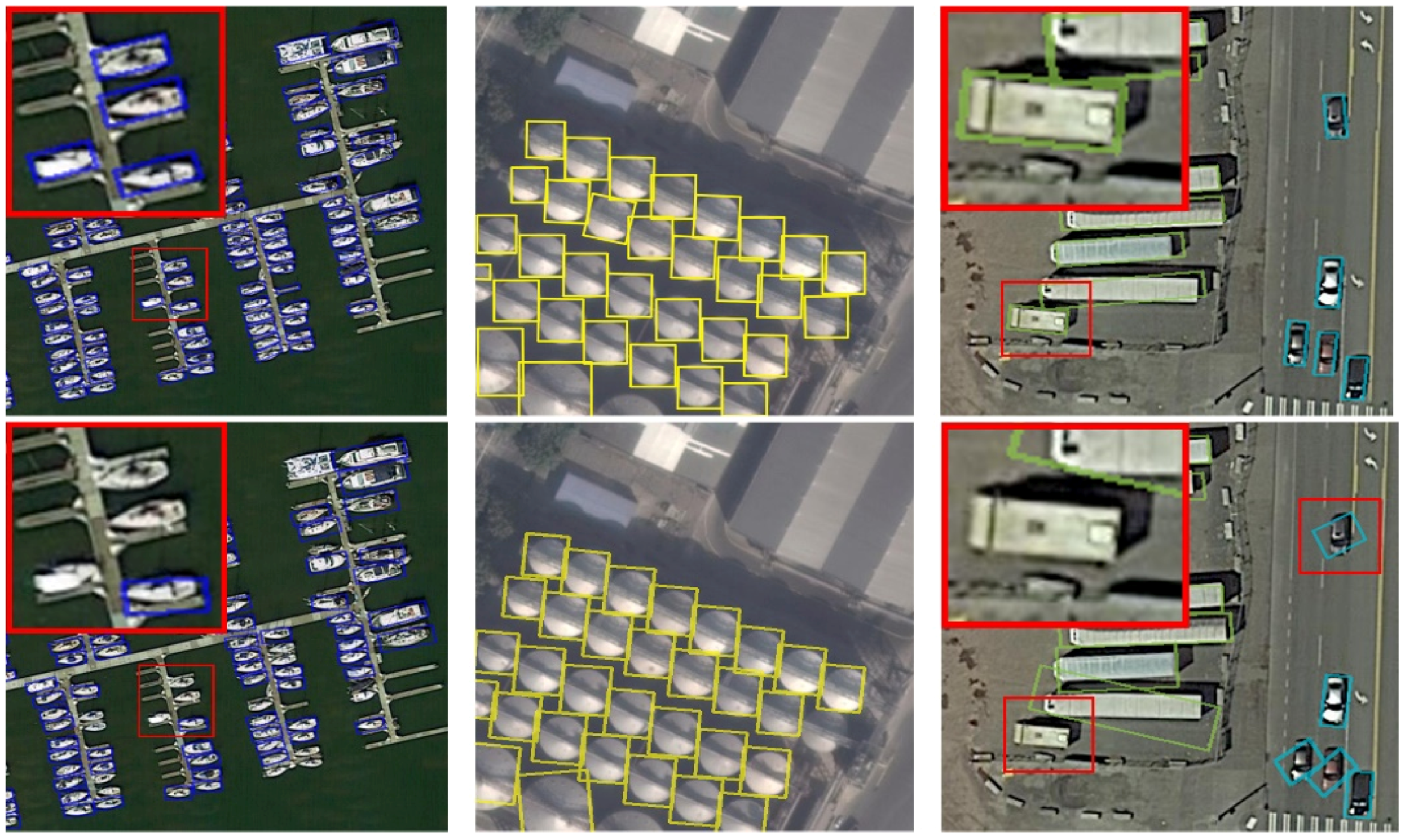
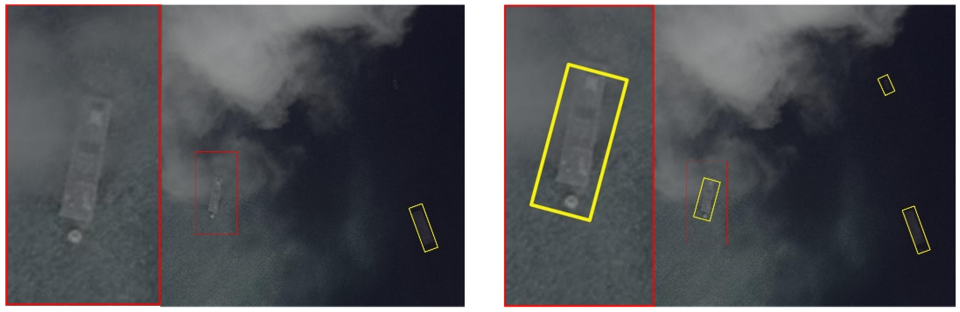
• The multi-feature selection module (MFSM) based on the attention mechanism is designed to reduce the influence of useless features in feature maps in complex backgrounds with a lot of noise.
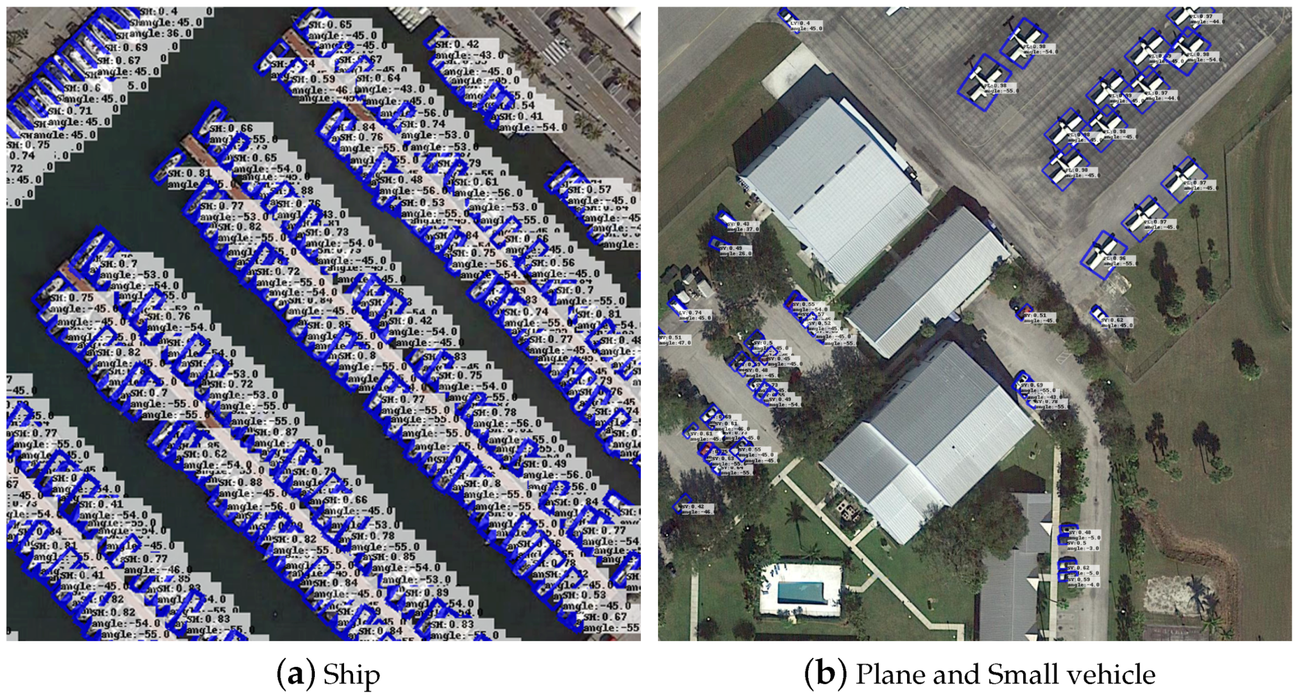
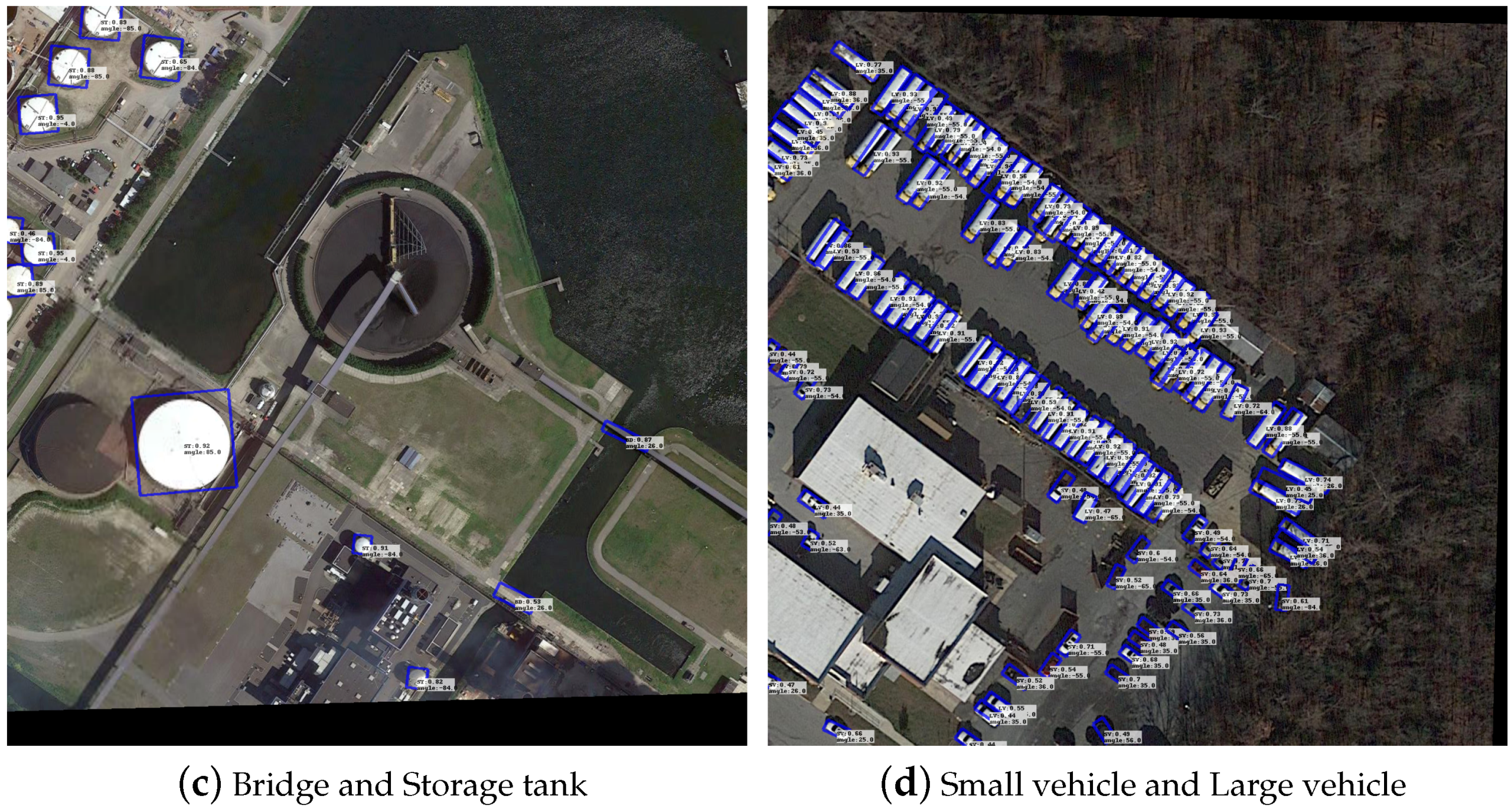
• We propose a novel remote sensing image object detection algorithm that includes a bidirectional multi-scale feature fusion network and a multi-feature selection module. With extensive ablation experiments, we validate the effectiveness of our approach on the standard DOTA dataset and a customized dataset named DOTA-GF. Our proposed method achieves a mAP of 65.1% with the ResNet50 backbone in the DOTA dataset, and 64.1% with the ResNet50 backbone in the DOTA-GF dataset when compared to state-of-the-art methods.

2. Related Work

2.1. Object Detection Algorithms Based on Deep Learning

Object detection algorithms based on deep learning are mainly divided into two categories—one-stage algorithms and two-stage algorithms. The series of algorithms of R-CNN are typical two-stage methods, including R-CNN, Fast R-CNN, and Faster R-CNN [18]. Fast R-CNN proposed RoIpooling and used the convolution network to achieve regression and classification, while Faster R-CNN used the region proposal network (RPN) to replace the selective search and shared feature map with the subsequent classification network. The one-stage methods extract feature maps and predict the categories and locations simultaneously. SSD and YOLO are two typical one-stage methods [19]. The one-stage methods, different from the two-stage methods, are influenced by category imbalances during detection. To tackle such a problem, focal loss [20] is proposed to suppress category imbalance in the one-stage method.

2.2. Arbitrary-Oriented Object Detection

Arbitrary-oriented object detection has been widely used in remote sensing images, aerial images, natural scene texts, etc. These detectors also use rotated bounding boxes to describe the positions of objects, which are more accurate than those using horizontal bounding boxes. Recently, many detectors have been proposed. For example, RRPN [5] uses rotating anchors to improve the qualities of region proposals. R2CNN is a multi-tasking text detector that identifies both rotated and horizontal bounding boxes at the same time. However, object detection in remote sensing images is more difficult, due to multiple categories, multiple scales, and complex backgrounds. Thus, arbitrary-oriented object detection has been proposed in many remote sensing images. R3Det [12] proposed an improved one-stage rotated object detector for accurate object localization by solving the feature misalignment problem. SCRDet [13] proposed an IoU-smooth $L_1$ loss to solve the loss discontinuity caused by the angular periodicity. Reference [21] proposed an anchor-free oriented proposal generator (AOPG) that abandoned the horizontal box-related operations from the network architecture. The AOPG produced coarse-oriented boxes by the coarse location module in an anchor-free manner and refined them into high-quality oriented proposals. Reference [22] proposed an effective oriented object detection method, termed oriented R-CNN. Oriented R-CNN is a general two-stage oriented detector. In the first stage, the oriented region proposal network directly generates high-quality oriented proposals in a nearly cost-free manner. The second stage is the oriented R-CNN head for refining oriented regions of interest and recognizing them.

3. The Proposed Algorithm

We present an overview of our algorithm as sketched in Figure 1. It consists of four parts: The backbone, the bidirectional multi-scale feature fusion network, the multi-feature selection module based on attention mechanism, and the multi-task subnets. We used ResNet50 [23] as our backbone. The bidirectional multi-scale feature fusion network is responsible for fusing high-level semantic information and shallow feature output by the backbone. The multi-feature selection module based on the attention mechanism can select features that are appropriate for classification and regression. After feature selection, the multi-scale feature maps are sent into the classification and regression sub-networks, respectively. Only the center points, widths, and heights of the bounding boxes are predicted by the regression subnet in this case. Through the classification subnet, the categories and angles are predicted.

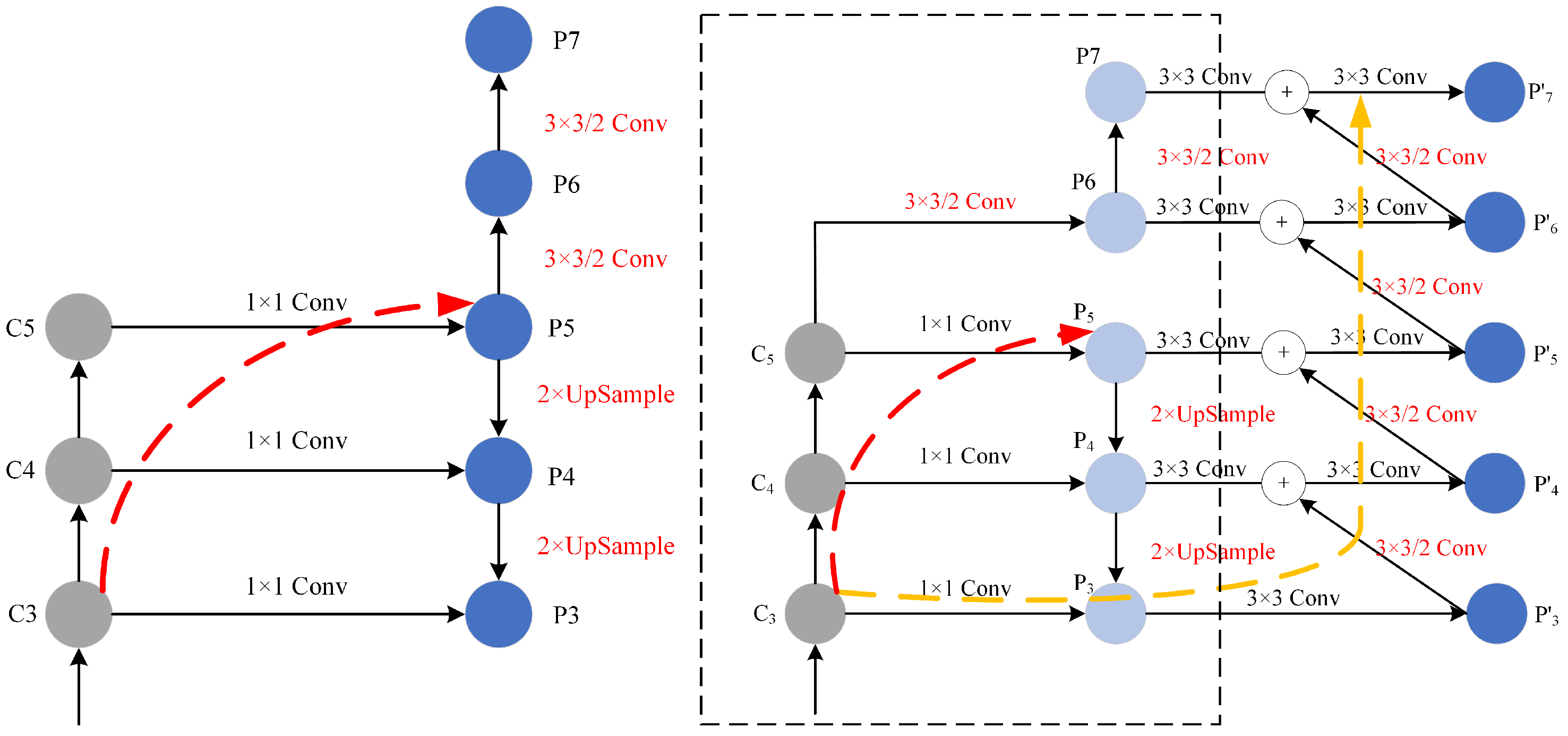
3.1. Bidirectional Multi-Scale Feature Fusion Network

In the early object detection algorithms, such as Faster R-CNN [18], the subsequent classification and regression are usually performed on the feature map of the last layer of the backbone, which is less computationally expensive. However, for the multi-scale object detection, the information of a single-layer feature map is not enough. In 2017, He et al. proposed FPN [20], which fuses high-level features and low-level features, and uses multi-scale fusion feature maps for subsequent detection. RetinaNet [24] also follows the idea of FPN to build a feature pyramid net, as shown in Figure 2a.

Compared with the features extracted only through the last layer of convolution, FPN can use more high-level semantic information and detailed information. The red dotted line in Figure 2a indicates that in FPN, because of the bottom-up path, shallow features need to pass through multilayer networks to reach the top layer, and the information loss is more serious. Taking ResNet50 as an example, the transfer of the $C_3$ layer to the $C_5$ layer needs to go through 27 layers of convolution operations, as shown in Figure 3. The shallow details contained in $P_5$, $P_6$, and $P_7$ are ’lacking’ to be used for subsequent detection. With the addition of the bottom-up fusion path, the detailed texture features of the $C_3$ layer can be transferred to $P_5^{\prime }$, $P_6^{\prime }$, and $P_7^{\prime }$, with only a few layers, as indicated by the yellow dotted line in Figure 2b. Therefore, the loss of shallow features is reduced.

Therefore, we designed a new feature fusion network; a bottom-up path was added to reduce the number of network layers experienced when the shallow features were transferred to the top layer, thereby reducing the loss of shallow features. The detailed information on the network is shown in Figure 2b.

As shown in Figure 2b, $1\times 1Conv$ represents using a $1\times 1$ convolution kernel to perform convolution operations and change the number of channels in the feature map. The $2 \times$ UpSample represents the double upsampling operation of the feature map using bilinear interpolation. The $3\times 3/2Conv$ means using a $3\times 3$ convolution kernel to perform a convolution operation with a stride of 2, reducing the size of the feature map to half of the original size. The output of the backbone is $C_i(i\in 3-5)$, and the feature map after feature fusion is $P_i(i\in 3-7)$. Using $1\times 1$ convolution to reduce the dimension of $C_5$ to obtain $P_5$, $C_5$ is double-downsampled to obtain $P_6$, and $P_6$ is double downsampled to obtain $P_7$. The result of the double-upsampling of $P_5$ is fused with $C_4$ to obtain $P_4$. The result of the double-upsampling of $P_4$ is fused with $C_3$ to obtain $P_3$. $P_i(i\in 3-7)$ combines the information of $C_3$, $C_4$, and $C_5$ at the same time, and contains low-level detailed information and high-level semantic information. Although it has a strong characterization ability for multi-scale objects, the transmission path of shallow features to higher layers is too long, and the feature loss is severe. Therefore, we added a bottom-up path, as shown in the yellow dotted line in Figure 2b. The $3\times 3Conv$ represents a convolution operation with a stride of 1 and a $3\times 3$ convolution kernel. We performed a $3\times 3$ convolution operation on $P_3$ to obtain $P_3^{\prime }$. The result of $P_4^{\prime }$ after the $3\times 3$ convolution and the result of the double-downsampling of $P_3^{\prime }$ were fused to obtain $P_4^{\prime }$. Then $P_5^{\prime }$, $P_6^{\prime }$, and $P_7^{\prime }$ were obtained in the same way.

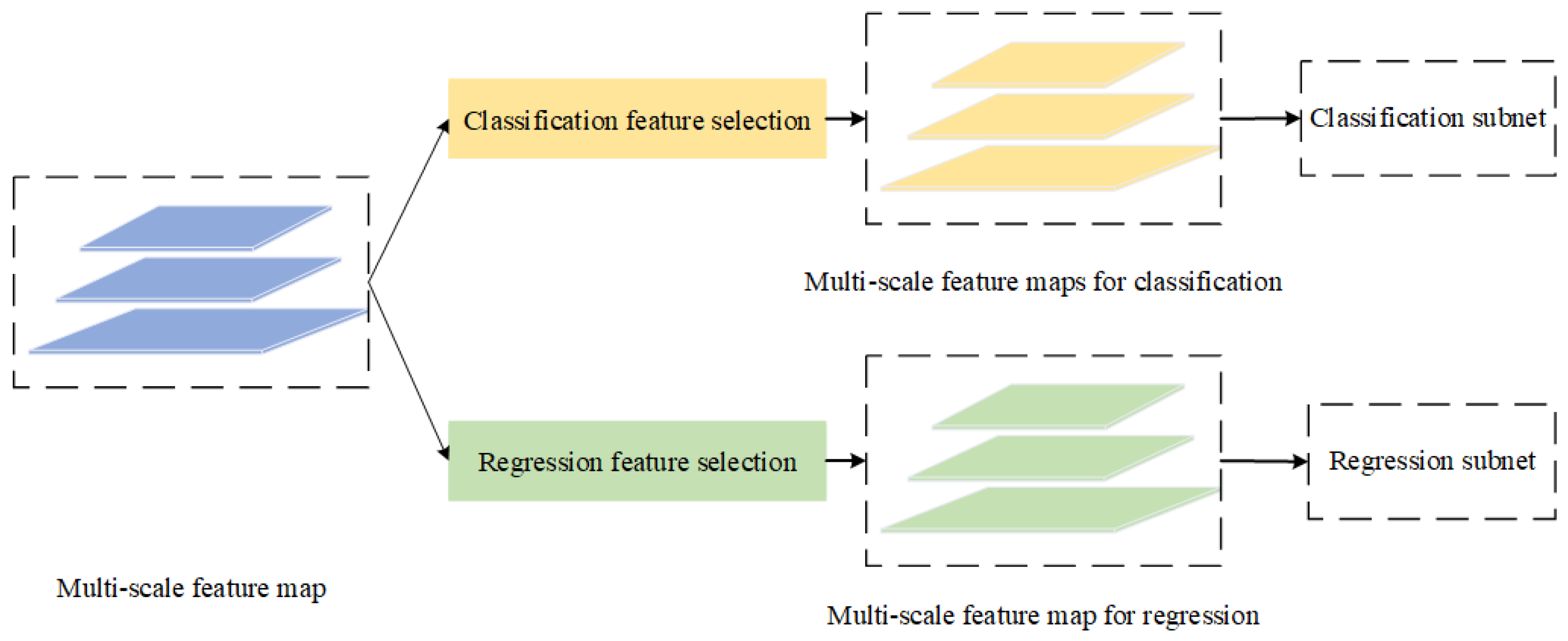
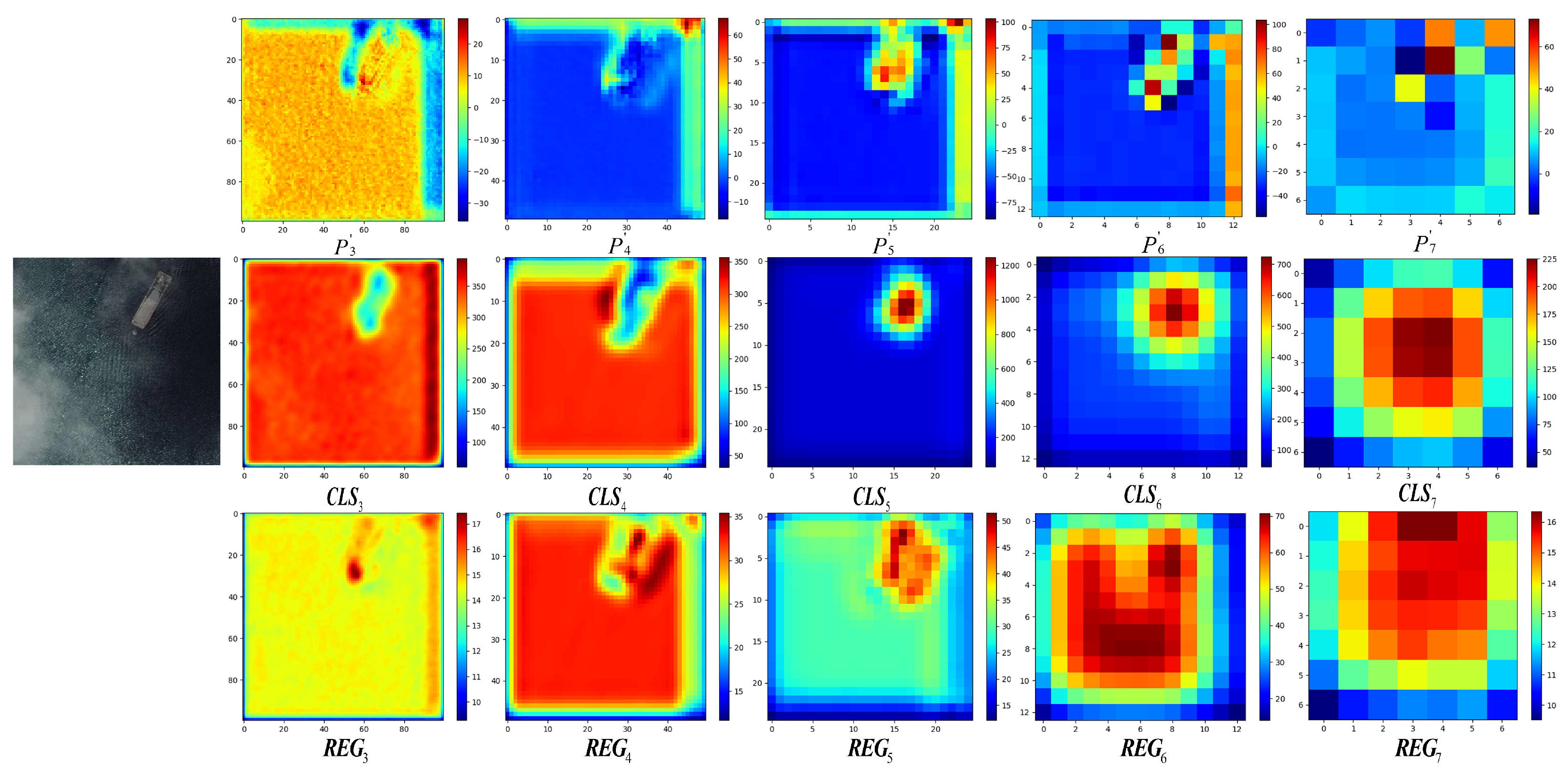
3.2. Multi-Feature Selection Module Based on Attention Mechanism

The complex background of satellite remote sensing images occupies a large area of the whole image. The images taken by domestic satellites, such as GF-2 and GF-6, are not as clear as Google Earth images, which leads to more complex backgrounds of the images, unclear object textures, and sometimes interference from cloud and fog. Directly inputting feature maps of different scales into the subsequent classification and regression sub-networks often fails to obtain ideal results. In recent years, the attention mechanism [25] has achieved great success in computer vision tasks, such as image classification [24] and semantic segmentation [26]. Here, we designed a MFSM. MFSM uses the pixel attention mechanism to select the features suitable for classification and regression, respectively, to reduce the influence of useless information in the feature maps. Different from the spatial attention mechanism, which learns the degree of dependence on different locations in space [27], the pixel attention mechanism learns the degree of dependence on each pixel and adjusts the feature map according to the degree of dependence.

The general one-stage object detection algorithms directly input $P_i^{\prime }(i=3,4,5,6,7)$ into classification subnet and regression subnet. The classification subnet is to predict the category of the bounding box. The regression subnet is primarily responsible for predicting the specific position of the bounding box. The purposes of the two subnets are different. It is inappropriate to use the same feature maps to perform classification and regression tasks at the same time. Therefore, we designed the MFSM. As shown in Figure 4, the multi-scale feature maps are obtained through the feature fusion network, and then are input into two feature selection modules, respectively. Finally, the feature maps after feature selection are input into the classification subnet and regression subnet.

The network details of the feature selection module for classification and the feature selection module for regression are the same, as shown in Figure 5.

The input of the module involves the multi-scale feature map input $P_i^{\prime }(i=3,4,5,6,7)$, output by the feature fusion network and the output of the module is the input series of the feature map $D_i(i=3,4,5,6,7)$ with the same dimensions as the input. The processing process for each input $P_i^{\prime }(i=3,4,5,6,7)$ is shown in Figure 5 and Equations (1) and (2):

$$A_i=\sigma \left[{\varphi }_i\left(P_i^{\prime }\right)\right]$$

(1)

$$D_i=A_i\odot P_i^{\prime }+P_i^{\prime }$$

(2)

where ${\varphi }_i\left(P_i^{\prime }\right)$ means performing four layers of a $3\times 3$ convolution on $P_i^{\prime }$. $\sigma$ is the sigmoid function that converts the value of ${\varphi }_i\left(P_i^{\prime }\right)$ into [0–1] to obtain $A_i$, so that it can converge faster during training. Finally, the result of multiplying the corresponding elements of $P_i^{\prime }$ and $A_i$ is added to $P_i^{\prime }$. The multiplication operation can make the value of the functional information in $P_i^{\prime }$ larger and the value of the useless information smaller. The addition operation refers to the idea of the residual network [23], which can make the network converge faster. This design can make the network adaptively select features suitable for classification or regression.

3.3. Accurate Acquisition of Target Direction Based on Angle Classification

At present, most mainstream algorithms use the idea of regression for angle prediction, and the bounding box is determined by five parameters. The five-parameter regression method has a boundary discontinuity problem [13], which will make the prediction box inaccurate.

Aiming at the loss discontinuity of five-parameter regression, this paper treats the angle prediction as a classification task [28]. The angles are divided into 180 categories. We find that directly dividing the angle into 180 categories will lead to low fault tolerances of adjacent angles. Common methods include the circular smooth label (CSL) [28] method and the densely coded label (DCL) [29] method. Among them, the DCL method is an improvement of the CSL method, which solves the heavy prediction layer and the unfriendly detection of square objects. This paper directly uses the CSL method as the angle classification method. The CSL expression is as follows:

$$S\left(x\right)=\left\{\begin{array}{ccc}\hfill f\left(x\right)& ,\hfill & \hfill if\theta +\tau \le x\le \theta +\tau ,\\ \hfill 0& ,\hfill & \hfill otherwise\end{array}\right.$$

(3)

where $\gamma$ denotes the radius of the window; $\theta$ is the angle of the current ground truth. The circular smooth label is different for each ground truth. $f\left(x\right)$ is the window function, and the Gaussian function is used here, as shown in Equation (4):

$$Gaussian\left(x\right)=a{e}^{\frac{-{(x-b)}^2}{2c^2}}$$

(4)

where a, b, and c are constants $(a>0)$; in this paper, $a=1$, $b=0$, and c is equal to the radius of the window function, which is set to be 6. The CSL [28] can increase the error tolerance to the adjacent angles.

In the paper, the angles of the bounding box are divided into 180 categories. If the angle of the ground truth is $-{90}^{\circ }$, the traditional label of the angle is as follows:

$$label=(1,0,0,0,0,0,0,0\dots 0,0,0,0)$$

(5)

The circular smooth label of the angle is as follows:

$$labe{l}_{csl}=(1,0.86,0.71,0.57,0.43,0.29,0.14,0\dots 0,0,0.14,0.29,0.43,0.57,0.71,0.86)$$

(6)

The detector has two prediction results. In the traditional method, $softmax$ is used to calculate the probabilities of different classes. The corresponding labels are as follows:

$$\left\{\begin{array}{c}\hfill labe{l}_1=(0.03,0.4,0.03,0.03,0.03,0.03,0.03,0.03\dots 0.03,0.03,0.03)\\ \hfill labe{l}_2=(0.03,0.03,0.03,0.03,0.03,0.03,0.4,0.03\dots 0.03,0.03,0.03)\end{array}\right.$$

(7)

In the proposed method, $sigmoid$ is used to calculate the probabilities of different classes. The corresponding labels are as follows:

$$\left\{\begin{array}{c}\hfill labe{l}_1^{*}=(0.1,0.8,0.1,0.1,0.1,0.1,0.1,0.1,0.1\dots 0.1,0.1,0.1,0.1,0.1)\\ \hfill labe{l}_2^{*}=(0.1,0.1,0.1,0.1,0.1,0.1,0.8,0.1,0.1\dots 0.1,0.1,0.1,0.1,0.1)\end{array}\right.$$

(8)

The predicted angle corresponding to $labe{l}_1$ and $labe{l}_1^{*}$ is $-{89}^{\circ }$, and the predicted angle corresponding to $labe{l}_2$ and $labe{l}_2^{*}$ is $-{84}^{\circ }$. Using the cross-entropy loss function as an example. In the traditional method, the losses of $labe{l}_1$ and $labe{l}_2$ to the real label are as follows:

$$\left\{\begin{array}{c}\hfill los{s}_1=-(1\times log\left(0.03\right)+0\times log\left(0.4\right)+0\times log\left(0.03\right)+\dots )=-log\left(0.03\right)\\ \hfill los{s}_2=-(1\times log\left(0.03\right)+\dots +0\times log\left(0.4\right)+0\times log\left(0.03\right)+\dots )=-log\left(0.03\right)\end{array}\right.$$

(9)

It is found that $los{s}_1=los{s}_2$; that is, the $labe{l}_1$ and $labe{l}_2$ have the same loss to the ground truth. However, the predicted angle obtained by $labe{l}_1$ is $-{89}^{\circ }$, which is only $1^{\circ }$ different from the true angle. While the predicted angle obtained by $labe{l}_2$ is $-{84}^{\circ }$, which is $6^{\circ }$ different from the true angle. The first prediction result is obviously more accurate. The analysis shows that directly dividing the angle into 180 categories will lead to low fault tolerance of adjacent angles. In the proposed method, the losses of $labe{l}_1$ and $labe{l}_2$ to the real label are as follows:

$$\left\{\begin{array}{c}\hfill los{s}_1^{*}=-(1\times log\left(0.1\right)+0.86\times log\left(0.8\right)+0.71\times log\left(0.1\right)+\dots )\approx 14.33\\ \hfill los{s}_2^{*}=-(1\times log\left(0.1\right)+0.86\times log\left(0.1\right)+0.71\times log\left(0.8\right)+\dots )\approx 16.12\end{array}\right.$$

(10)

It can be found that $los{s}_1^{*}<los{s}_2^{*}$; that is, the circular smooth label makes the losses of more accurate labels smaller and increases the error tolerance to the adjacent angles.

3.4. Loss Function

The total loss function is as Equation (11):

$$\begin{array}{ccc}\hfill L& =\frac{1}{N}\sum _{n=1}^N{t}_n^{\prime }\sum _{j\in \{x,y,w,h\}}{L}_{reg}(v_{nj}^{\prime },v_{nj})\hfill & \hfill +\frac{{\lambda }_1}{N}\sum _{n=1}^N{L}_{cls}(p_n,t_n)+\frac{{\lambda }_2}{N}\sum _{n=1}^N{L}_{cl{s}_{\theta }}({\theta }_n^{\prime },{\theta }_n)\end{array}$$

(11)

where N indicates the number of anchors, $t_n^{\prime }$ has two values, i.e., 0 and 1, respectively ($t_n^{\prime }=1$ for foreground and $t_n^{\prime }=0$ for background). $v_{ij}^{\prime }$ indicates the predicted offset vector. Moreover, $v_{ij}$ indicates the real offset vector. $t_n$ indicates the label of the object, $p_n$ indicates the probability distribution of various classes calculated by the sigmoid function. Hyperparameters ${\lambda }_1$ and ${\lambda }_2$ are trade-off factors, which control the weights of different loss functions, and their default values are both 1. $L_{reg}$ indicates Smooth $L_1$ Loss [18]. $L_{cls}$ represents the loss of classification in the object category prediction. $L_{cl{s}_{\theta }}$ represents the loss of angle classification in the angle prediction. Both $L_{cls}$ and $L_{cl{s}_{\theta }}$ use focal loss [20].

4. Experimental Results and Discussion

The GPU used in this paper was GTX1660Ti with 6G of memory. The operating system we used was Ubuntu 16.04. The deep learning framework was TensorFlow. ResNet50 was used as the backbone of the network. We conducted experiments on three datasets, and the partitioning criteria were consistent with the references. The DOTA dataset contained a total of 2806 aerial images; 1/2 of the images were selected as the training set, 1/6 as the validation set, and 1/3 as the test set. The HRSC2016 dataset contained 1061 images of ships, of which, training, validation, and testing included 436, 181, and 444 images, respectively. For the self-made DOTA-GF dataset, which contained 2994 images from Google satellites and Chinese satellites, the number of images in training, validation, and test sets were: 1541, 468, and 985.

4.1. Ablation Studies

In this section, we conducted detailed ablation on DOTA to evaluate the effectiveness of each module and illustrate the advance and generalization of the proposed method.

4.1.1. Bidirectional Multi-Scale Feature Fusion Network

To verify the effectiveness of the improved feature fusion network, we used ResNet50 as the backbone and RetinaNet as the embodiment to compare the detection result of the original FPN and the improved feature pyramid network (Improved-FPN) on the DOTA [17] dataset. We mainly considered the average precision (AP) and mean average precision (mAP) of six types of typical objects, including plane (PL), ship (SH), bridge (BG), small vehicle (SV), large vehicle (LV), and storage tank (ST). This is because among the targets in the remote sensing images, the aspect ratio of objects such as plane (PL) and storage tank (ST) was about 1:1, ship (SH), bridge (BG), small vehicle (SV), large vehicle (LV), and other targets were less than 8:1 in length and width. The experimental results are shown in

Table 1. The experimental results of the bidirectional multi-scale feature fusion network.

Method	AP (%)						mAP (%)
	PL	SH	BG	SV	LV	ST
FPN	83.4	62.2	32.3	65.7	48.3	74.9	61.1
our-FPN	$84.5$	$64.6$	$34.0$	$67.2$	$49.2$	$75.5$	$62.5$

.

It can be seen from Table 1 that the Improved-FPN can significantly improve the detection accuracies of typical objects in remote sensing images. Among them, the AP of the ship had the highest increase of 2.4%. That is because many ships in DOTA are small, and the shallow features have a greater impact on the detection results; the bidirectional multi-scale feature fusion network can make full use of the shallow features. The AP of the storage tank has the least increase, which is 0.6%. The mAP of the six types of objects increased by 1.4%. Experimental results show that the improved feature fusion network was more suitable for remote sensing image object detection than the original feature fusion network.

4.1.2. Multi-Feature Selection Module Based on Attention Mechanism

To further prove the effectiveness of the multi-feature selection module, the multi-feature selection module was added to RetinaNet [20] to conduct experiments on DOTA [23]. The comparative experiments of the MFSM with other attention mechanisms were supplemented too. The experimental results with MFSM, SE [30], and CBAM [27] are shown in

Table 2. Experimental results of different attention mechanisms.

Method	AP (%)						mAP (%)
	PL	SH	BG	SV	LV	ST
Baseline	83.4	62.2	32.3	65.7	48.3	74.9	61.1
SE	83.6	64.3	33.4	66.1	$50.1$	74.1	61.9
CBAM	84.4	$64.5$	$33.7$	67.0	49.1	75.2	62.3
MFSM	$84.7$	63.4	33.6	$67.3$	49.5	$76.1$	$62.4$

.

Compared with RetinaNet [20], after adding the multi-feature selection module, the detection accuracies of the six types of typical objects significantly improved with AP increases of 1.2% to 1.6%. The mAP increased by 1.3%. The detection accuracy of the small vehicle had the greatest improvement, and the AP increased by 1.6%. At the same time, MFSM had a better detection performance than SE and CBAM. In SE and CBAM, an attention module was used to process the feature map, and the classification and regression subnets shared the feature map. MFSM processes feature maps for classification and regression, respectively, which can alleviate the conflicts between classification tasks and regression tasks to a certain extent. Therefore, MFSM has a simpler structure, but better performance.

Figure 6 shows a remote sensing image with cloud interference and visualization results of its feature maps. The feature map $P_i^{\prime }(i=3,4,5,6,7)$ was obtained by the feature fusion network. $P_i^{\prime }$ was input into the multi-feature selection network, and the feature map $CL{S}_i(i=3,4,5,6,7)$ for the classification prediction task and the feature map $RE{G}_i(i=3,4,5,6,7)$ for the bounding box prediction task were obtained. In Figure 6, three rows from top to bottom are $P_i^{\prime }$, $CL{S}_i(i=3,4,5,6,7)$, and $RE{G}_i(i=3,4,5,6,7)$. Five columns from left to right are the feature maps of the 3rd, 4th, 5th, 6th, and 7th layers, respectively. For the ship in Figure 6, $P_3^{\prime }$ and $P_4^{\prime }$ in the multi-scale feature maps have greater responses. From $P_3^{\prime }$, $P_4^{\prime }$, $CL{S}_3$, $CL{S}_4$, and $RE{G}_4$, $RE{G}_4$, we can see that after the feature selection, the feature map has a stronger response in the object area. It shows that the multi-feature selection module based on the attention mechanism can select features suitable for classification tasks and regression tasks from multi-scale feature maps and improve the detection accuracy.

4.1.3. Accurate Acquisition of Target Direction Based on Angle Classification

To further prove that turning the angle regression problem into a classification task can improve the remote sensing image detection effect, the angle prediction in RetinaNet is regarded as a classification task with 180 categories, and CSL is used for smoothing. Comparative experiments are performed on the DOTA, and the experimental results are shown in

Table 3. Experimental results of RetinaNet using classification and regression methods to predict angles.

Method	AP (%)						mAP (%)
	PL	SH	BG	SV	LV	ST
Regression	83.4	62.2	32.3	65.7	48.3	74.9	61.1
Classification	$84.2$	$64.9$	$34.5$	$67.6$	$51.5$	$75.8$	$63.1$

. It can be seen from Table 3 that treating the angle prediction as a classification task can significantly improve the detection effect. Among the six types of typical targets, the APs of ships, bridges, small vehicles, and large vehicles increased by 2.7%, 2.2%, 1.9%, and 3.2%, respectively. This is because the aspect ratios of these four types of objects are relatively large, and the use of regression to predict angles has more serious loss discontinuity. For planes and storage tanks with an aspect ratio close to 1, the APs also increased by 0.8% and 0.9%. The experimental results prove that treating the angle prediction as a classification task can effectively improve the detection accuracies of objects with larger aspect ratios.

Figure 7 shows the results of the prediction angle based on the five-parameter regression method. As can be seen from the red boxes in the figure, there is a significant difference between the angles of the detected bounding boxes and the angles of the actual objects, including the large vehicles on the left and the ships on the right.

On the other hand, some visual experiment results based on the proposed classification method are shown in Figure 8. It can be seen that the results obtained by the angle prediction method based on the classification idea are more accurate when detecting the objects, while the angle prediction method based on the classification idea produces more missed detections and false detections

4.2. Results on DOTA

The DOTA [17] dataset contains 15 categories. This paper mainly analyzes six typical objects—ships, planes, bridges, small vehicles, large vehicles, and storage tanks. The evaluation indicators used are AP and mAP. CSL [28], RRPN [5], RetinaNet [20], and Xiao [11] were selected as comparative algorithms. The comparison results of different algorithms are shown in

Table 4. Comparison results of different algorithms on the DOTA dataset.

Category	CSL	RRPN	RetinaNet	Xiao	Proposed
PL	84.2	83.9	83.4	78	$85.7$
SH	64.9	47.2	62.2	65	$66.5$
BG	34.5	32.3	32.3	38	$37.5$
LV	51.5	49.7	48.3	59	54.2
SV	67.6	34.7	65.7	37	$69.2$
ST	75.8	48.8	74.9	50	$77.3$
mAP (%)	63.1	48.0	61.1	55	$65.1$

.

The data in Table 4 show that the mAP of the proposed method is better than most of the mainstream object detection algorithms. The algorithm proposed has achieved the highest AP in four types of objects: planes, ships, small vehicles, and storage tanks. Moreover, the APs of large vehicles and bridges are second only to the highest. The large vehicles in the DOTA dataset are often placed very closely, and adjacent objects have occlusion problems. This is also a problem that we will study in the future. These comparison results show that the algorithm proposed in this paper can effectively detect typical objects in remote sensing images.

The partial visual detection results of the proposed algorithm and the RetinaNet algorithm on the DOTA data set are shown in Figure 9. In order to make the comparison results clearer, some areas are enlarged.

It can be seen from the comparison results in the first column of Figure 9 that when detecting small ships, RetinaNet has a weak ability to characterize small targets, resulting in some missed detections. In the third column of comparative experimental results, RetinaNet also has missed detection when detecting cars. However, the algorithm in this paper obtains better detection results when detecting densely arranged small ships and cars, and the positioning is more accurate. The reason is that the bidirectional multi-scale feature fusion network designed by the algorithm in this paper can improve the representation ability of small targets, the angle information obtained by the idea of classification is also more accurate, and the sensitive feature selection network can further improve the network detection performance.

4.3. Results on DOTA-GF

At present, the remote sensing images in public remote sensing datasets, such as DOTA [17] and NWPU VHR-10 [31], are mainly derived from Google Earth, with only a small amount of data derived from domestic data and lack of military objects. Therefore, we collected 188 GF-2 Satellite images and GF-6 Satellite images with a resolution of $1000\times 1000$ to $4000\times 4000$ and labeled them using the four-point method.

The 138 domestic remote sensing images were added to the training set of DOTA as the DOTA-GF training set. The remaining 50 domestic remote sensing images were added to the DOTA testing set as the DOTA-GF testing set. Then we selected the data containing six types of objects: ships, planes, bridges, small vehicles, large vehicles, and storage tanks, and cropped them to pieces (sizes $600\times 600$) for training. To illustrate the effectiveness of the proposed algorithm, four representative object detection algorithms, CSL [28], RRPN [5], RetinaNet [20], and R3Det [12] were selected for comparison experiments. The detection results of different algorithms are shown in

Table 5. Comparison results of different algorithms on the DOTA-GF dataset.

Category	CSL	RRPN	RetinaNet	R3Det	Proposed
PL	83.6	81.7	83.2	$85.2$	84.6
SH	64.1	46.8	61.0	66.1	$66.3$
BG	35.3	34.8	32.5	35.5	$37.2$
LV	50.4	48.2	50.2	$61.5$	53.8
SV	64.7	33.8	64.5	59.8	$68.6$
ST	72.9	48.6	72.7	70.5	$74.1$
mAP(%)	56.5	49.0	60.7	63.1	$64.1$

.

It can be seen from Table 5 that compared with the four representative algorithms, the algorithm proposed in this paper has achieved the highest AP in four types of objects: ships, bridges, small vehicles, and storage tanks. The APs of planes and large vehicles are also much higher than the highest AP of the four types of algorithms. However, the network structure of R3Det is more complex. Both the training time and the testing time of a single image are longer than the proposed algorithm. Compared with the four comparison algorithms, the mAP of the six typical objects of the proposed algorithm is also the highest. The experimental results show that the algorithm proposed in this paper still has certain advantages on the self-made DOTA-GF dataset.

The detection results of the proposed algorithm and the RetinaNet method on high-resolution images are shown in Figure 10. In order to be more eye-catching, some areas have been partially enlarged.

From the comparison results in Figure 10, it can be seen that when there is cloud interference, RetinaNet cannot accurately capture the characteristics of ships, resulting in missed detection. The algorithm in this chapter has strong anti-cloud and fog interference ability, and can accurately detect ship targets covered by thin clouds.

From the comparison results in Figure 11, it can be seen that when the ship target is relatively small, RetinaNet cannot accurately capture the ship features, resulting in missed detection. Moreover, because of the existence of the proposed FPN module, the algorithm in this paper has a stronger ability to extract small target features and the detection results are more accurate.

From the comparison results in Figure 12, it can be seen that both the algorithm in this paper and RetinaNet have better detection results when detecting objects with large sizes and obvious features, such as aircraft and storage tubes.

4.4. Results of HRSC 2016

HRSC 2016 [32] contains lots of remote sensing ships with a large aspect ratio, scales, and arbitrary orientations. Our method achieves competitive performances on the HRSC2016 dataset. The comparison results are shown in

Table 6. Comparisons with different methods on the HRSC2016 dataset.

Methods	Size	mAP (%)
R2CNN	800 × 800	73.7
RRPN	800 × 800	79.1
RetinaNet	800 × 800	81.7
RoI transformer	512 × 800	86.2
Proposed	800 × 800	$87.1$

.

From Table 6, it can be seen that compared with R2CNN [33], RRPN [5], RetinaNet [20], and the RoI transformer [34], the algorithm in this paper achieves the best detection results, with a mAP of 87.1%. The experimental results verify the effectiveness of the proposed algorithm on the HRSC 2016 dataset.

5. Conclusions

We proposed a new remote sensing image object detection algorithm aimed to target challenges, such as multi-scale objects, complex backgrounds, and boundary problems. In this algorithm, a bidirectional multi-scale feature fusion network was designed to combine the semantic features and shallow detailed features to reduce the loss of information in the process of transferring shallow features to the top layer. A multi-feature selection module based on the attention mechanism was designed to make the network focus on valuable information and select the feature maps appropriate for classification and regression tasks. To avoid the boundary discontinuity problem in the regression process, we treated angle prediction as a classification task rather than a regression task. Finally, experimental results on the DOTA dataset, the DOTA-GF dataset, and the HRSC 2016 dataset show that the proposed algorithm has certain advantages in remote sensing image object detection. However, our proposed method still has limitations in detecting dense objects. In the future, we will ’outlook’ the situation of dense object occlusion and improve our network model to better detect dense objects. The results reported in this paper can be downloaded from https://github.com/xiaojs18/Object-Detection/tree/main/Remote-Detection (accessed on 26 June 2022).

References

- Li, K.; Wan, G.; Cheng, G.; Meng, L.; Han, J. Object detection in optical remote sensing images: A survey and a new benchmark. ISPRS J. Photogramm. Remote Sens. 2020, 159, 296–307. [Google Scholar] [CrossRef]
- Fatima, S.A.; Kumar, A.; Pratap, A.; Raoof, S.S. Object Recognition and Detection in Remote Sensing Images: A Comparative Study. In Proceedings of the 2020 International Conference on Artificial Intelligence and Signal Processing, AISP 2020, Amaravati, India, 10–12 January 2020. [Google Scholar]
- Ma, R.; Chen, C.; Yang, B.; Li, D.; Wang, H.; Cong, Y.; Hu, Z. CG-SSD: Corner guided single stage 3D object detection from LiDAR point cloud. ISPRS J. Photogramm. Remote Sens. 2022, 191, 33–48. [Google Scholar] [CrossRef]
- Hu, Z.; Chen, C.; Yang, B.; Wang, Z.; Ma, R.; Wu, W.; Sun, W. Geometric feature enhanced line segment extraction from large-scale point clouds with hierarchical topological optimization. Int. J. Appl. Earth Obs. Geoinf. 2022, 112, 102858. [Google Scholar] [CrossRef]
- Ma, J.; Shao, W.; Ye, H.; Wang, L.; Wang, H.; Zheng, Y.; Xue, X. Arbitrary-oriented scene text detection via rotation proposals. IEEE Trans. Multimed. 2018, 20, 3111–3122. [Google Scholar] [CrossRef]
- Liu, X.; Meng, G.; Pan, C.A. Scene text detection and recognition with advances in deep learning: A survey. Int. J. Doc. Anal. Recognit. (IJDAR) 2019, 22, 143–162. [Google Scholar] [CrossRef]
- Lin, T.Y.; Dollar, P.; Girshick, R.; He, K.; Hariharan, B.; Belongie, S. Image-to-image translation with conditional adversarial networks. In Proceedings of the 30th IEEE Conference on Computer Vision and Pattern Recognition, Honolulu, HI, USA, 21–26 July 2017; pp. 2117–2125. [Google Scholar]
- Liu, S.; Qi, L.; Qin, H.; Shi, J.; Jia, J. Path Aggregation Network for Instance Segmentation. In Proceedings of the IEEE Computer Society Conference on Computer Vision and Pattern Recognition, Salt Lake City, UT, USA, 18–22 June 2018; pp. 8759–8768. [Google Scholar]
- Guo, C.; Fan, B.; Zhang, Q.; Xiang, S.; Pan, C. AUGFPN: Improving multi-scale feature learning for object detection. In Proceedings of the IEEE Computer Society Conference on Computer Vision and Pattern Recognition, Seattle, WA, USA, 14–19 June 2020; pp. 12592–12601. [Google Scholar]
- Ghiasi, G.; Lin, T.Y.; Le, Q.V. NAS-FPN: Learning scalable feature pyramid architecture for object detection. In Proceedings of the IEEE Computer Society Conference on Computer Vision and Pattern Recognition, Long Beach, CA, USA, 15–20 June 2019; pp. 7029–7038. [Google Scholar]
- Xiao, J.; Zhang, S.; Dai, Y.; Jiang, Z.; Yi, B.; Xu, C. Multiclass Object Detection in UAV Images Based on Rotation Region Network. IEEE J. Miniaturization Air Space Syst. 2020, 1, 188–196. [Google Scholar] [CrossRef]
- Yang, X.; Liu, Q.; Yan, J.; Li, A. R3Det: Refined Single-Stage Detector with Feature Refinement for Rotating Object. In Proceedings of the AAAI Conference on Artificial Intelligence, Online, 2–9 February 2021. [Google Scholar]
- Yang, X.; Yang, J.; Yan, J.; Zhang, Y.; Zhang, T.; Guo, Z.; Sun, X.; Fu, K. SCRDet: Towards More Robust Detection for Small, Cluttered and Rotated Objects. In Proceedings of the 2019 IEEE/CVF International Conference on Computer Vision (ICCV), Seoul, Korea, 27 October–2 November 2019; pp. 8231–8240. [Google Scholar]
- Zhang, Y.; Xiao, J.; Jinye, P.; Ding, Y.; Liu, J.; Guo, Z.; Xiaopeng, Z. Kernel Wiener Filtering Model with Low-Rank Approximation for Image Denoising. Inf. Sci. 2018, 462, 402–416. [Google Scholar] [CrossRef]
- Li, Q.; Mou, L.M.; Jiang, K.; Liu, Q.; Wang, Y.; Zhu, X. Hierarchical Region Based Convolution Neural Network for Multi-scale Object Detection in Remote Sensing Images. In Proceedings of the 2018 IEEE International Geoscience and Remote Sensing Symposium, Valencia, Spain, 22–27 July 2018; pp. 4355–4358. [Google Scholar]
- Xie, H.; Wang, T.; Qiao, M.; Zhang, M.; Shan, G.; Snoussi, H. Robust object detection for tiny and dense targets in VHR aerial images. In Proceedings of the 2017 Chinese Automation Congress, Jinan, China, 20–22 October 2017; pp. 6397–6401. [Google Scholar]
- Xia, G.S.; Bai, X.; Ding, J.; Zhu, Z.; Belongie, S.; Luo, J.; Datcu, M.; Pelillo, M.; Zhang, L. DOTA: A Large-scale Dataset for Object Detection in Aerial Images. In Proceedings of the IEEE Computer Society Conference on Computer Vision and Pattern Recognition, Salt Lake City, UT, USA, 18–22 June 2018; pp. 3974–3983. [Google Scholar]
- Ren, S.; He, K.; Girshick, R.; Sun, J. Faster R-CNN: Towards Real-Time Object Detection with Region Proposal Networks. IEEE Trans. Pattern Anal. Mach. Intell. 2017, 39, 1137–1149. [Google Scholar] [CrossRef] [PubMed]
- Liu, W.; Anguelov, D.; Erhan, D.; Szegedy, C.; Reed, S.; Fu, C.Y.; Berg, A. SSD: Single shot multibox detector. In Proceedings of the 14th European Conference on Computer Vision, Amsterdam, The Netherlands, 11–14 October 2016; pp. 21–37. [Google Scholar]
- Lin, T.Y.; Goyal, P.; Girshick, R.; He, K.; Dollar, P. Focal Loss for Dense Object Detection. IEEE Trans. Pattern Anal. Mach. Intell. 2020, 42, 318–327. [Google Scholar] [CrossRef] [PubMed]
- Cheng, G.; Wang, J.; Li, K.; Xie, X.; Lang, C.; Yao, Y.; Han, J. Anchor-Free Oriented Proposal Generator for Object Detection. IEEE Trans. Geosci. Remote Sens. 2022, 60, 1–11. [Google Scholar] [CrossRef]
- Xie, X.; Cheng, G.; Wang, J.; Yao, X.; Han, J. Oriented R-CNN for Object Detection. In Proceedings of the IEEE/CVF International Conference on Computer Vision (ICCV), Montreal, BC, Canada, 11–17 October 2021; pp. 3520–3529. [Google Scholar]
- He, K.; Zhang, X.; Ren, S.; Sun, J. Deep residual learning for image recognition. In Proceedings of the IEEE Computer Society Conference on Computer Vision and Pattern Recognition, Las Vegas, NV, USA, 27–30 June 2016; pp. 770–778. [Google Scholar]
- Wang, F.; Jiang, M.; Qian, C.; Yang, S.; Li, C.; Zhang, H.; Wang, X.; Tang, X. Residual attention network for image classification. In Proceedings of the 30th IEEE Conference on Computer Vision and Pattern Recognition, Honolulu, HI, USA, 21–26 July 2017; pp. 6450–6458. [Google Scholar]
- Hang, R.; Li, Z.; Liu, Q.; Ghamisi, P.; Bhattacharyya, S.S. Hyperspectral Image Classification With Attention-Aided CNNs. IEEE Trans. Geosci. Remote Sens. 2021, 59, 2281–2293. [Google Scholar] [CrossRef]
- Zhong, Z.; Lin, Z.Q.; Bidart, R.; Hu, X.; Daya, I.B.; Li, Z.; Zheng, W.S.; Li, J.; Wong, A. Squeeze-and-attention networks for semantic segmentation. In Proceedings of the IEEE Computer Society Conference on Computer Vision and Pattern Recognition, Seattle, WA, USA, 14–19 June 2020; pp. 13062–13071. [Google Scholar]
- Woo, S.; Park, J.; Lee, J.Y.; Kweon, I.S. CBAM: Convolutional block attention module. In Proceedings of the Computer Vision—ECCV 2018—15th European Conference, Munich, Germany, 8–14 September 2018; pp. 3–19. [Google Scholar]
- Lin, T.Y.; Goyal, P.; Girshick, R.; He, K.; Dollar, P. Arbitrary-Oriented Object Detection with Circular Smooth Label. Yang Xue Yan Junchi 2020, 12353, 677–694. [Google Scholar]
- Yang, X.; Hou, L.; Zhou, Y.; Wang, W.; Yan, J. Dense Label Encoding for Boundary Discontinuity Free Rotation Detection. In Proceedings of the IEEE Conference on Computer Vision and Pattern Recognition, CVPR 2021, Virtual, 19–25 June 2021; pp. 15819–15829. [Google Scholar]
- Hu, J.; Shen, L.; Sun, G. Squeeze-and-excitation networks. In Proceedings of the IEEE Conference on Computer Vision and Pattern Recognition, Salt Lake City, UT, USA, 18–22 June 2018; pp. 7132–7141. [Google Scholar]
- Cheng, G.; Han, J. A survey on object detection in optical remote sensing images. ISPRS J. Photogramm. Remote Sens. 2016, 117, 11–28. [Google Scholar] [CrossRef]
- Cheng, G.; Han, J.; Zhou, P.; Guo, L. Multi-class geospatial object detection and geographic image classification based on collection of part detectors. ISPRS J. Photogramm. Remote Sens. 2014, 98, 119–132. [Google Scholar] [CrossRef]
- Pang, J.; Li, C.; Shi, J.; Xu, Z.; Feng, H. R2-CNN: Fast Tiny Object Detection in Large-Scale Remote Sensing Images. IEEE Trans. Geosci. Remote Sens. 2019, 57, 5512–5524. [Google Scholar] [CrossRef]
- Ding, J.; Xue, N.; Long, Y.; Xia, G.S.; Lu, Q. Learning roi transformer for oriented object detection in aerial images. In Proceedings of the IEEE/CVF Conference on Computer Vision and Pattern Recognition, Long Beach, CA, USA, 15–20 June 2019; pp. 2849–2858. [Google Scholar]