
Plausible Detection of Feasible Cave Networks Beneath Impact Melt Pits on the Moon Using the Grail Mission


Abstract
:
1. Introduction
2. Data and Methods
2.1. Data
2.2. Method
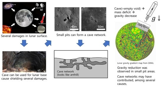
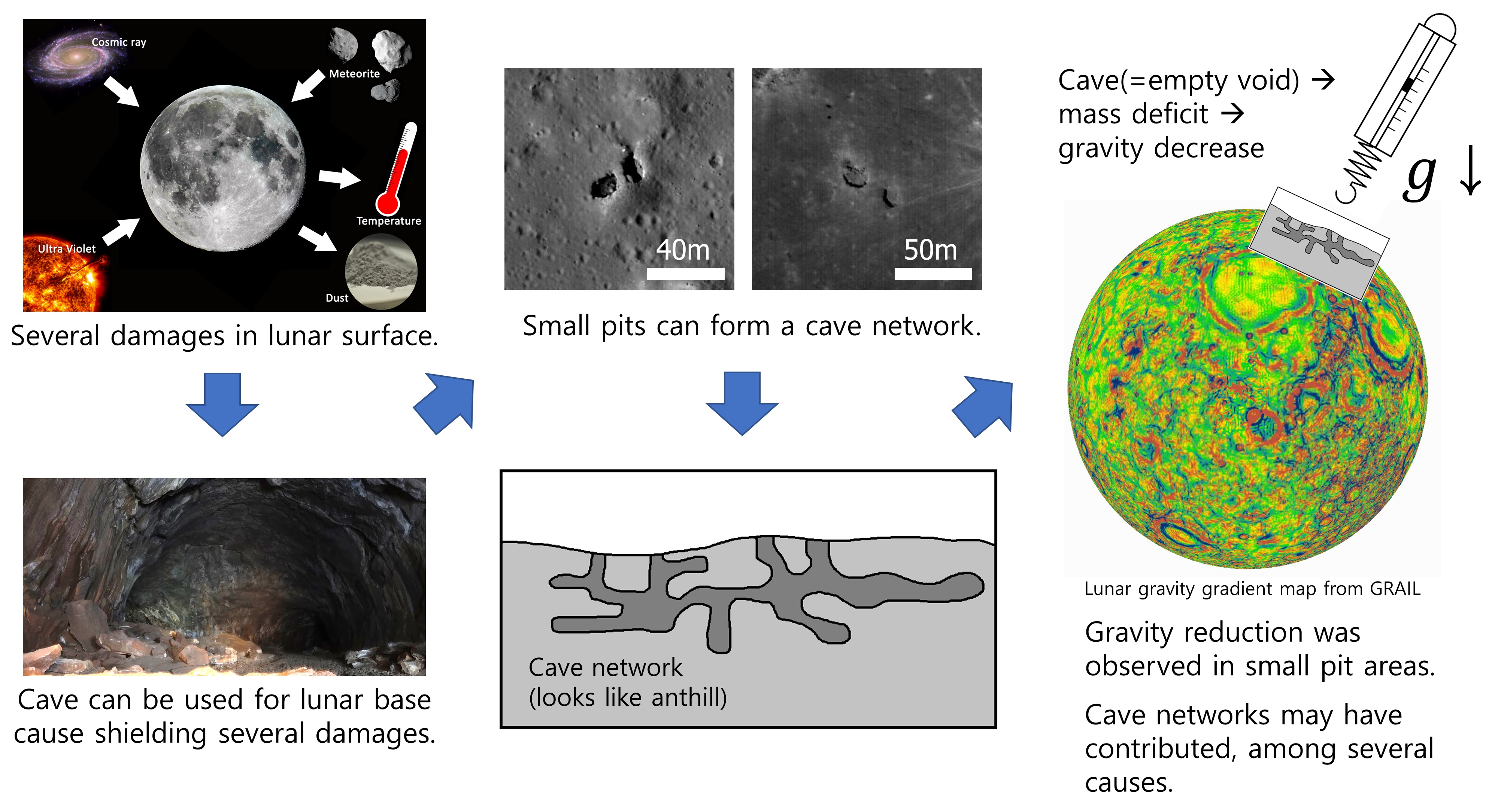
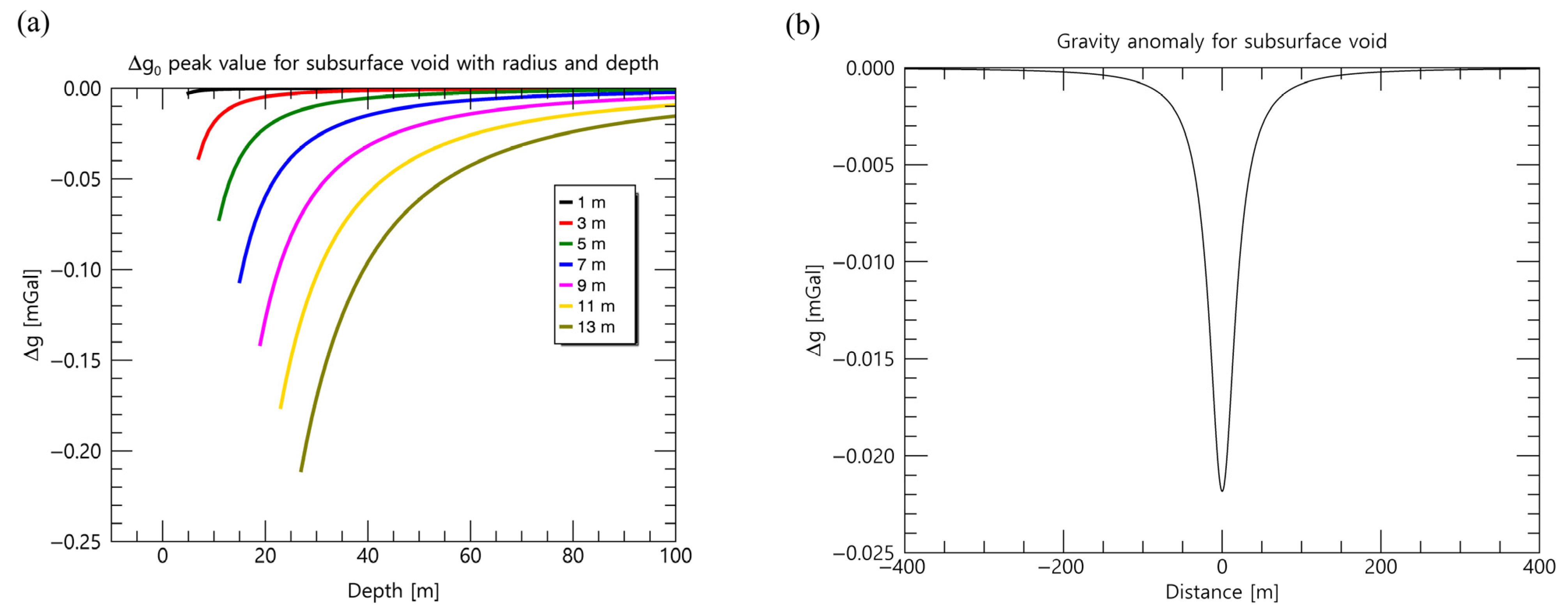
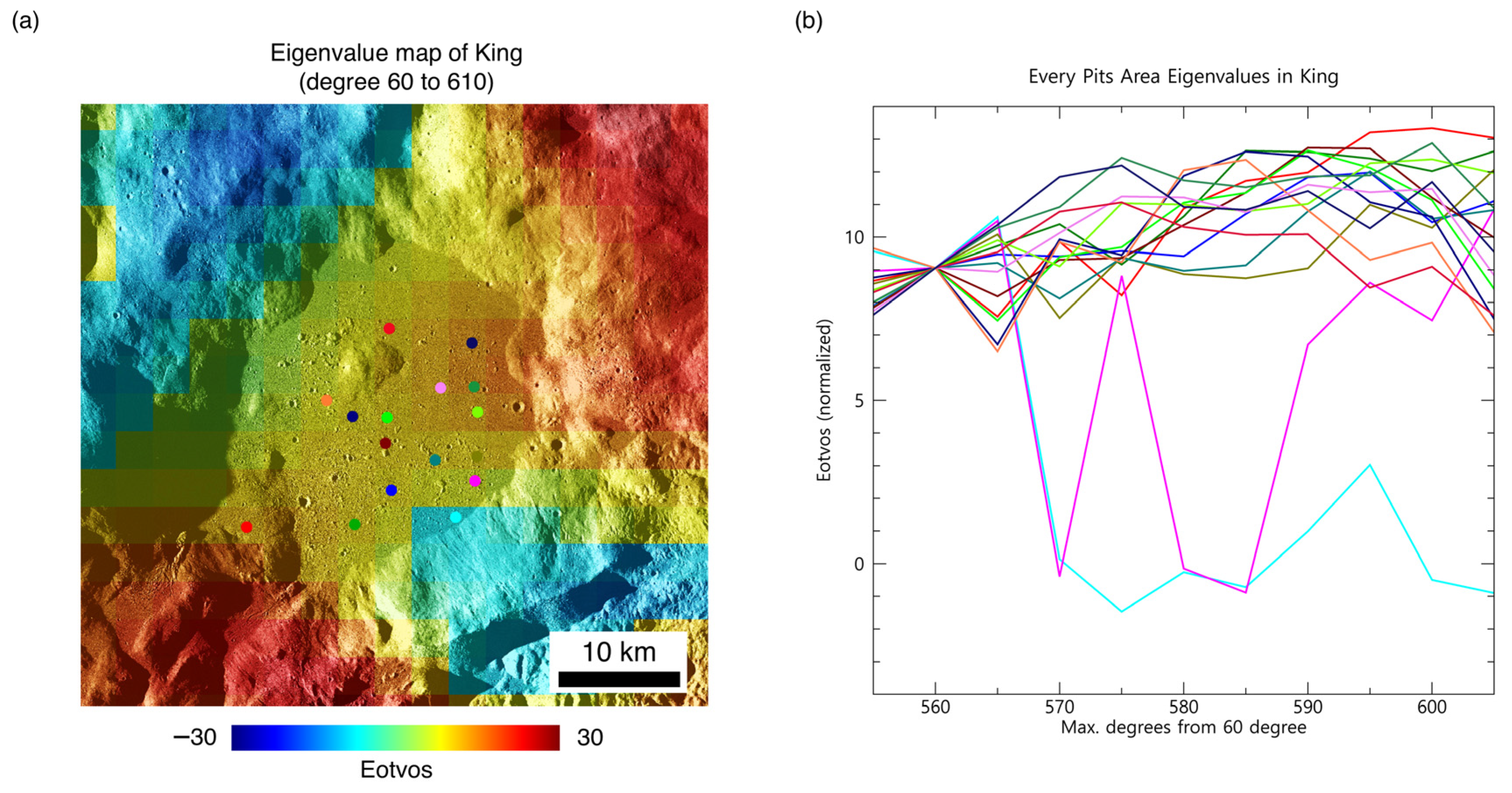
2.2.1. Hypothesis
2.2.2. Research Target
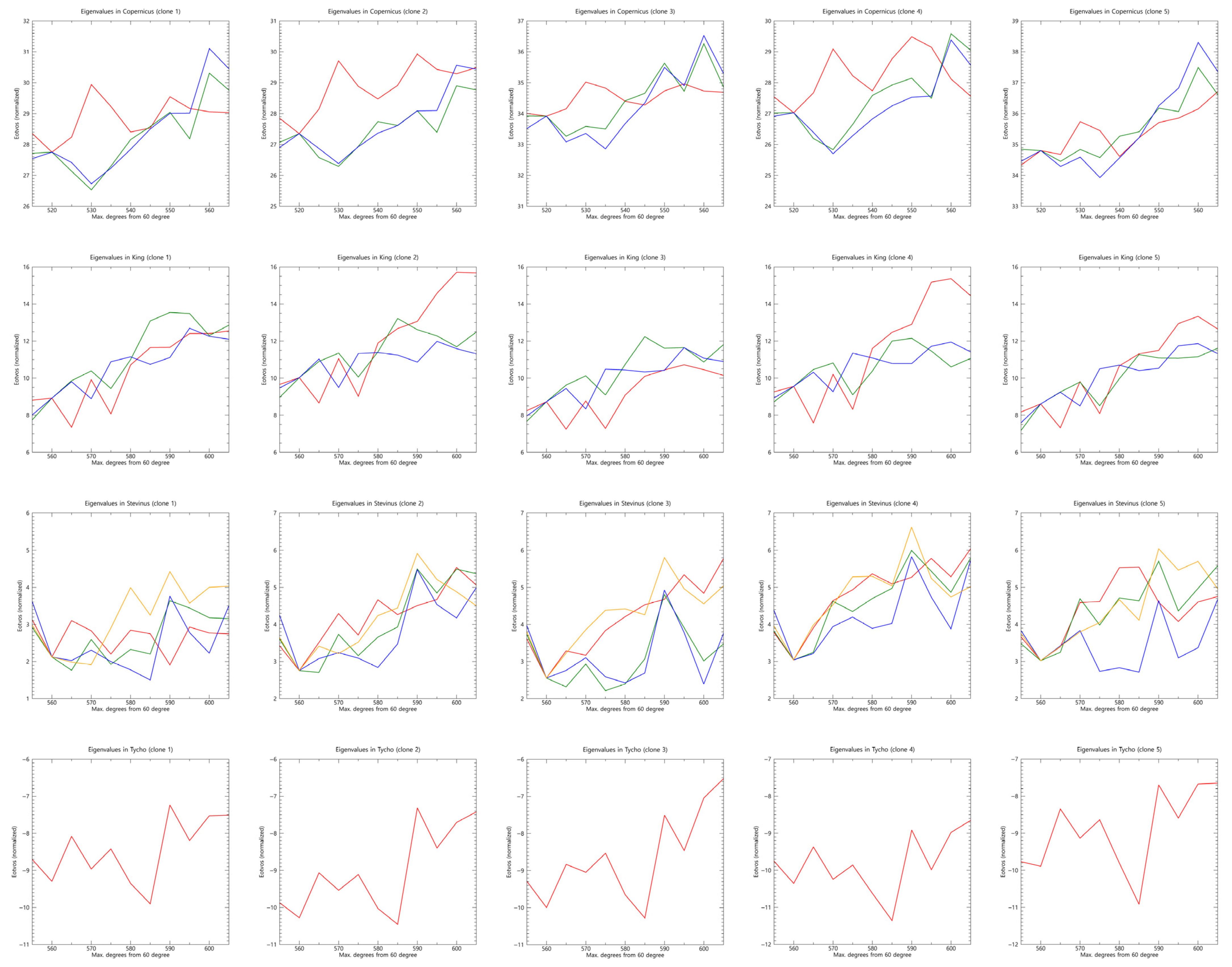
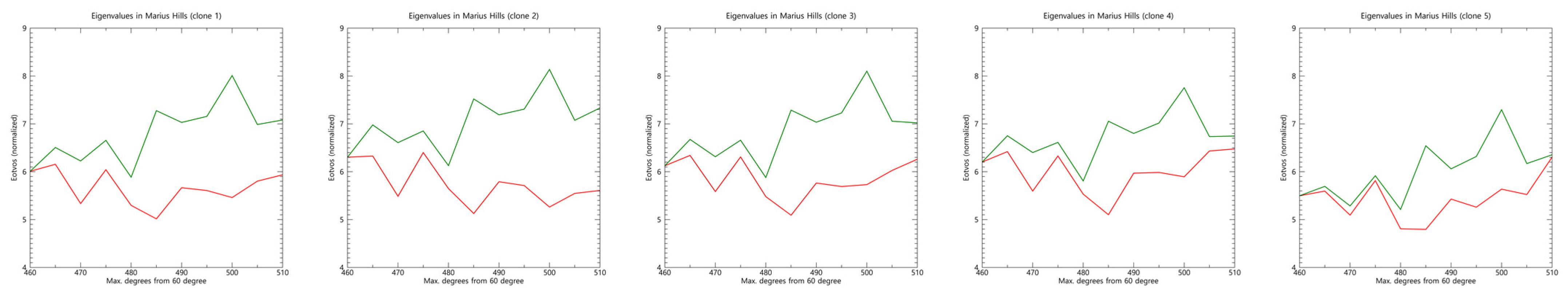
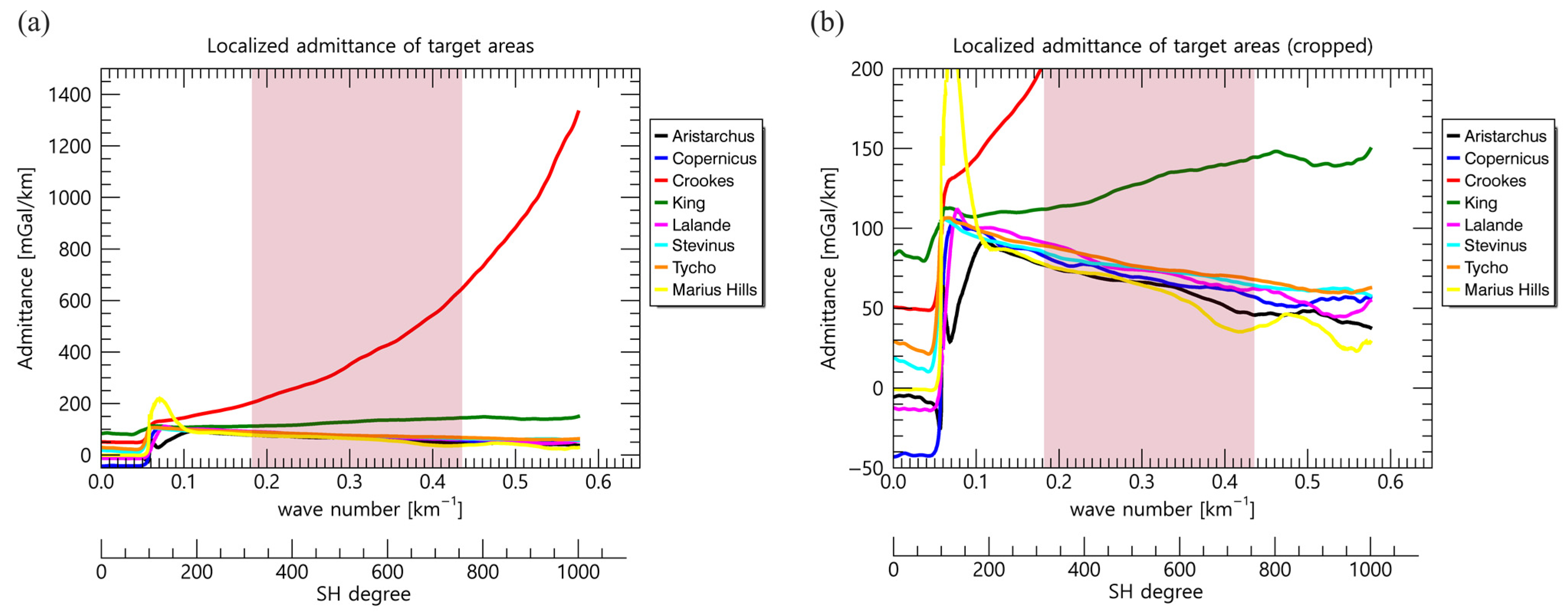
2.2.3. Estimation of Localized Crustal Density
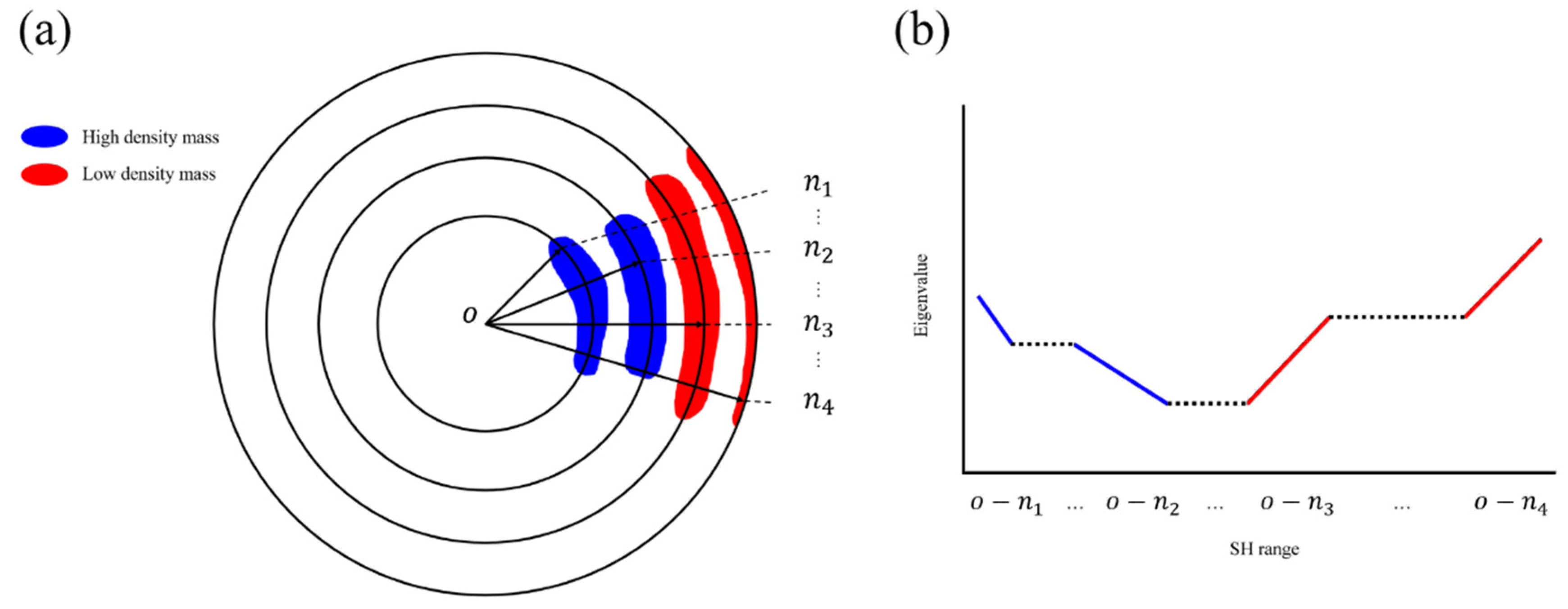
2.2.4. New Processing Method of the Gravity Model
2.2.5. Validation
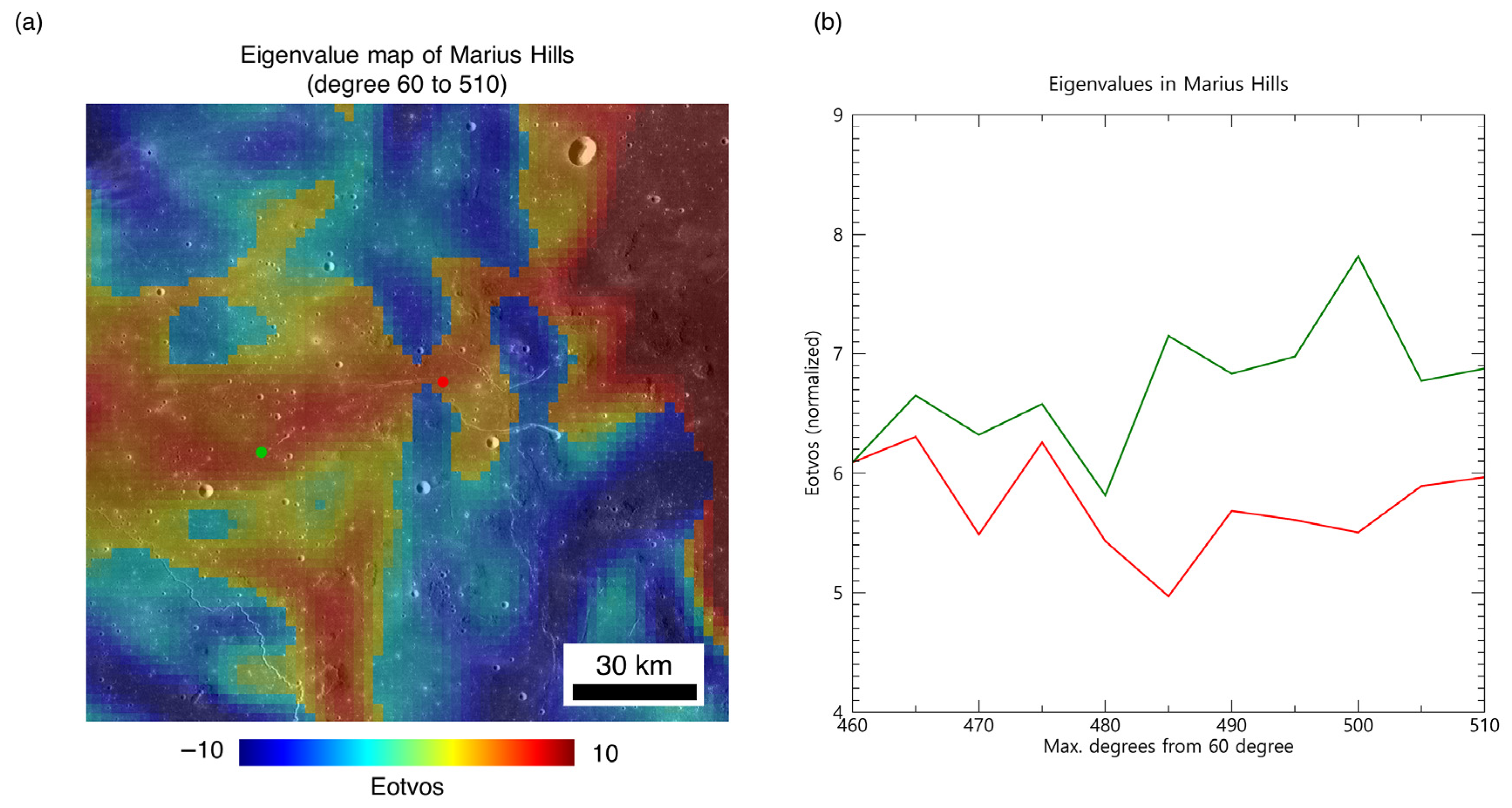
3. Results and Discussion
4. Conclusions
Author Contributions
Funding
Data Availability Statement
Conflicts of Interest
Appendix A

References
- Lauro, S.E.; Pettinelli, E.; Caprarelli, G.; Guallini, L.; Rossi, A.P.; Mattei, E.; Cosciotti, B.; Cicchetti, A.; Soldovieri, F.; Cartacci, M.; et al. Multiple subglacial water bodies below the south pole of Mars unveiled by new MARSIS data. Nat. Astron. 2021, 5, 63–70. [Google Scholar] [CrossRef]
- Pieters, C.M.; Goswami, J.N.; Clark, R.N.; Annadurai, M.; Boardman, J.; Buratti, B.; Combe, J.-P.; Dyar, M.D.; Green, R.; Head, J.W.; et al. Character and Spatial Distribution of OH/H2O on the Surface of the Moon Seen by M3 on Chandrayaan-1. Science 2009, 326, 568–572. [Google Scholar] [CrossRef] [PubMed]
- Cruikshank, D.P.; Wood, C.A. Lunar rilles and Hawaiian volcanic features: Possible analogues. Moon 1972, 3, 412–447. [Google Scholar] [CrossRef]
- Greeley, R. Lava tubes and channels in the lunar Marius Hills. Moon 1971, 3, 289–314. [Google Scholar] [CrossRef]
- Oberbeck, V.R.; Quaide, W.L.; Greeley, R. On the Origin of Lunar Sinuous Rilles. Mod. Geol. 1969, 1, 75–80. [Google Scholar]
- Coombs, C.R.; Hawke, B.R. A Search for Intact Lava Tubes on the Moon: Possible Lunar Base Habitats. In Proceedings of the Second Conference on Lunar Bases and Space Activities of the 21st Century, Houston, TX, USA, 5–8 April 1988; Mendell, W.W., Alred, J.W., Bell, L.S., Cintala, M.J., Crabb, T.M., Durrett, R.H., Finney, B.R., Franklin, H.A., French, J.R., Greenberg, J.S., Eds.; NASA Johnson Space Center: Houston, TX, USA, 1992; p. 219. [Google Scholar]
- Horz, F. Lava tubes—Potential shelters for habitats. In Lunar Bases and Space Activities of the 21st Century; Mendell, W.W., Ed.; Lunar and Planetary Institute: Houston, TX, USA, 1985; pp. 405–412. [Google Scholar]
- Vasavada, A.R.; Bandfield, J.L.; Greenhagen, B.T.; Hayne, P.O.; Siegler, M.A.; Williams, J.P.; Paige, D.A. Lunar equatorial surface temperatures and regolith properties from the Diviner Lunar Radiometer Experiment. J. Geophys. Res. E Planets 2012, 117, E12. [Google Scholar] [CrossRef]
- Kim, E.; Kim, Y.H.; Hong, I.S.; Yu, J.; Lee, E.; Kim, K. Detection of an impact flash candidate on the moon with an educational telescope system. J. Astron. Space Sci. 2015, 32, 121–125. [Google Scholar] [CrossRef]
- Haruyama, J.; Morota, T.; Kobayashi, S.; Sawai, S.; Lucey, P.G.; Shirao, M.; Nishino, M.N. Lunar Holes and Lava Tubes as Resources for Lunar Science and Exploration. In Moon; Springer: Berlin, Heidelberg, 2012; pp. 139–163. ISBN 9783642279690. [Google Scholar]
- Angelis, D.G.; Wilson, J.W.; Clowdsley, M.S.; Nealy, J.E.; Humes, D.H.; Clem, J.M. Lunar lava tube radiation safety analysis. J. Radiat. Res. 2002, 43, S41–S45. [Google Scholar] [CrossRef]
- Cain, J.R. Lunar dust: The Hazard and Astronaut Exposure Risks. Earth Moon Planets 2010, 107, 107–125. [Google Scholar] [CrossRef]
- Stubbs, T.J.; Vondrak, R.R.; Farrell, W.M. A dynamic fountain model for lunar dust. Adv. Space Res. 2006, 37, 59–66. [Google Scholar] [CrossRef]
- Wagner, R.V.; Robinson, M.S. Distribution, formation mechanisms, and significance of lunar pits. Icarus 2014, 237, 52–60. [Google Scholar] [CrossRef]
- Cushing, G.E.; Titus, T.N.; Wynne, J.J.; Christensen, P.R. THEMIS observes possible cave skylights on Mars. Geophys. Res. Lett. 2007, 34, 4–8. [Google Scholar] [CrossRef]
- Cushing, G.E. Candidate cave entrances on Mars. J. Cave Karst Stud. 2012, 74, 33–47. [Google Scholar] [CrossRef]
- Jung, J.; Yi, Y.; Kim, E. Identification of Martian Cave Skylights Using the Temperature Change during Day and Night. J. Astron. Space Sci. 2014, 31, 141–144. [Google Scholar] [CrossRef]
- Haruyama, J.; Hioki, K.; Shirao, M.; Morota, T.; Hiesinger, H.; Van Der Bogert, C.H.; Miyamoto, H.; Iwasaki, A.; Yokota, Y.; Ohtake, M.; et al. Possible lunar lava tube skylight observed by SELENE cameras. Geophys. Res. Lett. 2009, 36, 1–5. [Google Scholar] [CrossRef]
- Haruyama, J.; Hara, S.; Hioki, K.; Morota, T.; Yokota, Y.; Shirao, M.; Hiesinger, H.; van der Bogert, C.H.; Miyamoto, H.; Iwasaki, A.; et al. New Discoveries of Lunar Holes in Mare Tranquillitatis and Mare Ingenii. In Proceedings of the 41st Lunar and Planetary Science Conference, The Woodlands, TX, USA, 1–5 March 2010; p. 1285. [Google Scholar]
- Robinson, M.S.; Ashley, J.W.; Boyd, A.K.; Wagner, R.V.; Speyerer, E.J.; Ray Hawke, B.; Hiesinger, H.; van der Bogert, C.H. Confirmation of sublunarean voids and thin layering in mare deposits. Planet. Space Sci. 2012, 69, 18–27. [Google Scholar] [CrossRef]
- Wagner, R.V.; Robinson, M.S. Occurrence and origin of lunar pits: Observations from a new catalog. In Proceedings of the 52nd Lunar and Planetary Science Conference 2021, Virtual, 15–19 March 2021; p. 2530. [Google Scholar]
- Zuber, M.T.; Smith, D.E.; Lehman, D.H.; Hoffman, T.L.; Asmar, S.W.; Watkins, M.M. Gravity Recovery and Interior Laboratory (GRAIL): Mapping the lunar interior from crust to core. Space Sci. Rev. 2013, 178, 3–24. [Google Scholar] [CrossRef]
- Zuber, M.T.; Smith, D.E.; Watkins, M.M.; Asmar, S.W.; Konopliv, A.S.; Lemoine, F.G.; Melosh, H.J.; Neumann, G.A.; Phillips, R.J.; Solomon, S.C.; et al. Gravity field of the moon from the Gravity Recovery and Interior Laboratory (GRAIL) mission. Science 2013, 339, 668–671. [Google Scholar] [CrossRef]
- Blair, D.M.; Chappaz, L.; Sood, R.; Milbury, C.; Bobet, A.; Melosh, H.J.; Howell, K.C.; Freed, A.M. The structural stability of lunar lava tubes. Icarus 2017, 282, 47–55. [Google Scholar] [CrossRef]
- Theinat, A.K.; Modiriasari, A.; Bobet, A.; Melosh, H.J.; Dyke, S.J.; Ramirez, J.; Maghareh, A.; Gomez, D. Lunar lava tubes: Morphology to structural stability. Icarus 2020, 338, 113442. [Google Scholar] [CrossRef]
- Chappaz, L.; Sood, R.; Melosh, H.J.; Howell, K.C.; Blair, D.M.; Milbury, C.; Zuber, M.T. Evidence of Large Empty Lava Tubes on the Moon using GRAIL Gravity. Geophys. Res. Lett. 2017, 44, 105–112. [Google Scholar] [CrossRef]
- Kaku, T.; Haruyama, J.; Miyake, W.; Kumamoto, A.; Ishiyama, K.; Nishibori, T.; Yamamoto, K.; Crities, S.T.; Michikami, T.; Yokota, Y.; et al. Detection of Lunar Lava Tubes by Lunar Radar Sounder Onboard SELENE (Kaguya). Geophys. Res. Lett. 2017, 48, 1711. [Google Scholar] [CrossRef]
- Kobayashi, T.; Kim, J.-H.; Lee, S.R.; Song, K.-Y. Nadir Detection of Lunar Lava Tube by Kaguya Lunar Radar Sounder. IEEE Trans. Geosci. Remote Sens. 2021, 59, 7395–7418. [Google Scholar] [CrossRef]
- Goossens, S.; Lemoine, F.G.; Sabaka, T.J.; Nicholas, J.B.; Mazarico, E.; Rowlands, D.D.; Loomis, B.D.; Chinn, D.S.; Neumann, G.A.; Smith, D.E.; et al. A Global Degree and Order 1200 Model of the Lunar Gravity Field Using GRAIL Mission Data. In Proceedings of the 47th Annual Lunar and Planetary Science Conference, The Woodlands, TX, USA, 21–25 March 2016; p. 1484. [Google Scholar]
- Konopliv, A.S.; Park, R.S.; Yuan, D.N.; Asmar, S.W.; Watkins, M.M.; Williams, J.G.; Fahnestock, E.; Kruizinga, G.; Paik, M.; Strekalov, D.; et al. The JPL lunar gravity field to spherical harmonic degree 660 from the GRAIL Primary Mission. J. Geophys. Res. E Planets 2013, 118, 1415–1434. [Google Scholar] [CrossRef]
- Konopliv, A.S.; Park, R.S.; Yuan, D.-N.; Asmar, S.W.; Watkins, M.M.; Williams, J.G.; Fahnestock, E.; Kruizinga, G.; Paik, M.; Strekalov, D.; et al. High-resolution lunar gravity fields from the GRAIL Primary and Extended Missions. Geophys. Res. Lett. 2014, 41, 1452–1458. [Google Scholar] [CrossRef]
- Lemoine, F.G.; Goossens, S.; Sabaka, T.J.; Nicholas, J.B.; Mazarico, E.; Rowlands, D.D.; Loomis, B.D.; Chinn, D.S.; Caprette, D.S.; Neumann, G.A.; et al. High-degree gravity models from GRAIL primary mission data. J. Geophys. Res. E Planets 2013, 118, 1676–1698. [Google Scholar] [CrossRef]
- Lemoine, F.G.; Goossens, S.; Sabaka, T.J.; Nicholas, J.B.; Mazarico, E.; Rowlands, D.D.; Loomis, B.D.; Chinn, D.S.; Neumann, G.A.; Smith, D.E.; et al. GRGM900C: A degree 900 lunar gravity model from GRAIL primary and extended mission data. Geophys. Res. Lett. 2014, 41, 3382–3389. [Google Scholar] [CrossRef]
- Park, R.S.; Konopliv, A.S.; Yuan, D.N.; Asmar, S.; Watkins, M.M.; Williams, J.; Smith, D.E.; Zuber, M.T. A high-resolution spherical harmonic degree 1500 lunar gravity field from the GRAIL mission. In Proceedings of the AGU Fall Meeting, San Francisco, CA, USA, 14–18 December 2015; Volume 2015, p. G41B-01. [Google Scholar]
- Zuber, M.T.; Smith, D.E.; Goossens, S.J.; Neumann, G.A.; Lemoine, F.G.; Mazarico, E.; Genova, A.; Rowland, D.D. Exploring the Depth Distribution of Lunar Crustal Mass Anomalies Using GRAIL Gravity and LOLA Topography. In Proceedings of the 47th Lunar and Planetary Science Conference, The Woodlands, TX, USA, 21–25 March 2016; p. 2105. [Google Scholar]
- Goossens, S.; Sabaka, T.J.; Wieczorek, M.A.; Neumann, G.A.; Mazarico, E.; Lemoine, F.G.; Nicholas, J.B.; Smith, D.E.; Zuber, M.T. High-Resolution Gravity Field Models from GRAIL Data and Implications for Models of the Density Structure of the Moon′s Crust. J. Geophys. Res. Planets 2020, 125, 1–31. [Google Scholar] [CrossRef]
- Lowrie, W. Fundamentals of Geophysics; Cambridge University Press: Cambridge, UK, 2007; ISBN 9780511807107. [Google Scholar]
- Hong, I.S.; Yi, Y.; Kim, E. Lunar pit craters presumed to be the entrances of Lava caves by analogy to the Earth lava tube pits. J. Astron. Space Sci. 2014, 31, 131–140. [Google Scholar] [CrossRef]
- Okubo, C.H.; Martel, S.J. Pit crater formation on Kilauea volcano, Hawaii. J. Volcanol. Geotherm. Res. 1998, 86, 1–18. [Google Scholar] [CrossRef]
- Wieczorek, M.A.; Meschede, M. SHTools: Tools for Working with Spherical Harmonics. Geochem. Geophys. Geosyst. 2018, 19, 2574–2592. [Google Scholar] [CrossRef]
- Andrews-Hanna, J.C.; Asmar, S.W.; Head, J.W.; Kiefer, W.S.; Konopliv, A.S.; Lemoine, F.G.; Matsuyama, I.; Mazarico, E.; McGovern, P.J.; Melosh, H.J.; et al. Ancient Igneous Intrusions and Early Expansion of the Moon Revealed by GRAIL Gravity Gradiometry. Science 2013, 339, 675–678. [Google Scholar] [CrossRef] [PubMed]
- Wieczorek, M.A.; Neumann, G.A.; Nimmo, F.; Kiefer, W.S.; Taylor, G.J.; Melosh, H.J.; Phillips, R.J.; Solomon, S.C.; Andrews-Hanna, J.C.; Asmar, S.W.; et al. The crust of the moon as seen by GRAIL. Science 2013, 339, 671–675. [Google Scholar] [CrossRef] [PubMed]
- Watts, A.B. Isostasy and Flexure of the Lithosphere; Cambridge University Press: Cambridge, UK, 2001; ISBN 9780521006002. [Google Scholar]
- Simons, F.J.; Dahlen, F.A.; Wieczorek, M.A. Spatiospectral concentration on a sphere. SIAM Rev. 2006, 48, 504–536. [Google Scholar] [CrossRef]
- Wieczorek, M.A.; Simons, F.J. Localized spectral analysis on the sphere. Geophys. J. Int. 2005, 162, 655–675. [Google Scholar] [CrossRef]
- Wieczorek, M.A.; Simons, F.J. Minimum-variance multitaper spectral estimation on the sphere. J. Fourier Anal. Appl. 2007, 13, 665–692. [Google Scholar] [CrossRef]
- Wieczorek, M.A. Gravity and Topography of the Terrestrial Planets. In Treatise on Geophysics, 2nd ed.; Elsevier: Amsterdam, The Netherlands, 2015; Volume 10, ISBN 9780444538031. [Google Scholar]
- Pedersen, L.B.; Rasmussen, T.M. The gradient tensor of potential field anomalies: Some implications on data collection and data processing of maps. Geophysics 1990, 55, 1558–1566. [Google Scholar] [CrossRef]
- Deutsch, A.N.; Neumann, G.A.; Head, J.W.; Wilson, L. GRAIL-identified gravity anomalies in Oceanus Procellarum: Insight into subsurface impact and magmatic structures on the Moon. Icarus 2019, 331, 192–208. [Google Scholar] [CrossRef]
- Evans, A.J.; Soderblom, J.M.; Andrews-Hanna, J.C.; Solomon, S.C.; Zuber, M.T. Identification of buried lunar impact craters from GRAIL data and implications for the nearside maria. Geophys. Res. Lett. 2016, 43, 2445–2455. [Google Scholar] [CrossRef]
- Sood, R.; Chappaz, L.; Melosh, H.J.; Howell, K.C.; Milbury, C.; Blair, D.M.; Zuber, M.T. Detection and characterization of buried lunar craters with GRAIL data. Icarus 2017, 289, 157–172. [Google Scholar] [CrossRef]
- Isaacson, P.J.; Pieters, C.M.; Besse, S.; Clark, R.N.; Head, J.W.; Klima, R.L.; Mustard, J.F.; Petro, N.E.; Staid, M.I.; Sunshine, J.M.; et al. Remote compositional analysis of lunar olivine-rich lithologies with Moon Mineralogy Mapper (M3) spectra. J. Geophys. Res. E Planets 2011, 116, 1–17. [Google Scholar] [CrossRef]
- Ashley, J.W.; Robinson, M.S.; Hawke, B.R.; Van Der Bogert, C.H.; Hiesinger, H.; Sato, H.; Speyerer, E.J.; Enns, A.C.; Wagner, R.V.; Young, K.E.; et al. Geology of the King crater region: New insights into impact melt dynamics on the Moon. J. Geophys. Res. E Planets 2012, 117, 1–13. [Google Scholar] [CrossRef]


| Name | Latitude | Longitude | No. Pits > 5 m Wide |
|---|---|---|---|
| King | 6.5°N | 119.8°E | 51 (62) |
| Tycho | 43.3°S | 11.2°W | 31 (24) |
| Copernicus | 9.6°N | 20.1°W | 17 (32) |
| Lalande | 4.4°S | 8.6°W | 19 (8) |
| Stevinus | 32.5°S | 54.1°E | 16 (26) |
| Aristarchus | 23.7°N | 47.5°W | 13 (14) |
| Crookes | 10.4°S | 165.1°W | 11 (14) |
| Name | Crustal Density [kg/m3] | Depth [km] |
|---|---|---|
| King | 2147.61 | −0.94 |
| Tycho | 2659.97 | 1.00 |
| Copernicus | 2618.09 | 1.23 |
| Lalande | 2933.59 | 1.35 |
| Stevinus | 2432.88 | 0.82 |
| Aristarchus | 2369.62 | 1.10 |
| Crookes | 2107.24 | −3.63 |
| Name | Max. Degree and Order |
|---|---|
| King | 606 |
| Tycho | 609 |
| Copernicus | 564 |
| Lalande | 567 |
| Stevinus | 603 |
| Aristarchus | 534 |
| Crookes | 612 |
Publisher’s Note: MDPI stays neutral with regard to jurisdictional claims in published maps and institutional affiliations. |
© 2022 by the authors. Licensee MDPI, Basel, Switzerland. This article is an open access article distributed under the terms and conditions of the Creative Commons Attribution (CC BY) license (https://creativecommons.org/licenses/by/4.0/).
Share and Cite
Hong, I.-S.; Yi, Y. Plausible Detection of Feasible Cave Networks Beneath Impact Melt Pits on the Moon Using the Grail Mission. Remote Sens. 2022, 14, 3926. https://doi.org/10.3390/rs14163926
Hong I-S, Yi Y. Plausible Detection of Feasible Cave Networks Beneath Impact Melt Pits on the Moon Using the Grail Mission. Remote Sensing. 2022; 14(16):3926. https://doi.org/10.3390/rs14163926
Chicago/Turabian StyleHong, Ik-Seon, and Yu Yi. 2022. "Plausible Detection of Feasible Cave Networks Beneath Impact Melt Pits on the Moon Using the Grail Mission" Remote Sensing 14, no. 16: 3926. https://doi.org/10.3390/rs14163926
APA StyleHong, I.-S., & Yi, Y. (2022). Plausible Detection of Feasible Cave Networks Beneath Impact Melt Pits on the Moon Using the Grail Mission. Remote Sensing, 14(16), 3926. https://doi.org/10.3390/rs14163926