Abstract
In this work, the parameter identifiability of sensor position perturbations in a distributed network is analyzed through establishing the link between rank of the Jacobian matrix and parameter identifiability under Gaussian noise. Here, the calibration is classified as either external or internal, dependent on whether auxiliary sources are exploited. It states that, in the case of internal calibration, sensor position perturbations can be precisely calibrated when the position of a sensor and orientation to a second sensor along with the coordinate of a third sensor along some axis, are known. In the case of external calibration where auxiliary sources are introduced to support the process, the identifiability condition for configuration calibration is to have at least three noncollinear auxiliary sources with the distributed sensor network avoiding the collinear and coplanar geometries. As the assumption of small perturbations is considered, the parameter identifiability is capable of being measured by virtue of the Bayesian Cramer–Rao lower bound (BCRLB), after asymptotical tightness of the BCRLB is verified. Simulations corroborate well with the theoretical development.
1. Introduction
In the problem of source localization, time delays (TDs) between spatially distributed sensors and the source are processed jointly to locate the source in a network. It is resultantly obvious that any phenomenon which introduces uncertainty into the relation between TDs and the source position would tend to degrade source localization precision. In practical terms, such a situation occurs when sensor locations are not known with great precision, e.g., with a network deployed from the air or a flexible towed network. In [1], it was concluded that sensor position uncertainties could make substantial contributions to the overall source localization error. In [2,3], the increase in the mean square error (MSE) of source localization due to sensor position uncertainties was derived. They both remark that, aside from the sensor geometry and signal-to-noise ratio (SNR), source localization accuracy is highly vulnerable to sensor position uncertainties. As a result, configuration calibration appears crucial, which attempts to refine sensor positions before the sensor network is put into use.
An earlier series of papers realized the problem of uncertainty in array shape [4,5,6,7,8,9,10,11,12,13,14]. It is straightforward to equip each sensor with a global positioning system (GPS) to obtain its position information, but this adds to the expense and power requirement of the sensor and increases its susceptibility to detection [4]. Signal coherence and accurate source localization demand a centimeter-level sensor positioning accuracy which cannot be provided by the GPS, for the GPS only achieves a meter-level positioning accuracy with the current state of art [5]. In [6], it is reported that if all sensor positions are unknown, inter-sensor measurements only produce relative sensor positions with translation and rotation uncertainties. In [7,8], it is stated that the use of auxiliary sources at known locations into source localization can reduce the TD estimation error due to sensor position perturbations. In two classic papers [9,10], Rockah and Schultheiss analyzed parameter identifiability of the problem of joint nonlinear array shape calibration and source bearings estimation through using the hybrid Cramer–Rao lower bound (CRLB) for the first time. It declares that accurate array shape calibration can be completed when the precise knowledge of the location of a sensor and orientation to a second sensor is required with at least three noncollinear sources. In [11,12], it is indicated that a nominally linear sensor array enables self-calibrating with at least two noncollinear sources if the hybrid CRLB is tight and the identifiability condition in [9] is insured. In [13,14], the parameter identifiability for joint estimation of target parameters and system deviations in a multiple-input multiple-output (MIMO) system was investigated by judging positive definiteness of the Fisher information matrix (FIM). In [15,16,17,18], the parameter identifiability of TD-based elliptic localization in MIMO systems was studied by comparing the number of measurement equations and that of unknowns. The optimal sensor placement, under the presence of sensor position perturbations, was designed by maximizing the determinant of the underlying FIM in [19,20,21]. Sensor position perturbations change TDs nonlinearly and, further, changes of TDs are equivalent to phase shifts varying with frequency. Therefore, the similarities of TDs and phase shifts are obvious. The impact of phase perturbations at ends of the transmitter and receiver on source localization accuracy was discussed in [22]. The identifiability of phase perturbations in MIMO systems was analyzed in [23].
For the problem studied herein, all the unknown sensor position perturbations, are random with available prior distribution. Based on the central limited theorem (CLT) [24] and the error model in [25,26], it is reasonable to assume that sensor position perturbations obey a zero-mean Gaussian distribution. So, the Bayesian CRLB (BCRLB) bounds the MSE of any estimator for the random unknowns [27] and also serves as a useful tool for the identifiability issue. Moreover, if the BCRLB reaches zero at sufficiently high SNRs and is tight [28,29], which means that parameter estimation can be made as accurate as desired, and these random parameters are identifiable. Conversely, if the BCRLB converges to a constant error covariance at sufficiently high SNRs, which translates to that all the unknowns, cannot be estimated without error, these random parameters are unidentifiable [11]. It is because some limitations cannot be fulfilled, such as the required minimal amount of auxiliary sources and non-pathological geometries, which are sometimes called as observability condition [30,31]. Unfortunately, most of the above papers concerning parameter identifiability confine their attention to the two-dimensional (2-D) framework and do not consider the complicated three-dimensional (3-D) case. They only consider the information between sensors and sources for the identifiability issue, where the information between sensors is left out. Furthermore, these papers do not investigate quantitatively the relation between rank of the Jacobian matrix and parameter identifiability.
Once identifiability of sensor position perturbations is properly verified, accurate configuration calibration can be made in principle. In the case of external calibration where auxiliary sources are introduced to support the process, configuration calibration is categorized into on-line calibration [32,33] and off-line calibration [34,35,36]. The former refers to joint estimation of source bearings and array shape, which does not require auxiliary sources in known locations generally. Although attractive, it demands the accurate knowledge of the location of one sensor and orientation to a second sensor. The latter aims to calibrate array shape before the array is put into use, which needs the introduction of auxiliary sources in known locations. Furthermore, in [37], it is claimed that the accuracy achievable of off-line calibration is expected to be better than that of on-line calibration.
This work examines the parameter identifiability for off-line configuration calibration in a distributed network through establishing the link between rank of the Jacobian matrix and parameter identifiability under Gaussian noise. It declares that sensor position perturbations are identifiable when the Jacobian matrix has full row rank. When auxiliary sources in known locations are applied into calibration, the identifiability of sensor position perturbations requires that the least number of three noncollinear auxiliary sources be guaranteed with collinear and coplanar sensor geometries ruled out. When no auxiliary sources are available, it indicates that sensor position perturbations are identifiable only if the accurate knowledge of the position of a sensor and orientation to a second sensor along with the coordinate of a third sensor along some axis is required. Simulations substantiate the correctness of this work.
The work is organized as described: Section 2 formulates the signal model of a distributed sensor network. Section 3 derives the BCRLB and verifies asymptotical tightness of the BCRLB. Section 4 studies identifiability of sensor position perturbations with and without the presence of auxiliary sources. Section 5 conducts simulations to evaluate the superiority of this work. Section 6 and Section 7 draw the discussion and conclusion, respectively.
Notations: Scalars, vectors, and matrices are denoted by italic, bold lower-case, and bold upper-case alphabets, respectively. The superscripts and denote the transpose, conjugate transpose, and inverse operators, respectively. I, 1, and 0 are the identity, one, and zero matrices with the size indicated by a subscript when needed. 1M and 0M are length M vectors of unity and zero. The notation means taking expectation with respect to (w.r.t.) the probability density function (PDF) p(r|η). The notations diag(‧), blkdiag(‧), and denote the diagonal matrix, block-diagonal matrix, and l2 norm, respectively. The symbol indicates the partial derivative of the transpose of the vector b w.r.t. the vector a. The notation defines the trace of a matrix.
2. Signal Model
Consider a distributed network with M sensors whose locations remain not known with great precision. One tries to estimate sensor position perturbations with or without the presence of N off-line auxiliary sources. As illustrated in Figure 1, the nominal location of sensor k, suggested by the black circle, is given by , which is disturbed by unknown error to the actual location , denoted by the white circle, . It holds true between the nominal and actual locations of sensor k that . Based on the CLT in [24] and error model in [25,26], it is taken for granted that the independent and identically distributed (i.i.d.) random variables and are Gaussian with zero mean and standard deviation The auxiliary source n, denoted by the white pentagram in Figure 1, is at , . The range measurements collected by all sensors can be categorized into internal ones from sensors to sensors and external ones from auxiliary sources to sensors. The purpose of primary interest is to refine the sensor positions with uncertainties from these range measurements.
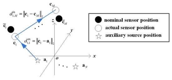
Figure 1.
The arrangement of the distributed sensor network assisted by N auxiliary sources.
Internal Measurement: Assuming all range measurements have been extracted from the received signals by sensors after a preprocessing algorithm, the internal range measurement from sensor l to sensor k, due to the line-of-sight propagation, is expressed by
where is the true internal propagation range and is the internal measurement noise. In practice, under the noise model in [38,39], the internal noise is modeled as zero-mean Gaussian with range-dependent variance , for the measurement noise relies on the SNR at each receiving end. Concatenating for yields
where , , and with . Furthermore, collecting the internal range measurements in for into a column vector yields
where and .
External Measurement: The external range measurement from auxiliary source n to sensor k can be expressible in the alternative form as
where is the true external propagation range and is the external measurement noise with range-dependent variance . Then, gathering the external range measurements from auxiliary source n into a column vector yields
where , , and with . Afterwards, stacking for obtains
where and .
We simplify range measurement as measurement hereafter for compactness. Then stacking (3) and (6) together yields
where the total measurement noise vector is zero-mean Gaussian with known noise covariance matrix
where the internal measurement noises are assumed statistically independent of external measurement ones.
In this work, the identifiability of sensor position perturbations under two cases is analyzed and the two cases are to be introduced in the following sections.
Case One, referred to as internal calibration, aims to refine the sensor positions with uncertainties via these internal measurements collected in , and all unknown parameters in Case One are arranged in
where , , and .
Case Two, called as external calibration, attempts to refine the sensor positions with uncertainties via jointly employing the internal and external measurements included in , where the unknown parameter set η is as same as that in (9).
3. Bayesian Cramer–Rao Lower Bound
3.1. The Expression of Bayesian Cramer–Rao Lower Bound
If all unknown parameters are random with available prior distribution, the BCRLB provides us a lower bound for the MSE of any estimator for these random parameters [9], e.g., the maximum a posteriori (MAP) estimator, and it is equal to the inverse of the Bayesian FIM (BFIM) created from the PDF of the underlying problem.
In accordance with Bayes’ rule [24], the logarithmic PDF, based on the measurements included in r and the prior information imposed on η, is
where p(r|η) is the conditional PDF of r given η and p(η) is the prior PDF of η with
and
In (11) and (12), K1 and K2 represent constants irrelevant of η, μ represents the mean vector of r with covariance matrix Σr, and Ση defines the covariance matrix of η. Inserting (11) and (12) into (10), applying partial derivatives w.r.t. the unknowns in η twice, negating the sign, and taking expectation in the sequel yield the BFIM as [5]
where and are components of describing, respectively, contributions of the measurements and prior statistics to the lower bound on the estimation error. For ease of description, we hereafter refer to as measurable FIM and as prior FIM. They are expressible in order as
and
Plugging (11) and (12) into (14) and (15) and implementing a few lines of algebra yield [40]
and
where size(η) denotes the length of η. From (16), we find that is Hermitian positive semidefinite, for it possesses a symmetrical structure and the covariance matrix Σr is positive definite. To emphasize, even though the measurement vector r is not Gaussian, [40] deduces that can still be written in the same structure as in (16) except for replacing with some positive definite matrix, provided that the term is continuous. Particularly, the positive definite matrix should be when r is Gaussian of the mean vector μ and covariance matrix Σr. So, the Gaussian hypothesis concerning the measurement vector r is not unreasonable.
3.2. The Asymptotical Tightness of Bayesian Cramer–Rao Lower Bound
Since we restrict our attention to the identifiability analysis of sensor position perturbations by using the BCRLB in the next section, we must prove the BCRLB is tight (or asymptotically tight) before we use it [23]. Otherwise, we may induce the erroneous results based on the BCRLB. Although it is difficult to judge the tightness of such a nonlinear model herein, one can determine the asymptotical tightness of the BCRLB through adopting the method in [28].
The assumption of small perturbations is considered here that the standard deviation σ is much smaller compared to the minimal internal/external range [9]. At this time, the averaging operation in of (13) appears trivial and the random Jacobian matrix Λ in (16) can be replaced in terms of its approximate version where all partial derivatives are simply evaluated at nominal sensor locations (η = 0) with [23]
From (18), it is deduced that the BCRLB is asymptotically tight under the assumption of small perturbations based on the method in [28]. Therefore, the BCRLB can serve as a benchmark to study the identifiability issue with the approximately following form:
4. Identifiability Analysis
With respect to [11], the random unknown parameters are convinced to be identifiable, only if the BCRLB approaches zero at sufficiently high SNRs and is tight, which means that these parameters can be estimated without error. Currently, all eigenvalues of the BFIM are proportional to SNRs, or equivalently, the BFIM behaves positive definite. From (13), when SNR is low, the prior FIM plays a major role in the BFIM and obviously it is positive definite by observing (17). However, when SNR grows large, the measurable FIM predominates in the BFIM. To guarantee parameter identifiability, apart from asymptotical tightness of the BCRLB confirmed in Section 3.2, the invertibility of the measurable FIM is still required, for the measurable FIM has been positive semidefinite owning to its symmetrical structure of (16). The following theorem is devoted to the link between invertibility of the measurable FIM (or rank of the Jacobian matrix) and the identifiability of perturbations, which can be used as a principle for the identifiability analysis. Note that the BFIM and the BCRLB play an identical role in the identifiability analysis, and they can be used interchangeably.
Theorem 1.
The perturbations in sensor positions of a distributed network become identifiable, if the Jacobian matrix concerning these perturbations has full row rank.
Proof of Theorem 1.
According to [40], the measurable FIM is of the form where the matrix W is positive definite regardless of the distribution concerning the measurement vector r. Here, the Gaussian noise hypothesis is assumed with the measurable FIM of (16) for analytical convenience. Note that the symmetric positive definite matrix can be divided via the Cholesky decomposition into where Lr is also positive definite. As and for any given nonsingular matrix B, we immediately yield [41,42];
As reported previously, if the measurable FIM is positive definite, the identifiability of sensor position perturbations can be guaranteed. As the measurable FIM possesses a symmetrical structure, its invertibility is still needed to ensure parameter identifiability, or equivalently, the Jacobian matrix Λ in (20) should have full row rank with
where denotes the row number of Λ. Note that the row number of the Jacobian matrix represents the number of unknown parameters in η and column number, notated by , is the number of measurements with the general relation . □
In the sequel, one central issue is to discover whenever the Jacobian matrix Λ has full row rank.
4.1. Case One: Internal Calibration
In Case One, there exist uncertainties in sensor positions of a distributed network to be estimated. On the occasion, substituting η in (9), , and into (16) creates
By introducing the transformation matrix
the internal Jacobian matrix P is further decomposed as
where
with representing the cosine value of the bearing angle of sensor l to sensor k w.r.t. the x axis,
with representing the cosine value of the bearing angle of sensor l to sensor k w.r.t. the y axis, and
with representing the cosine value of the bearing angle of sensor l to sensor k w.r.t. the z axis.
Then we restrict our attention to computation of rank[P]. It is evident from (24) and (25) that the elements of the internal Jacobian matrix P depend on geometrical factors, such as the number of sensors and network configuration. The determination of rank[P] is generally difficult. Nonetheless, we can introduce an auxiliary matrix Q with the relation rank[Q] = rank[P], of which the rank is much easier to obtain. It is primarily because the size dimensions of Q are generally no more than those of P.
Lemma 1.
Theauxiliary matrix
where
withand, satisfies
Proof of Lemma 1.
Since the rank of a matrix cannot exceed either of its size dimensions [42], we have
Invoking the matrix
yields
which holds because , see [42]. Combining (29) and (31) immediately has
Substitution of (25a) into (24) yields
Since HT1M = 0, we deduce that
Incorporating (32), one deduces that
It is easily discovered that any M − 1 rows of H are linearly independent, and hence a full row rank matrix can be obtained through deleting any one row of H.
On the other hand, the propagation symmetry from sensors to sensors implies that the number of nonrepetitive columns in the internal Jacobian matrix P, i.e., ρnp(P), is reduced by half, like with
Then based on (35) and (36), we design the transformation form
where and
to delete the linear correlated row and repetitive columns in Px. Applying (24) and (38) into (37) yields
As a full row rank matrix can be constructed by deleting any one row of Px, we use the transformation matrix L to remove the first row of Px. The matrix R aims to eliminate the repetitive columns in Px. Analogously, we have Qy = LPyRT and Qz = LPzRT, leading to the establishment of the auxiliary matrix . Noting that the matrix rank is irrelevant of linear correlated rows and repetitive columns, Lemma 1 is thus proved. □
With the auxiliary matrix Q in hand, the following lemma is confined to the acquisition of rank[Q].
Lemma 2.
For any adopted nominal sensor network other than the collinear and coplanar geometries, the term rank[Q] is
Proof of Lemma 2.
See Appendix A. □
It also indicates that rank[Q] equals to M − 1 for the nominal collinear sensor geometry and to 2M − 3 for the nominal coplanar sensor geometry [9].
Combining (20), (28), and (40) produces
which violates (21) and further the invertibility of . After eigenvalue decomposition, possesses an eigenvalue 0 of multiplicity and positive eigenvalues with [42]
where
Λ1 is a diagonal matrix with positive eigenvalues of on its diagonal and U1 is the matrix of relevant eigenvectors. U2 is the matrix of the eigenvectors concerning all zero eigenvalues. Since all the positive eigenvalues are proportional to SNRs, one arrives at
As the BCRLB is asymptotically tightly proved in Section 3.2, it, by invoking (17), (19), and (42)–(44), can be given by
When SNR tends to infinity, (46) turns to
Therefore, adding the prior statistical information of sensor position perturbations, which does not vary with SNR, is expected to result in a constant error in the form of the BCRLB as SNR tends to infinity. As a result, in the case of internal calibration, when no true sensor positions are available, the measurable FIM remains always singular, leading to unidentifiability of all sensor position perturbations. Currently, the sensor network is observable from these internal measurements up to rotation and translation.
Remark 1.
From (41), the self-localization of sensor networks seems feasible if there exist six parameters in η to be assumed known previously. Currently, an invertible measurable FIM is obtainable by removing the rows and columns in that correspond to the six assumed known parameters. A detailed analysis in Appendix A gives us a possible set of the six parameters, which is
The first three quantities in (48) determine the reference position of the sensor network, and in reality, the reference position can choose any one of sensor positions as well. The derivations in Appendix A also indicate that the remaining three ones in (48) cannot be from the identical sensor or identical axis; otherwise, the measurable FIM, which is obtained via removing the rows and columns in that relate to the assumed known parameters, would still be singular. Hence, in the case of internal calibration, the identifiability condition for self-calibration of sensor position perturbations in 3-D space is given that, the precise knowledge of the position of one sensor and orientation to a second sensor in addition to the coordinate of a third sensor along some axis is required.
4.2. Case Two: External Calibration
When no accurate knowledge of sensor positions is available, the obvious method is to introduce calibrating sources for efficient calibration, e.g., several auxiliary sources in known locations. In this section, we focus on estimating all sensor position perturbations through jointly using the internal and external measurements. Later, application of η in (9), , and into (16) yields
with the internal Jacobian matrix defined in (24) and external Jacobian matrix of the following form
where
with denoting the cosine value of the bearing angle of source n to sensor k w.r.t. the x axis,
with denoting the cosine value of the bearing angle of source n to sensor k w.r.t. the y axis, and
with denoting the cosine value of the bearing angle of source n to sensor k w.r.t. the z axis.
Some procedures analogous to the last section provide an auxiliary matrix , whose size dimensions are no more than those of U, with the relation rank[W] = rank[U] and with the matrix R defined in (38).
Now we confine our attention to the calculation of rank[W]. As reported in Theorem 1, assuming the column number is no less than the row number for a Jacobian matrix, the rank of the Jacobian matrix should equal the number of unknown parameters in η according to (21), to ensure identifiability of sensor position perturbations, i.e., [16]
Recalling from Lemma 2, to warrant (52), rank[S] should satisfy
which holds because for any given matrix , see [42]. When the number of sensors is no less than four, the column number of S requires
from which it seems that the required source number N can be arbitrarily small with a sufficiently large M. Later, we shall demonstrate that perturbations in all sensor positions become identifiable in the presence of at least three noncollinear auxiliary sources, with the nominal collinear and coplanar sensor geometries ruled out.
Lemma 3.
For any adopted nominal sensor network other than the collinear and coplanar geometries, the term rank[W] is
Proof of Lemma 3.
Due to [42], the homogeneous system WTγ = 0 has a unique solution—the trivial solution γ = 0, if and only if WT has full column rank; at this time, the identifiability of sensor position perturbations can be completed. It proceeds to find out the condition under which the homogeneous system can have the unique trivial solution. Substituting W = [PRT, S] into WTγ = 0 yields the internal system RPTγ = 0 and the external one STγ = 0. The vector
where , , and . It is noted that the goal of dividing γ into three parts in (56) is to achieve the consistency between partitions of the vector γ and of Jacobian matrices in W. The first two lines of (55) have been verified in Appendix B and then we try to acquire rank[W] when . □
4.2.1. The Sensor-Source Configuration to Insure rank[S] = 3M
Substituting (50) and (56) into the external system STγ = 0 gives rise to
Rearranging all the equations in (57) generates the following M groups of equations
from which we can find that the position of each sensor can be computed independently of the other sensors.
When the number of sources satisfies N = 3 with a noncollinear geometry, the coefficient matrix inside the first bracket at the left-hand side of (58) (called as the kth coefficient matrix) has full column rank, provided that any pair of sources is noncollinear w.r.t. sensor k, . For instance, given some k, if or holds for some pair of sources , , the kth coefficient matrix would be rank-deficient, as expected in Figure 2a, where the pair of source 1 and source 2 is collinear w.r.t sensor k.
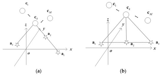
Figure 2.
The source geometries (N = 3) for (a) inducing the kth coefficient matrix rank-deficient and (b) inducing the singularity of all coefficient matrices.
As depicted in Figure 2b, among three sources, although any pair of sources is noncollinear w.r.t. sensor k, all these sources lie in a straight line, inducing that all the M coefficient matrices in (58) are rank-deficient.
If all the M coefficient matrices in (58) have full column rank, we conclude that the external system STγ = 0 has the unique trivial solution [42], indicating the matrix S is full row rank with rank[S] = 3M. Note that
Combining rank[S] = 3M with (59) immediately yields
The nearest equation insures the identifiability of sensor position perturbations. At this time, it requires that the three sources should avoid collinear geometry, and among them, any pair of sources should be noncollinear w.r.t. each sensor.
In a similar manner, when the number of auxiliary sources exceeds three, for the purpose of parameter identifiability, it demands that as for each sensor, there should exist at least three noncollinear auxiliary sources and among them any pair of sources should be noncollinear w.r.t. the sensor.
Figure 3 provides us an example of non-coplanar source geometry with the presence of four sources. When source 4 lies in point a, all four sources are in a plane. There always exist three noncollinear sources but among them not all pairs of sources are noncollinear w.r.t. sensor k. For example, in the noncollinear geometry of sources 1, 2, and 4, the pair of source 1 and source 2 is collinear w.r.t. sensor k, thereby leading to a rank-deficient matrix S. When source 4 is moved from point a to point b, a non-planar source geometry occurs. It is obvious that there must exist three noncollinear sources and among them any pair of sources is noncollinear w.r.t. each sensor, leading to a full row rank matrix S and further a full row rank matrix W. Hence, when the number of sources exceeds three, a non-coplanar source geometry automatically relates to the full row rank matrices S and W. At this time, accurate configuration calibration can be made by using external measurements only.
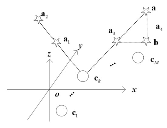
Figure 3.
The coplanar and non-coplanar source geometries (N = 4).
4.2.2. The Sensor-Source Configuration to Insure rank[W] = 3M
The last subsection makes sensor position perturbations identifiable through letting the external Jacobian matrix S full row rank, which can further lead to a full row rank matrix W. However, although S is rank-deficient, the identifiability of sensor position perturbations may also be completed if W is full row rank with rank[W] = 3M. Accordingly, the requirements concerning source geometries in the last subsection may appear relatively rigorous. Some geometries may not lead to a full row rank matrix S but can relate to a full row rank matrix W, and further, the identifiability can be achieved. Concurrently, accurate configuration calibration can be completed via jointly using all internal and external measurements.
As stated in Lemmas 1 and 2, we present
Noting that V is obtained by deleting the repetitive columns in the internal Jacobian matrix P, we conclude that the two homogeneous systems VTγ = 0 and PTγ = 0 share the identical general solution. As a result, invoking (A5) in Appendix A obtains all the free variables in the general solution of the system VTγ = 0 as
It means that, to make all the unknowns identifiable, at least six equations should be provided by the external system STγ = 0 in (57) to determine the six free variables in (62). Like (A3) in Appendix A, all basic variables in the general solution of the system WTγ = 0 are linear functions of free variables and once all free variables are uniquely determined, all basic variables can then be uniquely fixed. From [42], the system WTγ = 0 thus can have the unique trivial solution, meaning that W is full row rank.
As proved in Appendix B, the unidentifiability of sensor position perturbations occurs in the presence of less than three auxiliary sources and the six free variables in (62) relate to three sensors with the indices 1, M − 1, M, indicating the six equations provided by the external system must come from three sources and three sensors. So, for example, the six equations from the external system can be chosen as
where the first three equations are devoted to the acquisition of the first three free variables and the other three resort to the obtainment of the remaining three free variables in (62).
If sources 1, 2, and 3 are noncollinear and among them any pair of sources is noncollinear w.r.t. sensor 1, solving the first three equations in (63) has . Later, the other three equations in (63) are functions of the remaining three free variables , , and . When the pair of source 1 and 2 is noncollinear w.r.t. sensor M, the remaining three free variables are determined uniquely with from the other three equations in (63). Back substituting the six free variables into all the 3(M − 2) basic variables yields the unique trivial solution γ = 0, which reflects that the matrix W is full row rank.
Currently, the minimal number of three noncollinear auxiliary sources is required with the collinear and coplanar sensor geometries ruled out for the confidence of the applicability of (61). So, Lemma 3 is proved. □
According to the identifiability conditions given in Section 4.2.1 and Section 4.2.2, the geometries in Figure 2a and Figure 3 where source 4 is at point a form a full row rank matrix W without the presence of a full row rank matrix S, leading to the identifiability of sensor position perturbations. Hence, more available geometries are included in this subsection (Section 4.2.2) than in the last subsection (Section 4.2.1).
From Lemma 3, it is implied that the identifiability of sensor position perturbations can be made with the required minimal amount of three noncollinear auxiliary sources, where the nominal collinear and coplanar sensor geometries should be excluded. When the number of auxiliary sources is less than three, the intrinsic ambiguity problem incurs and further results in the parameter unidentifiability.
Referring to Theorem 1, once the Jacobian matrix U has full row rank with rank[U] = rank[W] = 3M, the measurable FIM behaves positive definite. All the eigenvalues of the measurable FIM are larger than zero and proportional to SNRs. Furthermore, when SNR approaches infinity, the BCRLB, by invoking the eigenvalue decomposition of the BFIM, becomes
which represents that the estimation accuracy of perturbations is only limited by SNRs.
Remark 2.
Using the matrix inversion formula in [43], the BCRLB can also be delivered by
wherebehaves positive definite. It is noteworthy that the first term in the second line of (65) represents the BCRLB in the absence of internal measurements. The second term in the second line of (65) is the performance improvement due to the involvement of internal measurements, which is a positive semidefinite matrix by observing its symmetric structure and the internal Jacobian matrixPbeing rank-deficient.
Remark 3.
By observing the structures of the internal and external Jacobian matrices, the external calibration in a M-sensor network with the assistance of N auxiliary sources is equivalent to the internal calibration in a -sensor network, among which the locations of N sensors have been well-estimated previously in terms of the Jacobian matrix perspective.
Remark 4.
When one auxiliary source is used, there should know three quantities inηof (9) to guarantee the identifiability of remaining sensor position perturbations due to Lemma 3. As the auxiliary source and assumed known sensor contribute in an equivalent fashion to calibration, the three quantities should come from two distinct sensors according to the second line of (55) in Lemma 3. When two auxiliary sources are introduced, there should know a perturbation parameter inηto achieve the identifiability of remaining sensor position perturbations.
5. Simulation Results
In this section, some numerical simulations are conducted to evaluate the effectiveness of this work. From the practical point of view, since the standard derivation of each measurement noise depends on the SNR at the receiving end, it can be thus represented as [38,39]
where R = 104 m is the radius of the surveillance area and α is a constant depending on transmitting power and noise level. It should be noted that the parameter α is inversely proportional to SNR. The normalization factor R is used to make α a parameter with meter unit. Denote the root mean BCRLB (RMBCRLB) as
5.1. Scenario 1: The Asymptotical Tightness of the BCRLB
Due to (18), the asymptotical tightness of the BCRLB is completed analytically under the assumption of small sensor position perturbations, leading to the approximation The approximate and accurate RMBCRLBs have the similar form as in (67) except that the term in the accurate RMBCRLB is replaced by another term in the approximate version. To confirm the correctness of the approximation, the accurate RMBCRLB is plotted in Figure 4 with its approximate form provided for comparison, where the internal calibration scenario of a three-sensor network is assumed with . So, all the unknowns in η in this case are identifiable, for the identifiability condition in Remark 1 is met. The sensors are nominally placed with azimuth and elevation angles uniformly distributed in [0, 2π) and [π/10, π/2] respectively, along the surface of a globe with radius 103 m.
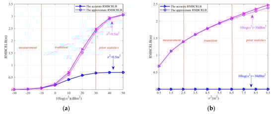
Figure 4.
The RMBCRLB for configuration calibration versus 10log(α2) and σ2 in the case of internal calibration. (a) The RMBCRLB versus 10log(α2) under different σ2. (b). The RMBCRLB versus σ2 under different 10log(α2).
It is observed from Figure 4a,b that the RMBCRLB curve can be divided into three sections, i.e., prior statistics section, transition section, and measurement section. In the prior statistics section, the RMBCRLB primarily relies on the prior statistical information of sensor position perturbations, and it grows large with increasing σ2, since 10log(α2) is large and the measurements are unreliable. In the measurement section, the RMBCRLB mainly depends on the received data and seems irrelevant to σ2, since 10log(α2) is small enough. The transition section is between the two sections. It is found from Figure 4b that the smaller the parameter 10log(α2), the more slowly the accurate RMBCRLB deviates from its approximate version as the variance σ2 increases. It is because the RMBCRLB grows large with increasing σ2 at large 10log(α2) where dominates and the RMBCRLB is constant as σ2 increases at small 10log(α2) where dominates. Inspection of Figure 4b provides that the deviation between the accurate and approximate RMBCRLBs occurs in the prior statistics section. It seems that the larger the variance σ2, the more the deviation between the accurate and approximate RMBCRLBs. As a result, the accurate RMBCRLB gradually degenerates to the approximate form when 10log(α2) or σ2 is small enough, which verifies asymptotical tightness of the BCRLB under the assumption of small sensor position perturbations.
5.2. Scenario 2: The Effect of the Number of Auxiliary Sources and Sensors on Internal and External Calibration
The impact of number of auxiliary sources and sensors on the RMBCRLB for configuration calibration is examined in Figure 5. The placement of all sensors is kept the same as in Figure 4. The heights of all auxiliary sources are uniformly distributed in [100, 500] m. Projecting all auxiliary sources on the ground yields a circle of radius 103 m with the circle point being the origin of Cartesian coordinates. Here, the case of external calibration A employs all internal and external measurements jointly to calibrate perturbations in all sensor positions while the case of external calibration B uses external measurements only. The case of internal calibration exploits internal measurements to calibrate perturbations in all sensor positions. It is apparent from Figure 5a,b that the case of external calibration A outperforms the remaining cases regardless of the chosen parameter 10log(α2), for all internal and external measurements are properly used. The RMBCRLB improves as the number of sensors and auxiliary sources grows large in this case. From Figure 5b, we see that the RMBCRLB in the case of internal calibration improves as the number of sensors increases. However, as previously derived in Section 4.1, perturbations in all sensor positions become unidentifiable without the aid of auxiliary sources and hence, the RMBCRLB in this case converges to a constant error at high SNRs or small 10log(α2)s, as expected in Figure 5b. The RMBCRLB in the case of external calibration B is nearly unaffected by the number of sensors and only improves with the amount of auxiliary sources, for only external measurements are employed.
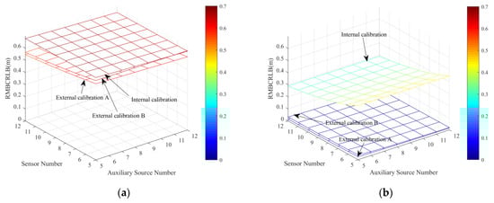
Figure 5.
The RMBCRLBs for configuration calibration versus the number of auxiliary sources and sensors with σ2 = 0.5 m2 under different transmitting power parameters. (a) 10log(α2) = 30 dBm2. (b) 10log(α2) = −10 dBm2.
5.3. Scenario 3: The Identifiability of External Calibration
The identifiability condition in Lemma 3 is verified in Figure 6, in which the nominal placement of sensors is kept the same as in Figure 4 except for the number of sensors M = 6 here. The variance of sensor position perturbations is set as σ2 = 0.5m2. The source placement is as same as that in Figure 5. We observe from Figure 6 that when N < 3, the RMBCRLB approaches a constant as 10log(α2) decreases. When , the RMBCRLB can be reduced to an arbitrarily small amount at sufficiently small 10log(α2)s, or equivalently, sensor position perturbations are identifiable. In addition, all the curves of external calibration A possess a higher accuracy than their counterparts of external calibration B. We would like to clarify that, although the identifiability can be guaranteed using external measurements only, the involvement of internal measurements enables additional information to calibration. It should not degrade, if not improve, the calibration accuracy when internal measurements are used properly. Inspection of Figure 6a asserts that, at a small 10log(α2), the RMBCRLB decreases with increasing the number of auxiliary sources N. However, the improvement rate gradually decreases when the number of auxiliary sources N increases to more than 4. The result in Remark 3 is confirmed in Figure 6b, where M’ is defined to be the number of assumed known sensors in the network. The conclusion from Figure 6b is similar to that in Figure 6a.
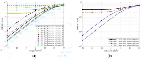
Figure 6.
The RMBCRLBs for configuration calibration versus 10log(α2) under different numbers of auxiliary sources and of assumed known sensors when σ2 = 0.5m2. (a) The RMBCRLBs versus 10log(α2) under different numbers of auxiliary sources. (b) The RMBCRLBs versus 10log(α2) under different numbers of assumed known sensors.
5.4. Scenario 4: The Advantage of Introducing Internal Measurements
Consider configuration calibration of a six-sensor non-coplanar network with the aid of three noncollinear auxiliary sources. Here, the definitions of external calibration A and B are identical to those in Figure 5. The sensor-source configuration is depicted in Figure 7a where blue circles represent auxiliary source positions and green stars nominal sensor positions. It can be observed that a collinear geometry exists among sensor 1, sensor 2, sensor 3, source 1, and source 2. At this time, the pair of source 1 and source 2 is collinear w.r.t. any one of the three sensors, i.e., sensor 1, sensor 2, and sensor 3. Hence, such a sensor-source configuration leads to a rank-deficient external Jacobian matrix according to the derivations in Section 4.2.1, which reflects that the configuration calibration of any desired accuracy cannot be made through using external measurements only under the configuration in Figure 7a. However, when the joint use of internal and external measurements is considered, the identifiability condition in Section 4.2.2 is guaranteed in such a configuration of Figure 7a. Concurrently, all sensor position perturbations can be estimated without error when all internal and external measurements are used simultaneously, as depicted in Figure 7b. As a result, the configuration calibration of jointly using internal and external measurements can contain more available source geometries than that of using external measurements only. Additionally, the external calibration A can yield a higher positioning accuracy than the external calibration B.
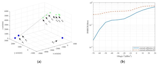
Figure 7.
The RMBCRLBs for configuration calibration versus 10log(α2) with/without the presence of internal measurements when σ2 = 0.5 m2. (a) The arrangement of the distributed sensor network assisted by three noncollinear auxiliary sources. (b) The RMBCRLBs versus 10log(α2) with/without the presence of internal measurements.
6. Discussion
This work studies the parameter identifiability condition for configuration calibration in a 3-D distributed sensor network with and without the presence of several auxiliary sources in known locations. The analysis indicates that, although the utilization of internal measurements fails to accomplish entire configuration calibration of any desired accuracy, they can be properly applied into external calibration for enhancing positioning accuracy. The involvement of internal measurements is able to relax the requirement on the source placement compared to the neglect of internal measurements. The parameter identifiability condition for joint sensor positions and velocities estimation in a distributed network is our future work.
Until now, we have primarily focused on the establishment of theoretical models and performance assessment of numerical simulations. We evaluate the BCRLB performance of configuration calibration through the MATLAB tool from several aspects, such as the tightness of BCRLB, number of sensors and auxiliary sources, and advantage of using internal measurements. But regretfully, we have no access to the obtainment of the actual data and establishment of a real-life system. The transition from theory to practice is our future goal.
7. Conclusions
In this work, the identifiability of sensor position perturbations in a distributed network is explored by establishing the link between the rank of the Jacobian matrix and parameter identifiability under Gaussian noise. Since the asymptotical tightness of the BCRLB for configuration calibration under the assumption of small sensor position perturbations is verified, we may use the BCRLB to measure the identifiability. It indicates that all sensor position perturbations appear unidentifiable in the case of internal calibration. The analysis also delivers the identifiability condition for the case of partly internal calibration, that the knowledge of the location of a sensor and orientation to a second sensor in addition to the coordinate of a third sensor along some axis is required. In the case of external calibration, the identifiability of all sensor position perturbations requires the minimal amount of three noncollinear auxiliary sources with the nominal collinear and coplanar sensor geometries ruled out. In the case of external calibration, although the involvement of internal measurements does not change the required minimum of auxiliary sources, it can contain more available source geometries and provide higher calibration accuracy compared to the neglect of internal measurements.
Author Contributions
Conceptualization, X.L.; methodology, X.L.; software, X.L.; formal analysis, X.L.; data curation, X.L.; writing—original draft preparation, X.L.; validation, T.W.; visualization, T.W.; investigation, J.C.; supervision, J.C. All authors have read and agreed to the published version of the manuscript.
Funding
This research was supported by the National Key R&D Program of China (Grant No. 2021YFA1000400).
Data Availability Statement
Not applicable.
Acknowledgments
The authors would like to thank the editor and anonymous reviewers for their helpful comments and suggestions.
Conflicts of Interest
The authors declare no conflict of interest.
Appendix A
To obtain the matrix rank, the matrix nullity is invoked, using the rank plus nullity theorem [44], yielding
where defines the dimension of the nullspace
Then, one resorts to the general solution of the homogeneous system QTγp = 0. As Q is of the form , it is innocuous to divide the unknown vector γp into for the consistency between partitions of Q and of γp where , , and . It should be emphasized that the subscripts of all the variables in begin with the index 2, for Qx = LPxRT is obtained through removing the first row of Px which relates to sensor 1, due to Lemma 1. So do and . After a few lines of algebra including Gaussian elimination [44], the general solution for the system QTγp = 0 is
where h1 is the 3(M − 1) × 1 special solution vector when , , and are respectively equal to 1, 0, and 0. Similarly, h2 and h3 are also special solution vectors and the three special solution vectors are linearly independent with one another [44].
Through observing the general solution in (A3), we can observe that all unknown variables in γp can be expressible in terms of , , and . Referring to [42], in the general solution of a homogeneous system, some unknown variables, named basic variables, can be expressed in terms of the other unknown variables, whose values remain arbitrary, and consequently the arbitrary unknown variables are referred to as free variables. As a result, there are 3(M − 2) basic variables and 3 free variables in (A3). Since the three free variables can range over all possible values, (A3) describes all possible solutions.
h1, h2, and h3 are linearly independent, leading to a basis {h1, h2, h3} for the nullspace of QT. As the dimension of the nullspace is equal to the number of vectors in a basis spanning the nullspace, it follows from (A3) that
(A4) holds for any adopted nominal sensor network other than the collinear and coplanar geometries. Some derivations conclude that the rank of QT equals to M − 1 for the nominal collinear sensor geometry and to 2M − 3 for the nominal coplanar sensor geometry [9].
Moreover, since the auxiliary matrix Q is formed via removing three linear correlated rows in the internal Jacobian matrix P, which correspond to the unknown perturbations ∆x1, ∆y1, and ∆z1. If we resort to the general solution of the homogeneous system PTγ = 0 where with and , the number of free variables in the general solution of the system PTγ = 0 would be six, which are, respectively,
This is because the three linear correlated rows relating ∆x1, ∆y1, and ∆z1 in P may be expressed as a linear combination of the other rows. From [44], for a homogeneous system PTγ = 0, the columns of PT can be divided into basic and non-basic columns. The basic columns are the ones multiplied by basic variables and non-basic columns are the ones by free variables, in which the non-basic columns can be expressed as a linear combination of the basic columns. Once these six free variables are determined uniquely, all basic variables in γ can be fixed subsequently. Precisely, when the perturbations, which correspond to the free variables in (A5), i.e.,
are assumed known, all the special solution vectors vanish in the general solution of the system PTγ = 0 and we have γ = 0. A full row rank Jacobian matrix is obtainable through removing the rows of P corresponding to the six assumed known variables in (A6).
Appendix B
(1) N = 1
Through observing structures of the internal Jacobian matrix in (24), (25) and the external Jacobian matrix in (50), (51), we see that the external calibration in a M-sensor network assisted by an auxiliary source is equivalent to the internal calibration in a M + 1-sensor network where the location of a sensor is accurately known in terms of the Jacobian matrix perspective. Currently, by invoking Lemma 2, we directly have
which reflects all sensor position perturbations are unidentifiable in a M-sensor network with the presence of one auxiliary source.
(2) N = 2
By invoking (A1), the matrix rank can be obtained using the rank plus nullity theorem. Analogously, to cast rank[W], one attempts to solve for the general solution of the homogeneous system WTγ = 0 and the nullity null[WT] is equal to the number of free variables in the general solution of the system [42], where γ has been defined previously in (56). Since the system WTγ = 0 can be decomposed into internal and external systems, we firstly expand the external system STγ = 0 by using (50) and (56) as
Solving (A8) gives
where
The sensor-source configuration forbids (A9) and (A10) if or for any given k. Besides, (A10) requires for each k.
Later, the internal system RPTγ = 0, by invoking (24), (56), and (A9), turns to
where .
Then, moving the first column of the matrix D, which would be multiplied by in (A11), from the left-hand side to the right hand side of (A11), turns to
where contains all the other columns of D except for the first column included by . The matrix can be decomposed into where the upper block incorporates the first M − 1 rows of and lower block the remaining rows of . After applying (A9) and (A10) into and doing some mathematical simplifications, the upper block becomes
which is nonsingular as long as (A9) and (A10) hold. Moreover, as the matrix rank cannot exceed either of its size dimensions with [42]
has full column rank provided that with
Thus, the number of sensors should satisfy under this setting. Based on the least square estimation [44], the vector in (A12) can be computed uniquely as
Until now, the general solution of the system WTγ = 0, by combining (A9) with (A16), can be generated as
from which we can see that the unknown is the only free variable. As a result, (A17) is a basis for the nullspace N(WT) and according to the rank plus nullity theorem [42], it follows
References
- Schultheiss, P.M.; Ianniello, J.P. Optimum range and bearing estimation with randomly perturbed arrays. J. Acoust. Soc. Am. 1980, 68, 167–173. [Google Scholar] [CrossRef]
- Ho, K.C.; Lu, X.; Kovavisaruch, L. Source Localization Using TDOA and FDOA Measurements in the Presence of Receiver Location Errors: Analysis and Solution. IEEE Trans. Signal Process. 2007, 55, 684–696. [Google Scholar] [CrossRef]
- Sun, B.; Zhang, X.; Liao, D.; Li, X. Target localization sensitivity using MIMO radar in the presence of antenna position uncertainties. In Proceedings of the 8th IEEE Sensor Array Multichannel Signal Processing Workshop (SAM), Coruna, Spain, 22–25 June 2014; pp. 509–512. [Google Scholar] [CrossRef]
- Moses, R.L.; Patterson, R. Self-calibration of sensor networks. In Proceedings of the SPIE 4743, Unattended Ground Sensor Technologies and Applications IV, Orlando, FL, USA, 2–5 April 2002; Volume 4743, pp. 108–119. [Google Scholar]
- Liu, X.; Wang, T.; Chen, J.; Wu, J. Efficient configuration calibration using ground auxiliary receivers at inaccurate locations. Digit. Signal Process. 2022, 129, 103675. [Google Scholar] [CrossRef]
- Sun, M.; Yang, L.; Ho, K. Accurate sequential self-localization of sensor nodes in closed-form. Signal Process. 2012, 92, 2940–2951. [Google Scholar] [CrossRef]
- Ashok, E.; Schultheiss, P. The effect of an auxiliary source on the performance of a randomly perturbed array. In Proceedings of the IEEE International Conference on Acoustics, Speech, & Signal Processing, San Diego, CA, USA, 19–21 March 1984. [Google Scholar]
- Yang, L.; Ho, K.C. Alleviating Sensor Position Error in Source Localization Using Calibration Emitters at Inaccurate Locations. IEEE Trans. Signal Process. 2010, 58, 67–83. [Google Scholar] [CrossRef]
- Rockah, Y.; Schultheiss, P. Array shape calibration using sources in unknown locations--Part I: Far-field sources. IEEE Trans. Acoust. Speech Signal Process. 1987, 35, 286–299. [Google Scholar] [CrossRef]
- Rockah, Y.; Schultheiss, P.M. Array shape calibration using sources in unknown locations-Part II: Near-field sources and es-timator implementation. IEEE Trans. Acoust. Speech Signal Process. 1987, 35, 724–735. [Google Scholar] [CrossRef]
- Wan, S.; Tang, J.; Zhu, W.; Zhang, N. Identifiability Analysis for Array Shape Self-Calibration Based on Hybrid Cramér-Rao Bound. IEEE Signal Process. Lett. 2014, 21, 473–477. [Google Scholar] [CrossRef]
- Zhang, N.; Tang, J.; Wan, S.; Tang, X. Identifiability analysis for array shape self-calibration in MIMO radar. In Proceedings of the IEEE Radar Conference, Cincinnati, OH, USA, 19–23 May 2014; pp. 1108–1113. [Google Scholar]
- Lu, J.; Liu, F.; Sun, J.; Miao, Y.; Liu, Q. Multi-Target Localization of MIMO Radar with Widely Separated Antennas on Moving Platforms Based on Expectation Maximization Algorithm. Remote Sens. 2022, 14, 1670. [Google Scholar] [CrossRef]
- Lu, J.; Liu, F.; Sun, J.; Liu, Q.; Miao, Y. Joint Estimation of Target Parameters and System Deviations in MIMO Radar With Widely Separated Antennas on Moving Platforms. IEEE Trans. Aerosp. Electron. Syst. 2021, 57, 3015–3028. [Google Scholar] [CrossRef]
- Amiri, R.; Behnia, F.; Noroozi, A. An Efficient Estimator for TDOA-Based Source Localization with Minimum Number of Sensors. IEEE Commun. Lett. 2018, 22, 2499–2502. [Google Scholar] [CrossRef]
- Noroozi, A.; Sebt, M.A.; Hosseini, S.M.; Amiri, R.; Nayebi, M.M. Closed-Form Solution for Elliptic Localization in Distributed MIMO Radar Systems with Minimum Number of Sensors. IEEE Trans. Aerosp. Electron. Syst. 2020, 56, 3123–3133. [Google Scholar] [CrossRef]
- Tomic, S.; Beko, M.; Tuba, M.; Correia, V.M.F. Target Localization in NLOS Environments Using RSS and TOA Measurements. IEEE Wirel. Commun. Lett. 2018, 7, 1062–1065. [Google Scholar] [CrossRef]
- Tomic, S.; Beko, M. A Geometric Approach for Distributed Multi-Hop Target Localization in Cooperative Networks. IEEE Trans. Veh. Technol. 2020, 69, 914–919. [Google Scholar] [CrossRef]
- Yang, Y.; Zheng, J.B.; Liu, H.W.; Ho, K.C.; Chen, Y.Q.; Yang, Z.W. Optimal sensor placement for source tracking under synchronization offsets and sensor location errors with distance-dependent noises. Signal Process. 2022, 193, 108399. [Google Scholar] [CrossRef]
- Nguyen, N.H.; Dogancay, K. Optimal Geometry Analysis for Multistatic TOA Localization. IEEE Trans. Signal Process. 2016, 64, 4180–4193. [Google Scholar] [CrossRef]
- Sadeghi, M.; Behnia, F.; Amiri, R. Optimal sensor placement for 2-D range-only target localization in constrained sensor geometry. IEEE Trans. Signal Process. 2020, 68, 2316–2327. [Google Scholar] [CrossRef]
- He, Q.; Blum, R.S. Cramer–Rao Bound for MIMO Radar Target Localization with Phase Errors. IEEE Signal Process. Lett. 2009, 17, 83–86. [Google Scholar] [CrossRef]
- Sun, P.L.; Tang, J.; Wan, S.; Zhang, N. Identifiability analysis of local oscillator phase self-calibration based on hybrid Cra-mér-Rao bound in MIMO radar. IEEE Trans. Signal Process. 2014, 62, 6016–6031. [Google Scholar] [CrossRef]
- Papoulis, A.; Pillai, S.U. Probability, Random Variables, and Stochastic Processes; Mc Graw-Hill International Book Co.: New York, NY, USA, 2002. [Google Scholar]
- Arafa, A.; Messier, G.G. A Gaussian model for dead-reckoning mobile sensor position error. In Proceedings of the IEEE 72nd Vehicular Technology Conference-Fall, Ottawa, ON, Canada, 6–9 September 2010; pp. 1–5. [Google Scholar]
- Zekavat, R.; Buehrer, R.M. Handbook of Position Location: Theory, Practice, and Advances; Wiley: Hoboken, NJ, USA, 2019. [Google Scholar]
- Messer, H. The hybrid Cramer-Rao lower bound-From practice to theory. In Proceedings of the 4th IEEE Sensor Array Mul-tichannel Signal Processing Workshop (SAM), Waltham, MA, USA, 12–14 July 2006; pp. 304–307. [Google Scholar]
- Tabrikian, J.; Krolik, J. Theoretical performance limits on tropospheric refractivity estimation using point-to-point microwave measurements. IEEE Trans. Antennas Propag. 1999, 47, 1727–1734. [Google Scholar] [CrossRef]
- Noam, Y.; Messer, H. Notes on the Tightness of the Hybrid CramÉr–Rao Lower Bound. IEEE Trans. Signal Process. 2009, 57, 2074–2084. [Google Scholar] [CrossRef]
- Lo, J.-H.; Marple, S. Observability conditions for multiple signal direction finding and array sensor localization. IEEE Trans. Signal Process. 1992, 40, 2641–2650. [Google Scholar] [CrossRef]
- Jauffret, C.; Barrere, J.; Chabriel, G. Array Shape Observability from Time Differences of Arrival. IEEE Trans. Aerosp. Electron. Syst. 2011, 47, 1515–1520. [Google Scholar] [CrossRef]
- Chung, P.J.; Wan, S. Array self-calibration using SAGE algorithm. In Proceedings of the 5th IEEE Sensor Array Multichannel Signal Processing Workshop (SAM), Darmstadt, Germany, 21–23 July 2008; pp. 165–169. [Google Scholar]
- Zhang, X.J.; He, Z.S.; Zhang, X.P.; Yang, Y. DOA and phase error estimation for a partly calibrated array with arbitrary geometry. IEEE Trans. Aerosp. Electron. Syst. 2020, 56, 497–511. [Google Scholar] [CrossRef]
- Ho, K.C.; Yang, L. On the Use of a Calibration Emitter for Source Localization in the Presence of Sensor Position Uncertainty. IEEE Trans. Signal Process. 2008, 56, 5758–5772. [Google Scholar] [CrossRef]
- Willerton, M.; Manikas, A. Array shape calibration using a single multi-carrier pilot. In Proceedings of the Sensor Signal Processing for Defence (SSPD 2011), London, UK, 27–29 September 2011; pp. 1–6. [Google Scholar]
- Aoki, S.; Tanji, H.; Murakami, T. Array shape calibration using near field pilot sources with unknown distance. In Proceedings of the 2017 Asia-Pacific Signal and Information Processing Association Annual Summit and Conference (APSIPA ASC), Kuala Lumpur, Malaysia, 12–15 December 2017; pp. 892–896. [Google Scholar]
- Ng, B.C.; Nehorai, A. Active array sensor location calibration. In Proceedings of the IEEE International Conference on Acoustics, Speech, & Signal Processing, Minneapolis, MN, USA, 27–30 April 1993; pp. 21–24. [Google Scholar]
- Amiri, R.; Behnia, F.; Zamani, H. Asymptotically Efficient Target Localization from Bistatic Range Measurements in Distributed MIMO Radars. IEEE Signal Process. Lett. 2017, 24, 299–303. [Google Scholar] [CrossRef]
- Willis, J.N. Bistatic Radar; SciTech: Raleigh, NC, USA, 2005. [Google Scholar]
- Jauffret, C. Observability and fisher information matrix in nonlinear regression. IEEE Trans. Aerosp. Electron. Syst. 2007, 43, 756–759. [Google Scholar] [CrossRef]
- Liu, X.; Wang, T.; Chen, J.; Wu, J. Efficient Configuration Calibration in Airborne Distributed Radar Systems. IEEE Trans. Aerosp. Electron. Syst. 2022, 58, 1799–1817. [Google Scholar] [CrossRef]
- Meyer, C.D. Matrix Analysis and Applied Linear Algebra Book and Solutions Manual; Society for Industrial and Applied Mathematics: Philadelphia, PA, USA, 2000. [Google Scholar]
- Woodbury, M.A. Inverting Modified Matrices. In Memorandum Report 42; Statistical Research Group: Princeton, NJ, USA, 1950. [Google Scholar]
- Zhang, X.-D. Matrix Analysis and Applications; Tsinghua University Press: Beijing, China, 2017. [Google Scholar] [CrossRef]
Publisher’s Note: MDPI stays neutral with regard to jurisdictional claims in published maps and institutional affiliations. |
© 2022 by the authors. Licensee MDPI, Basel, Switzerland. This article is an open access article distributed under the terms and conditions of the Creative Commons Attribution (CC BY) license (https://creativecommons.org/licenses/by/4.0/).