Abstract
The sea clutter model based on the physical sea surface can simulate radar echo at different times and positions and is more suitable for describing dynamic sea clutter than the traditional models based on statistical significance. However, when applying the physical surface model to shore-based radar, the effects of wave nonlinearity, breaking wave, shadow, and radar footprint size must be considered. In this paper, a dynamic sea clutter simulation scheme based on a nonlinear wave is proposed that uses random Stokes waves instead of linear superposition waves to simulate the nonlinear dynamic sea surface and then calculates echo in the form of scattering cells. In this process, the relationship between wind speed and the nonlinear factor of the Stokes wave is derived, a simple model of shadow modulation is provided, and a method for appending the sea clutter spikes formed by breaking waves is developed. The experimental results show that the simulated sea clutter and the real measured clutter have good consistency in intensity, amplitude statistical distribution, Doppler spectrum, and spatiotemporal correlation. The proposed scheme is suitable for the sea clutter simulation of shore-based radar and can also adjust the relevant parameters to extend to other types of sea clutter simulation.
1. Introduction
Given the numerous factors to be considered, the direct calculation of sea clutter backscattering remains challenging, often requiring the integration of multiple elements into a model [1]. The traditional approach involves modeling sea clutter as a random process and combining it with the model to reflect the statistical characteristics of the echo. The echo features include average reflectivity, which represents normalized radar cross-section (RCS) or average backscattering; amplitude statistics, which describes the distribution of sea clutter intensity; and Doppler spectrum, which depicts the frequency domain characteristics of sea clutter.
There are several empirical models for sea clutter reflectivity, e.g., the Technology Service Corporation (TSC) model, the Georgia Institute of Technology (GIT) model, the Royal Radar Establishment (RRE) model, and several mixed models [2,3,4,5]. These models do not provide detailed relationships between reflectivity, geographical location, and environmental conditions, and the radar parameters are not ideal for those requiring high-accuracy estimates [6]. In comparison, the two-scale wave model is composed of a long wave (i.e., gravity wave) and a short wave (i.e., Bragg wave), and the reflectivity is explained by the modulation of the gravity wave on the Bragg wave [7,8]. This model is based on a physical mechanism that is suitable for describing the reflectivity of a dynamic sea surface. Therefore, the two-scale wave model is adopted for reflectivity in this paper.
For amplitude statistics, many distribution families were developed to match the model with sea clutter data [9,10,11,12]. The composite Gaussian family distribution is generally considered the most suitable model for monostatic sea clutter [13]. The composite K distribution is widely used, modeling textures with gamma distribution and modeling spots using Gaussian statistics [14]. The main methods for sea clutter modeling based on amplitude statistics are the spherically invariant random process (SIRP) and the zero-memory nonlinearity transformation (ZMNL), while a less commonly used approach is the stochastic differential equation (SDE) [15,16].
The Doppler spectrum model is used to construct the dynamic characteristics of sea clutter. The sea clutter Doppler spectrum from a single range bin can usually be described by a Gaussian spectrum with speckle component [17]. A number of operable models have been published estimating the time- and distance-varying Doppler spectrum characteristics [18,19,20,21,22]. However, for the spatial distribution of sea spikes that are mainly derived from breaking waves, there are currently no models available [23].
The amplitude statistical model and Doppler spectrum model cannot accurately simulate the amplitude and velocity of sea clutter at different times and positions. The simulated sea clutter is statistical rather than dynamic. Aimed at the time-varying property of the sea surface, [24] presented a space–time model for multichannel radar in which the sea clutter amplitude is a function of time and space instead of the statistic. This model is based on the physical sea surface, which is constructed by the linear superposition wave model. In [25], the simulation method based on the physical sea surface is further refined, and the proposed new model can accurately capture the dynamic characteristics of sea surface clutter. In the simulated physical sea surface, the breaking density was calculated using wind speed and added to the sea clutter as a random false target.
Four additional issues arise when directly applying the model based on the physical surface with shore-based radar. First, the observation area of shore-based radar is nearshore, causing the nonlinearity of waves to be more pronounced. Thus, the sea surface simulated by the linear superposition wave model is not realistic [26,27]. Second, the breaking wave phenomenon in shallow waters is more frequent because of the influence of water depth and bottom topography, and its number and location will directly affect the sea clutter characteristics. The random addition method is insufficient for the clutter simulation [28]. Third, due to the small incident angle of the shore-based radar, the shadow effect of ocean waves cannot be ignored [29]. Fourth and finally, for the grazing incidence, the power spectral density (PSD) of sea clutter is related to the size of the radar footprint [30].
To address these concerns, this paper developed a dynamic sea clutter simulation scheme for shore-based radar based on the nonlinear wave. The dynamic physical sea surface is constructed using the random Stokes wave [31]. The radar beam irradiation area is divided into cells, and the electromagnetic scattering intensity is calculated according to the cell height and speed. The real sea surface shows the characteristics of sharp peaks and flat troughs in visual morphology, the statistical characteristics of wave height show deviation from a normal distribution, and the rougher the surface, the greater the deviation. However, if the conventional linear superposition model is used, the difference between the sharpness of wave peaks and troughs is small, and the statistical results of wave heights are approximately normally distributed [27]. In contrast, in this random Stokes wave model, proposed in [31], the peaks of the constituent waveforms are sharp and the troughs are flat. The research results also confirm that the statistical distribution of the simulated wave heights deviates from the normal distribution, and the degree of deviation is positively related to the nonlinear parameters in the model. This indicates that this random Stokes wave model is more suitable for simulating the sea surface than the linear superposition model. For the physical simulation, a realistic sea surface is more conducive to generating realistic sea clutter.
In this paper, the relationship between the nonlinear parameters of the random Stokes waves and the wind speed at the sea surface is established by derivation. The wind speed affects the nonlinear degree of the simulated sea surface by changing the constituent waveforms of the simulated sea surface. Accordingly, the nonlinear degree of the simulated sea surface changes with the simulation scenario, and thus, the coastal wave fluctuation is reflected more accurately. Here, the same nonlinearity measure as in [31] is used, i.e., the deviation degree of the wave height statistical distribution from the normal distribution is used to express the nonlinearity of the sea surface. For the distribution characteristics of breaking waves, the number and location of breaking waves are deduced, and the breaking waves are reasonably fixed to the simulated sea clutter. Furthermore, a simple geometric model is built for the shadow effect. The entire shore-based radar observation of the sea surface is restored as much as possible.
The rest of the paper is organized as follows. In Section 2, the mathematical model of dynamic sea clutter is described. Section 3 analyzes the simulations of sea clutter and compares them with IPIX data in terms of intensity, amplitude distribution, Doppler spectrum, and spatiotemporal correlation. Section 4 discusses the issues that need to be further explored. Finally, the research conclusions are presented in Section 5.
2. Sea Clutter Signal Model
The sea clutter model in this paper follows the idea based on the physical surface model and generates the sea clutter signal through the physical structure of the sea surface and the irradiation mechanism of radar on the sea surface. Therefore, the scheme is divided into two parts: sea surface simulation and sea clutter simulation.
2.1. Simulated Sea Surface Composed of Stokes Wave
2.1.1. Stokes Wave
The linear superposition model is the most commonly used method in wave simulation, approximating the sea surface as a superposition of multiple sine waves. However, due to the coupling effect of wind and wave, the real sea surface is actually nonlinear. This nonlinear visual feature is steep peaks and flat troughs; the statistical feature is that the wave surface height deviates from the normal distribution. The Stokes wave is a nonlinear waveform type that is well matched with the ocean wave, and there is a random Stokes wave model expression that relates wave steepness to waveforms [31]. The random initial value of nonlinear waves corresponding to third-order random Stokes wave is:
where δ is the nonlinear parameter, which can be equal to a characteristic wave steepness in the physical meaning. A indicates the amplitude of the constituent wave, ω signifies the wave frequency, ε is the initial phase, and t is the time moment.
2.1.2. Sea Surface Based on Spectrum
For a completely generated ocean surface, the Pierson–Moskowitz (P–M) spectrum can be utilized to depict the wave energy at various frequencies [32]:
where ω signifies the wave frequency, g indicates the gravity acceleration, and U means the wind speed at the height of 19.5 m above the sea surface.
The Stereo Wave Observation Project (SWOP) directional spectrum [33], which describes the distribution of wave energy in all directions, can be expressed as:
where θ is the wave direction angle and ωp is the spectral peak of the wave spectrum.
According to the principle of linear superposition, the model uses a series of sine waves of various amplitudes, frequencies, and phases to construct the random wave surface [34]. To simplify the equation, an intermediate variable is set:
where rx and ry represent the two-dimensional coordinates of the water particle on the calm water, and εn,m is an initial phase. The relationship between the wave number k and frequency ω satisfies the water dispersion. Then, a component wave is expressed as:
Considering the effect of radar azimuth α, the coordinate of the water particle at a given time t is expressed as:
where N and M are the number of frequencies and the number of wave directions in the superimposed waves. According to the P–M spectrum characteristics, the wave energy is mainly concentrated in the range ω ∈ [0.3, 1.8] rad/s. The horizontal axis of the P–M spectrum is the frequency or angular frequency, and for angular frequency, the unit is rad/s. The range from 0.3 to 1.8 is determined according to the shape of this spectrum. The vertical axis of the spectrum is the energy meaning; the frequency range from 0.3 to 1.8 is the most concentrated part of the energy, so this range was chosen in this paper for frequency partitioning [32]. ωn is determined using the frequency bisect method within this range. Following the direction distribution function, the actual variation range of angle is [−π/2, π/2], which is equally divided into M segments, where θm is the average value on the mth segment. The initial phase is a random value with a uniform distribution between 0 and 2π.
Following the wave spectrum theory, the amplitude of component waves in Equation (5) can be expressed as:
where Δω and Δθ represent the segmented interval of wave frequency and direction angle. The velocity of the water particle can be expressed as:
For the simulation of sea clutter in the microwave band, the wave dispersion relationship can be expressed as:
where ; km represents the wave number of the slowest wave, g is the gravitational acceleration, ρ represents the seawater density, and τ represents the surface tension. In general, [10,35].
2.1.3. Calculation of Nonlinear Parameter
If the value of the nonlinear parameter δ can be determined, the position and velocity of each water particle at different moments can be obtained by Equations (6) and (8). By definition, the sea surface height field is required to determine the steepness of the wave; however, the wave height is still unknown, and the wave steepness needs to be determined through other relationships. For fluctuating surfaces such as the sea surface, the sample variance is often used instead of the energy magnitude. The energy can be expressed by the zero-order moment of the spectrum m0. In accordance with the definition in [31], δ = σk, where σ is the wave surface covariance. Therefore, δ can be described as:
The zero-order moment of the P–M spectrum is a function of the wind speed U:
For an unknown surface, δ needs to be considered a statistically significant value of wave steepness, so the k in (10) must be represented by a wave number with statistical meaning. The wave number spectrum form of the P–M spectrum can be expressed as:
In this paper, k in Equation (10) takes the wave number kp corresponding to the wave spectrum peak in Equation (12). Then, kp can be obtained by , i.e.,
Thus, the relationship between the nonlinear parameters δ and wind speed U is established:
2.2. Simulated Sea Clutter
2.2.1. Radar Signal Transmission
Suppose the radar signal is a linear frequency modulation (LFM) pulse signal. The transmit signal can be expressed as:
where Pt is the radar transmit power, T is the pulse width, fc is the signal carrier frequency, and b is the signal frequency modulation slope.
Assuming that the radar position is the coordinate origin, the echo signal of the scattering cell at the point (rx, ry) can be expressed in the following form:
where fd is the Doppler frequency related to the velocity of the water particle, G denotes the antenna gain, σ0 is the normalized scattering coefficient, ΔA is the area of the scattering cell, and Ls indicates the path loss in free space, such that .
2.2.2. Shadow Modulation Model
A geometric approximation was used to incorporate the effect of shadow modulation [36]. The physical cause of shadow modulation can be explained by the fact that the backscattering signals will not be generated in the shadow-obscured parts, while for the unobscured sea surface, they remain unchanged from their original values. The radar signals affected by shadow modulation can be implemented with the following model:
where (rx′, ry′) is any point closer to radar than the point (rx, ry) and θ0 is the incidence angle formed by radar exposure to the current point.
2.2.3. Scattering Cell Division
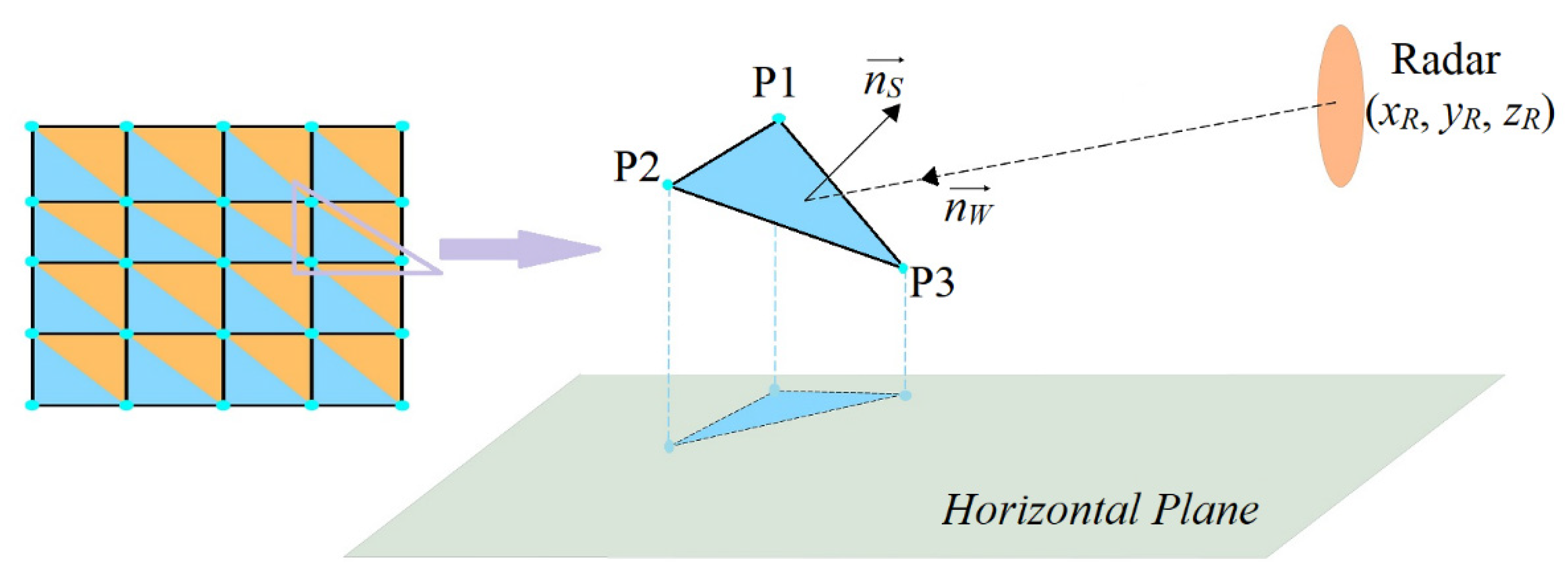
The main part of radar backscattering on the sea surface depends on three factors: beam width, radar antenna height, and beam incidence angle. Assuming that the radar beam is a needle beam, the radar footprint is approximately an ellipse. In practice, the radar signal processor samples the echo within a certain gate. A certain size of the rectangular box is selected such that the rectangular box contains the part of the sea surface both within the gate and in the radar footprint, as shown in Figure 1.

Figure 1.
The schematic division of scattering cells in the radar footprint.
The length of the rectangular box is equal to the radar gate width, i.e., the distance between ymax and ymin in the figure. The width of the rectangular box rw is equal to the length of the short axis of the ellipse formed by the radar footprint, which can be calculated from the grazing angle and the 3 dB beam width:
where θ3dB is the 3 dB beam width, h is the radar height, ymin is the projection of the starting position of distance sampling points on the y-axis, and ymax is the projection of the stopping position of distance sampling points on the y-axis.
The horizontal and vertical segmentation intervals are c/2fs and yminδα.
where Np is the number of pulses in a coherent processing interval (CPI), c represents the speed of light, fs is the pulse sampling frequency, and βσ denotes the pitch angle of the scattering cell relative to the radar.
Every three coordinates of the sampling point on the sea surface can determine a triangular scattering cell. The scattering element has three properties: position, size, and direction. The relationship between one scattering element and radar position is shown in Figure 2.
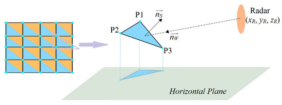
Figure 2.
The relative position of scattering cell and radar.
The three vertex coordinates of the scattering element can be expressed as P1 (x1, y1, z1), P2 (x2, y2, z2), and P3 (x3, y3, z3); then, the center position coordinates of the scattering cell can be calculated as follows:
The normal vector of scattering cell is expressed as:
The area of the scattering cell is:
Defining the radar coordinate as (xR, yR, zR), the incident wave direction can be calculated as:
The local incident angle of the scattering cell can be expressed as:
The azimuth and pitch angle of the scattering cell are:
2.2.4. The Backscattering Coefficient Model
The normalized scattering coefficient is related to several factors that may be difficult to obtain directly through calculations. Numerous empirical models were generated that use large numbers of observations, e.g., RRE, GIT, Sittrop, and TSC. These models can be used to estimate the scattering coefficient of the sea surface with a grazing angle of less than 10 degrees [4,10]. With the development of physical modeling, composite models were developed. The most recognized is the two-scale model, which shows the small-scale Bragg waves being modulated by large-scale gravity waves. The variable slopes of the sea surface at the incident position change the incident angle accordingly so that the backscattering coefficient changes with time and space position. This provides a simple description of the complex sea clutter correlation characteristics [37]:
such that
where ϕ is the local incidence angle, α is the azimuthal angle, kB = 2ksinϕ is the Bragg wave number, ε is a constant related to the medium, and S (k, α) is the surface elevation spectrum. The subscripts VV and HH represent vertical and horizontal polarization modes.
2.2.5. Breaking Wave Model
Under high resolution and low grazing angle, sea spikes are prone to occur in sea clutter. There is no strict physical explanation and mathematical model for the generation of sea spikes so far, but some researchers confirmed that the sea spikes mainly come from the sea surface breaking waves, and the sea spikes generated by different breaking waves are also different [10]. After the wave enters the shallow water area with decreasing depth, the wave steepness gradually increases, and the wave breaks when the steepness reaches the limit [33]. The breaking wave will form a large spike, a major focus of sea clutter research. The maximum wave height of a deep-water wave is limited by the maximum wave steepness in which the waves can remain stable. When the maximum wave steepness is reached, the waves will break. Stokes pointed out that the wave steepness limit is achieved when the horizontal trajectory velocity of the water particle on the wave crest is exactly equal to the wave velocity. At this time, the wave crest is steep and unstable, and the wave crest angle is equal to 120° [38] (see Figure 3).
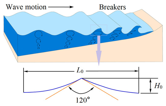
Figure 3.
Limit wave steepness and crest angle in deep water.
Based on the limit crest angle, Michell [39] proposed that the wave steepness limit for deep-water propulsion waves is:
where H denotes wave height, L denotes wavelength, and subscript 0 denotes deep water.
When the wave enters the shallow water area, the ultimate wave steepness is not a constant and is related to the relative water depth. Miche [40] recommends that the limiting wave steepness under limited water depths and horizontal bottom slopes be determined by the following formula:
where k (consistent with earlier) indicates the wave number and h denotes water depth. In shallow water, where , the wave steepness limit can be expressed as:
Note that the nonlinear parameter δ calculated based on the wind speed in the previous paper is equivalent to the average wave steepness of the entire simulated sea surface. In order to use the limit wave steepness as the threshold to determine whether a breaking wave occurs, it is necessary to infer the wave steepness distribution of the simulated sea surface according to the known average wave steepness. Given that the wave steepness obeys the Rayleigh distribution [41], the Rayleigh distribution function with an average value of δ is:
The proportion of x > 0.142 is calculated as 1 − exp (−0.016/δ2). Assuming that the wavelength of the simulated sea surface is similar, the wave steepness is proportional to the wave height. In this case, the ratio of wave steepness, which is larger than 0.142, can be used as the threshold of the breaking wave height. The large wave heights in the wave height field are determined using this ratio, and their plane coordinates are marked to determine the location of the breaking wave.
The RCS of breaking waves [42] can be expressed as:
where is the RCS of breaking waves, is the grazing angle, is the wave number of radar electromagnetic, and °. The spectrum of the Bragg waves is denoted by , i.e., , and the breaking wavelength can be expressed as .
2.3. Workflow of Sea Clutter Signal Model
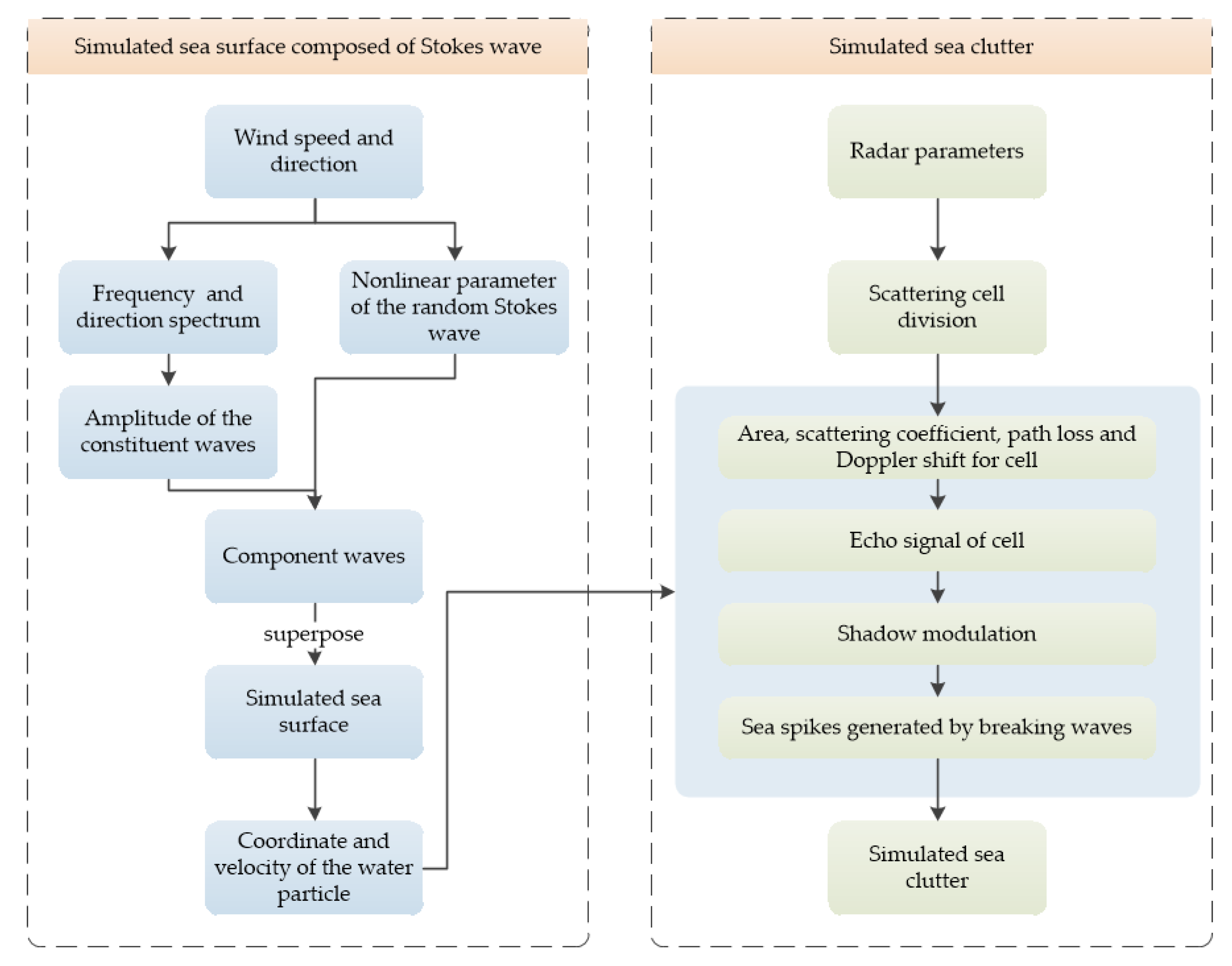
The sea clutter signal simulation scheme in this paper is divided into two parts: sea surface simulation and sea clutter simulation. In Section 2.2, the realization method of each module in each part is introduced in detail. This part will show the implementation steps of the overall scheme in the form of a workflow diagram (see Figure 4).

Figure 4.
Workflow of the sea clutter signal model.
In the sea surface simulation part, first, the sea condition parameters, i.e., the wind speed and direction, need to be set. Then, the component wave amplitude and the nonlinear parameter of the Stokes wave are calculated, which determine the waveform of the component wave. The superimposed component wave constitutes the simulated sea surface, and the coordinate of each node represents the position of the water quality point. The velocity of the water quality point is obtained by the derivation of the position.
In the sea clutter simulation part, the working parameters of the radar should be set to determine the radar transmit signal. When calculating the area, scattering coefficient, path loss, and Doppler frequency shift of each scattering cell, it is necessary to use the position and velocity of each water quality point in the simulated sea surface. The shadow modulation and breaking wave deployment also depend on the relative positions of water points.
3. Results
3.1. Simulations Results
A 30 s simulation test was performed in this study. The environmental parameters and radar parameters are listed in Table 1.

Table 1.
Simulation parameters.
In the experiment, a set of the simulated sea surfaces was first generated by setting the wind speed to 10 km/h and 20 km/h, and the wind direction, which approximates wave direction, was set to 300 degrees. The minimum wind speed in the P–M spectrum is 3.46 m/s, i.e., 12.46 km/h [35]. The P–M spectrum is an empirical spectrum obtained by data fitting, and the boundary value should be an approximation, so it is set to 10 km/h to simulate the sea surface under a low sea state. The wind speed of 20 km/h corresponds to Douglas sea state level 2, which is one of the most common sea states in reality. Therefore, the wind speed is set to 20 km/h to simulate the sea surface under a normal sea state.
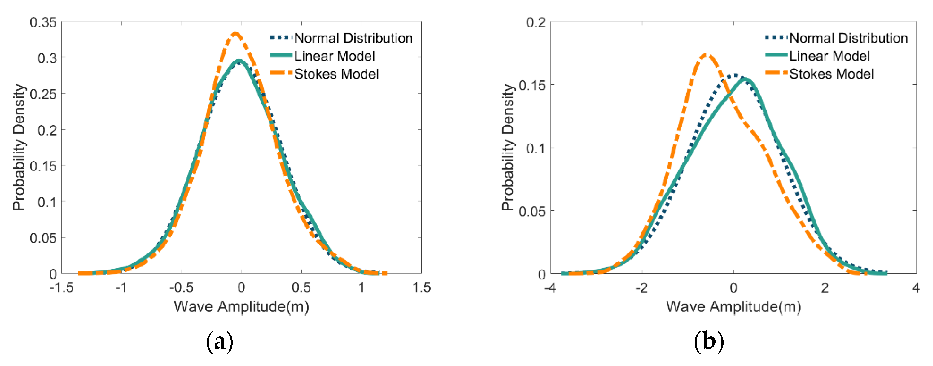
The linear wave superposition model and the Stokes wave superposition model were used to simulate the same scenarios, and the nonlinear characteristics of the simulated sea surface were tested using the statistical distribution of the wave heights. As shown in Figure 5, the wave height of the linear wave model follows a normal distribution, while the wave height of the Stokes wave model follows a skewed distribution. The simulations show that the higher the wind speed, the greater the deviations from the normal distribution. This finding is consistent with the theory that wind speed is proportional to wave steepness.

Figure 5.
Comparison of the wave height distribution with normal distribution between the linear model and the Stokes model under different wind speeds: (a) wind speed at 10 km/h, (b) wind speed at 20 km/h.
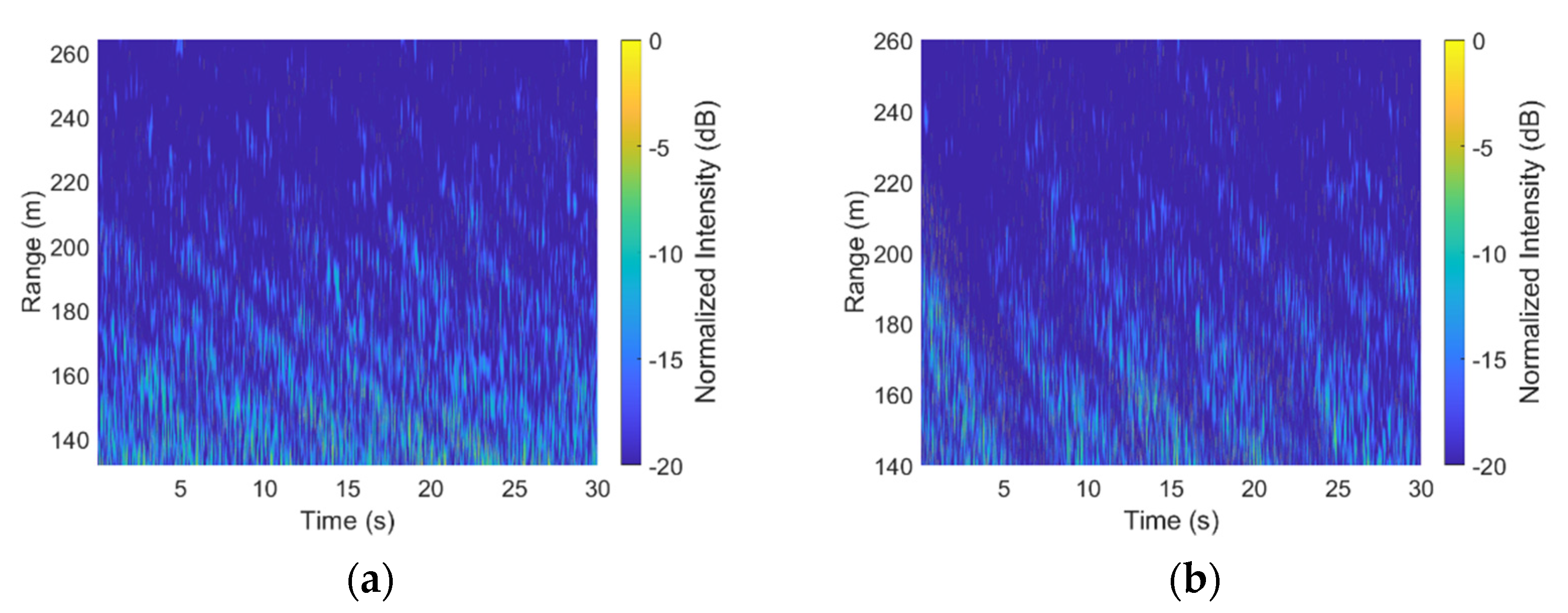
After obtaining the wave height field from the simulation, the scattering intensity was calculated, and the shadow modulation was performed. In addition to the effects of noise, path loss, and phase jitter, the simulated sea clutter was generated. Figure 6 shows the simulated sea clutter intensity in the range of partial radar line of sight. The intensity plots exhibit periodicity in the distance dimension, and the higher the set wind speed, the longer the period. In addition, the lower the wind speed, the more scattered spots in the intensity map, since the simulated waves at low wind speeds are more finely divided, corresponding to more scattered backward scattering.
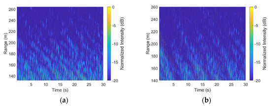
Figure 6.
A part of the simulated sea clutter intensity map under different wind speeds: (a) wind speed at 10 km/h, (b) wind speed at 20 km/h.
3.2. Comparison with Simulations and Actual Measurements
In November 1993, a large database of high-resolution radar measurements was collected using the McMaster IPIX radar at the east coast of Canada from a clifftop near Dartmouth, Nova Scotia (44°36.72′N; 63°25.41′W), on a cliff facing the Atlantic Ocean, 100 feet above mean sea level with an open ocean view of about 130°. The 339 data sets in the database cover a wide range of conditions: wave conditions: 0.8–3.8 m (peak height up to 5.5 m) and wind conditions: 0–60 km/h (gusts up to 90 km/h). The 0 degree in the wind direction indicates the positive north direction.
The IPIX radars were all working at 9.39 GHz at the time of acquisition, irradiating a fixed orientation for about 2 min in the dwell mode with a low grazing angle, a pulse repetition frequency (PRF) of 1000 Hz, and a distance sampling interval of 15 m. The cooperative target on the sea surface is a spherical foam wrapped with steel wire with a diameter of about 1 m. Under this measurement condition, each data file obtained contains 4 sets of echo data with different polarization modes, each containing a continuous complex signal sequence of 14 range bins with a sequence length of 217 (corresponding to an observation time of 131.72 s). The IPIX data are open data commonly used in sea clutter research.
To quantitatively analyze the simulated sea clutter, the estimates were compared with real measured clutter data, part of the IPIX 1993 dataset (see Table 2). The wind speed (U) and wind direction (Wd) corresponding to each actual measurement were acquired from the official website. A set of real measured data with the same wind direction and different wind speeds was used for the subsequent experiments.

Table 2.
IPIX data.
3.2.1. Comparisons of Clutter Intensity
IPIX #54 was chosen for the comparative analysis since its wind speed is at mid-value and is a common wind speed in real sea conditions. Figure 7a presents the variations in the range–pulse dimension simulated signal intensity when the wind speed is set to 19 km/h. Based on the figure, there is a periodic variation in the intensity of different pulse signals in the same range bin. The intensity between various distance sampling points of the same pulse decreases with increasing distance. In addition, the figure shows directivity, which is consistent with the wave direction (300°) angle set by the simulation. Figure 7b shows the intensity of #54 IPIX data.
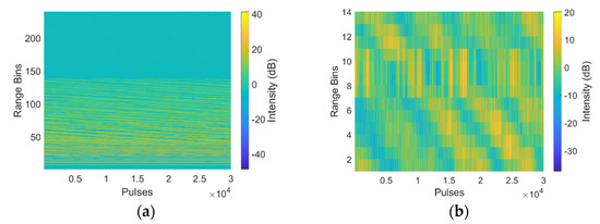
Figure 7.
Sea clutter intensity map: (a) simulated intensity map; (b) #54 IPIX data intensity map.
Comparing (a) and (b) in Figure 7, the simulated sea clutter wave shown in (a) is continuous in intensity and uniform in slope, while the real measured sea clutter wave shown in (b) has a strong echo at the position of range bins 7 to 11 that is not coherent with other parts. The #54 real measured sea clutter wave has a target placed at the position of range bin 8, and several surrounding bins are affected by the target. In the subsequent comparison experiments, the pure sea clutter data from the real measured data were chosen as the comparison data, and the influence of the target on the sea clutter properties was removed.
In addition, the echo intensity demonstrated in Figure 7a shows a uniform weakening as the range bin increases from small, while Figure 7b shows no significant intensity change in the distance dimension. The simulated scenario contains more than 200 range bins, corresponding to a distance range of 2 km, while the real measured sea clutter wave has only 14 range bins, which is too small a distance range and does not reflect the intensity variation pattern in the distance.
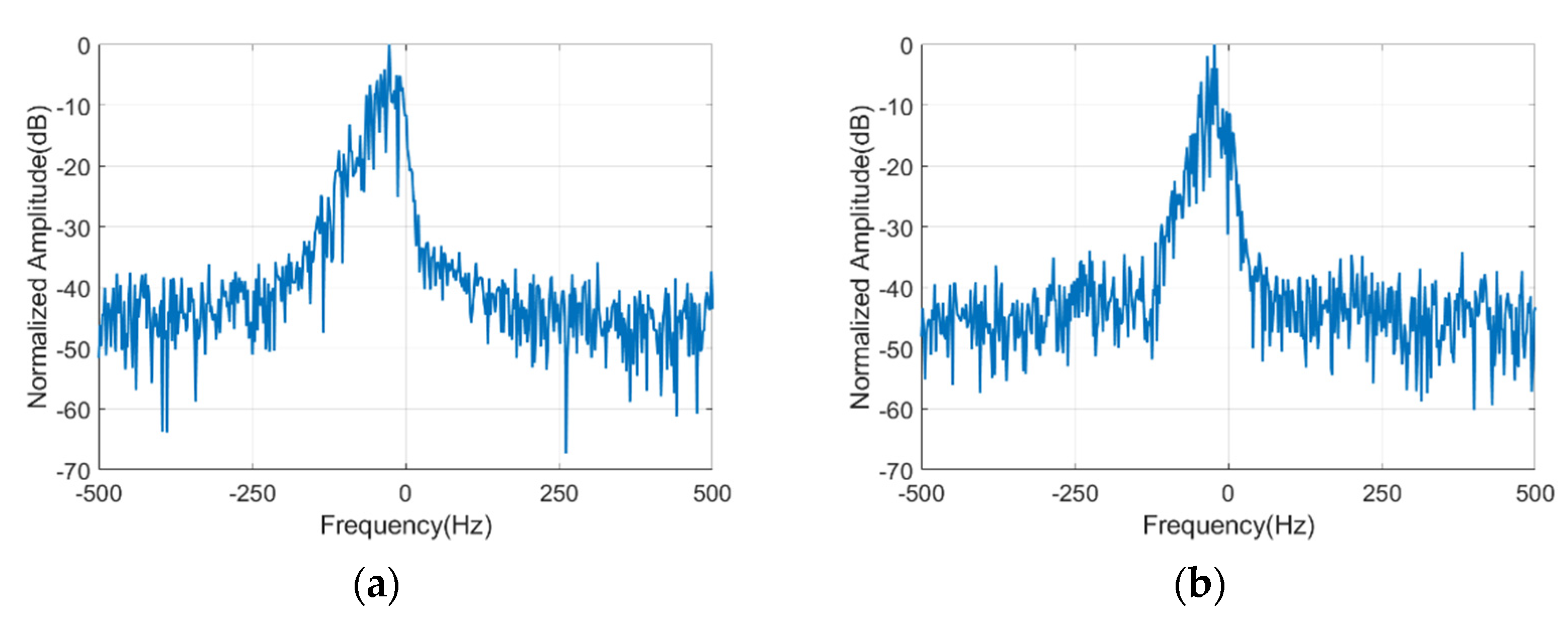
The intensity map shows periodicity in the distance direction and can be visualized using the intensity from a single pulse. As shown in Figure 8, the simulated and real measured intensity values have similar repetition periods. The surface fluctuates with the motion period because of the approximate circular motion made by the water particles at the corresponding positions. Therefore, the periodic variation in the backscattering cross-section leads to the systematic variation in echo intensity. The period of intensity change is consistent with the period corresponding to the peak of the P–M spectrum, which is the main wave period. Here, the period is about 8.5 s.
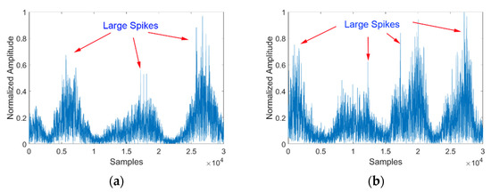
Figure 8.
The intensity of sea clutter from a single range bin: (a) simulated data; (b) #54 IPIX data.
On the other hand, as presented in Figure 8a, multiple spikes are generated in the echo due to the addition of breaking waves in the model. The spike intensity is comparable with the real measured sea clutter values in Figure 8b. This suggests that the model can simulate the white-crown scattering phenomenon of sea clutter.
3.2.2. Comparisons of Amplitude Statistics
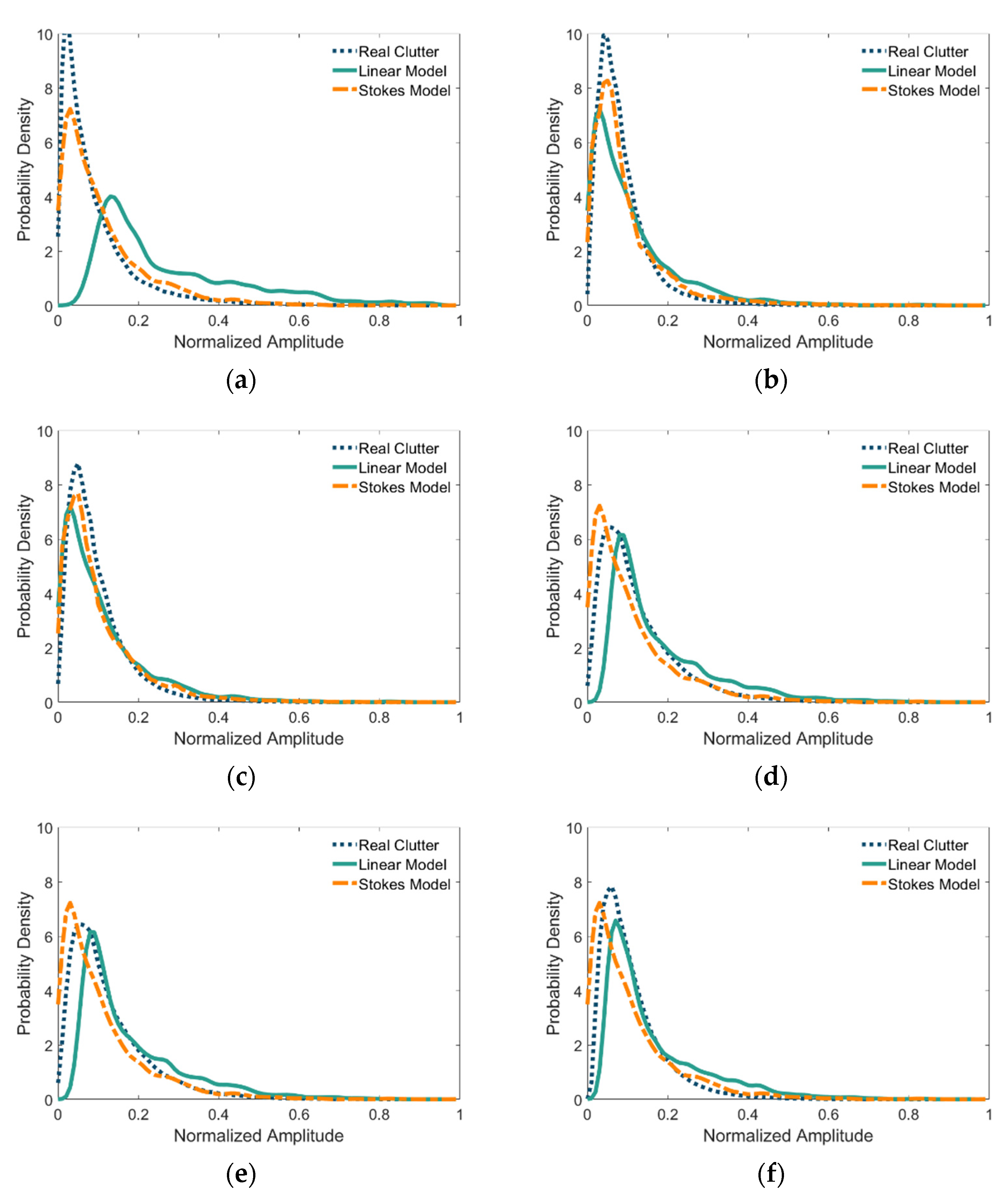
The amplitude statistical characteristics of the simulated sea clutter were then analyzed. The two sea clutter types were simulated using the linear model and the Stokes model, and the simulation results were compared with actual sea clutter measurements. Figure 9 shows the comparison results of six groups of different wind speeds. Compared with the amplitude distribution of the linear model, the distribution curve of the Stokes model fits better with the real measured clutter at the tail.
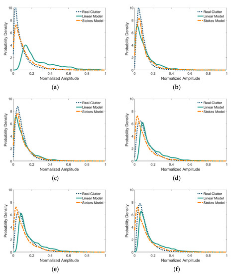
Figure 9.
Comparison of the normalized amplitude probability distribution of real measured sea clutter and simulated clutter: (a) #17 IPIX data and simulations; (b) #31 IPIX data and simulations; (c) #40 IPIX data and simulations; (d) #54 IPIX data and simulations; (e) #310 IPIX data and simulations; (f) #320 IPIX data and simulations.
The goodness of fit can reflect the degree of fitting between the amplitude statistical model and actual measurements. The Rayleigh, lognormal, Weibull, and K tests were selected for the amplitude statistical model, while the chi-square test, Kolmogorov–Smirnov (K–S) test, and mean square difference (MSD) were used in the evaluation. Using the same simulation parameters as the #54 data, 50 Monte Carlo experiments were performed, and the mean coefficient of determination was calculated. Table 3 presents the fit results of the simulation data. The experimental results show that the simulated sea clutter amplitude distribution is closer to the K-distribution. It was demonstrated that the K-distribution has good results in describing the sea clutter amplitude statistics compared with common statistical distribution models such as Rayleigh and Weibull [10].

Table 3.
Results of the goodness-of-fit test.
3.2.3. Comparisons of Doppler Spectrum Features
In addition to amplitude statistics, the Doppler spectrum is another key feature of sea clutter. Here, the simulated sea clutter was generated based on the parameters of #54. Taking this data point as an example, the simulated sea clutter and the real measured clutter were compared and analyzed.
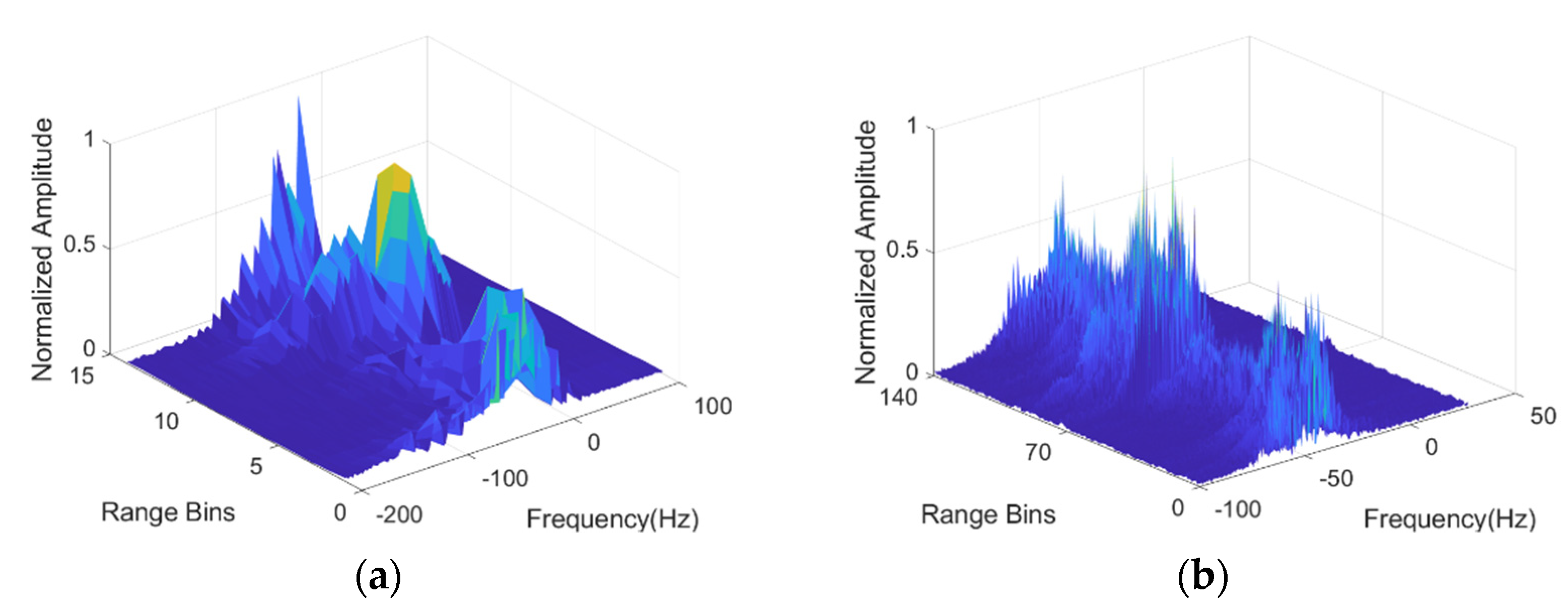
The pulse-dimensional fast Fourier transform (FFT) was performed on the range–pulse signal, and the Doppler spectrum of multiple range bins was obtained. Figure 10 shows the range–Doppler spectrum of simulated clutter and real measured clutter. Given that there are other objects in the real measured data, the middle position shape of the Doppler spectrum is inconsistent with the head and tail. The real measured sea clutters mentioned in this paper are pure sea clutter data after removing the outliers.
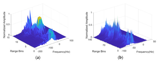
Figure 10.
Range-Doppler spectrum of sea clutter: (a) spectrum of real measured clutter; (b) spectrum of simulated clutter.
In Figure 10a,b, the frequencies corresponding to the positions of the spectral peaks indicate the Doppler frequency shift of the sea clutter waves, and the spectral broadening phenomenon indicates that there are multiple velocity components in the waves. The Doppler spectral peak in (b) appears at −50 Hz, indicating that the overall surface velocity of the wave is 0.8 m/s. In (a), on the other hand, strong energy appears beyond −50 Hz because of the target in bin 8.
The range-Doppler spectrum deviates from the zero frequency, indicating that the sea clutter has a certain velocity. However, the range-Doppler spectrum is not fixed in the direction of the range bin. Both the spectral peak and the spectral width fluctuate with a change in the range, indicating that the motion characteristics at different range bins are not completely consistent. Therefore, the Doppler spectrum characteristics have to be analyzed from multiple perspectives.
First, the spectrum is analyzed from the frequency dimension, and the range-averaged Doppler spectrum is obtained by taking the average for all range bins. As shown in Figure 11, the simulated spectrum and the real measured spectrum have similar spectral peaks and widths. Their spectrum shapes are comparable, which indicates that without considering the distance factor, the simulated sea clutter has a similar overall velocity to actual measurements and has multiple frequency components that can effectively reflect the motion characteristics of the real sea clutter.
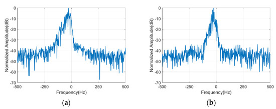
Figure 11.
Range-averaged Doppler spectrum of sea clutter: (a) spectrum of real measured clutter; (b) spectrum of simulated clutter.
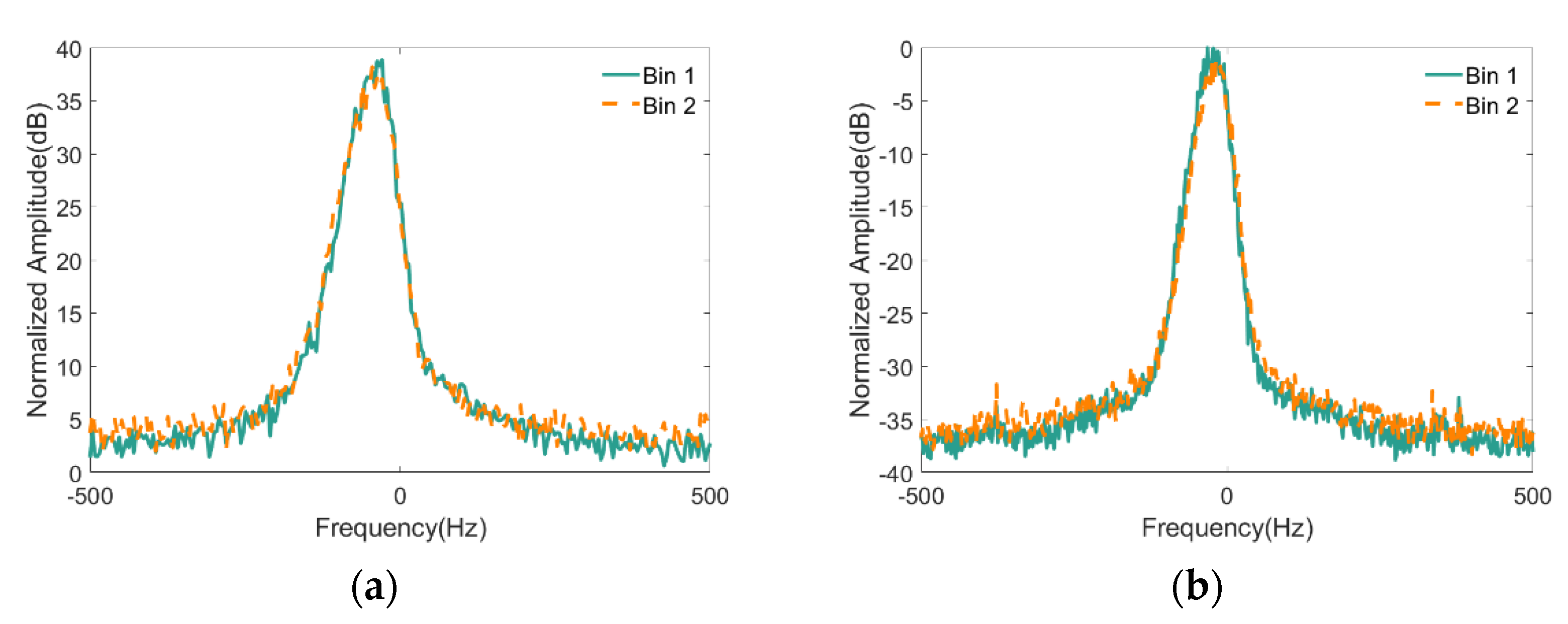
Figure 12 shows the Doppler spectra from a single range bin obtained using Fourier transform. While the Doppler spectral peaks of real measured from different range bins are similar, the spectral widths and bottom noise are different. The simulated sea clutter can reproduce the spectral peak characteristics, but the spectral width and the bottom noise are not significantly divergent with different range bins.
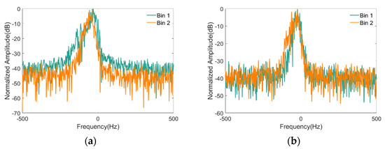
Figure 12.
Doppler spectrum from a single range bin: (a) spectrum of real measured clutter; (b) spectrum of simulated clutter.
The average Doppler spectrum from a single range bin was then analyzed. The same range bin data from Figure 12 were selected and divided into multiple segments based on the PRF length. For each segment, a 512-point FFT was employed, and the average values on all segments were calculated to obtain the mean Doppler spectrum. The results are shown in Figure 13.
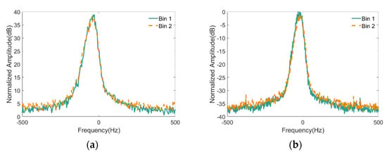
Figure 13.
Average Doppler spectrum from a single range bin: (a) spectrum of real measured clutter; (b) spectrum of simulated clutter.
The real measured sea clutter Doppler spectrum from different range bins has no significant difference, and the average Doppler spectrum of simulated sea clutter can adequately characterize the actual spectrum. This also explains that the traditional method of simulating the average Doppler spectrum of sea clutter with the Gaussian spectrum is effective because of the consistency of the average Doppler spectrum.
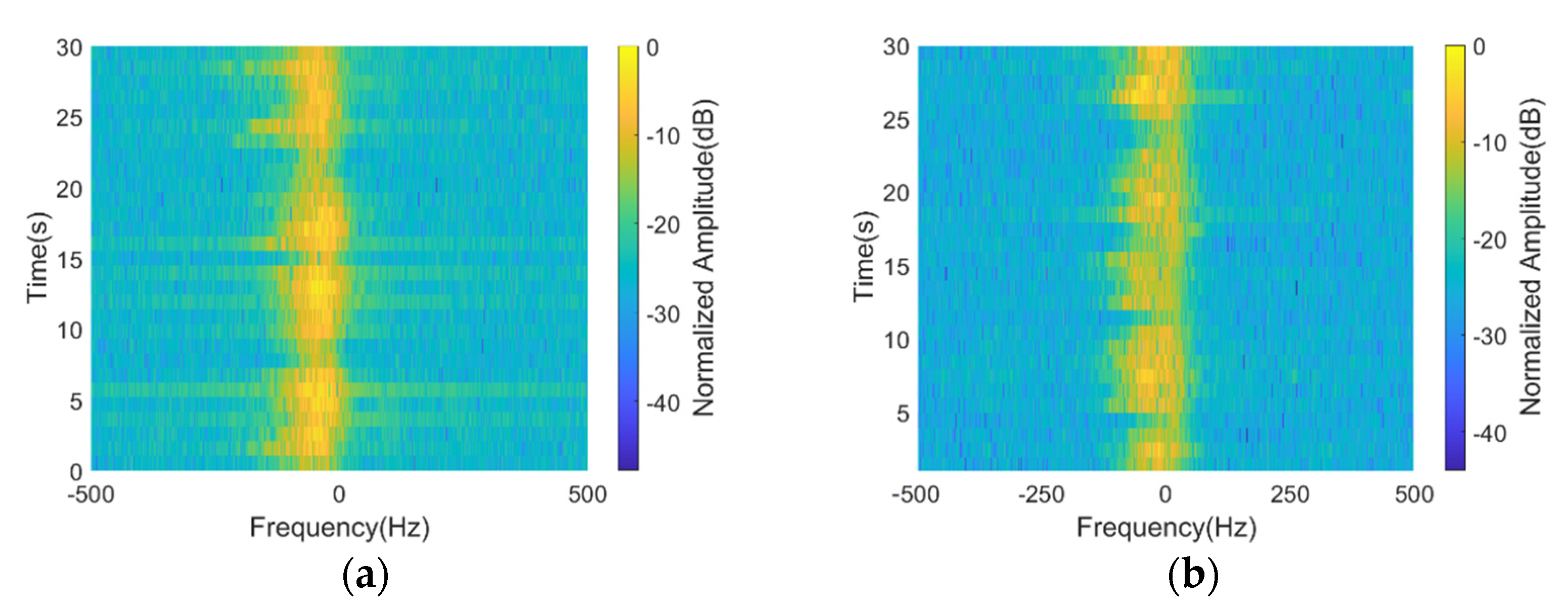
Another important feature of the sea clutter Doppler spectrum is its time-varying characteristics. Even the Doppler spectrum of the same range bin will fluctuate over time. For this study, the sea clutter from a single range bin was divided into 30 time segments, forming a 1000 × 30 data matrix. The 128-point FFT was performed in the direction of the matrix column, and the results are shown in Figure 14a. The spectra of the real measured sea clutter have pronounced intensity modulation, and their shapes changed and showed offset. Due to the combined effect of the surge and the local wind, the maximum Doppler frequencies at different times had noticeable changes in the time dimension and a temporal periodicity similar to the intensity map can be seen. The simulation data at identical distances were selected to calculate their time-varying Doppler spectra, as shown in Figure 14b. The results indicate that the simulated spectra also have intensity modulation and periodic variation. Since the proposed model is based on the scattering mechanism of the dynamic sea surface, it has time-varying characteristics similar to actual sea clutter measurements.
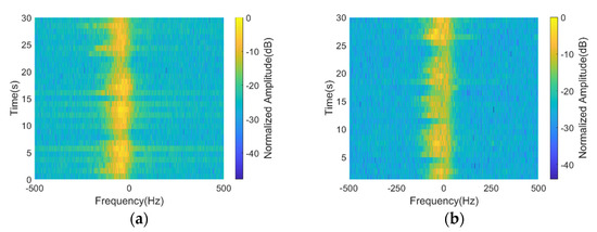
Figure 14.
Time history of sea clutter Doppler spectra from a single range bin: (a) spectra of real measured clutter; (b) spectra of simulated clutter.
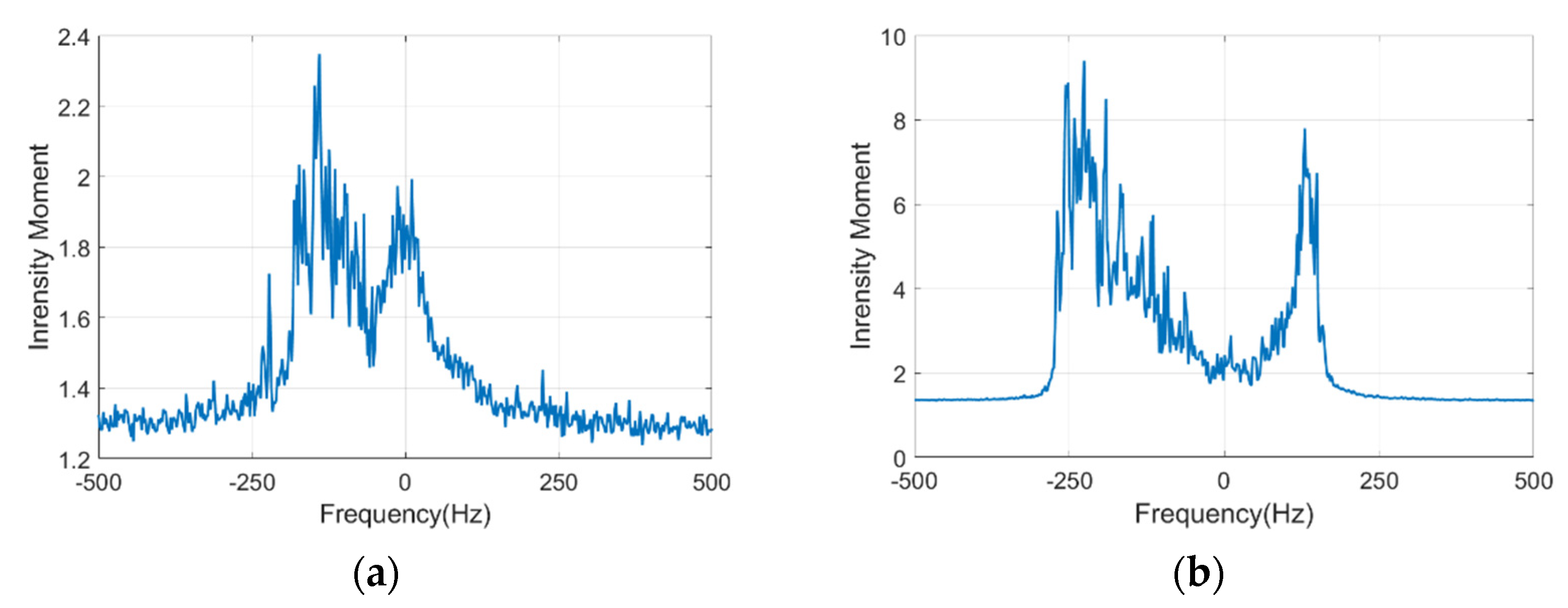
Numerous studies were conducted to explore the non-Gaussian characteristics of the sea clutter spectrum, often employing the standardized second-order intensity moment. For Gaussian clutter (or noise), the value of the standardized second-order intensity moment is 2, which can be used as the threshold to determine whether the clutter has a non-Gaussian character. The sharper the clutter, the larger the corresponding value.
As shown in Figure 15a, the standardized second-order moment of actual sea clutter measurements is larger where the echo intensity is significant. Figure 15b shows the plot of the standardized second-order intensity moment of the simulated sea clutter. Similar to actual measured data, the peak appears on both sides of the zero frequency; the maximum deviates from the zero frequency and is greater than 2.
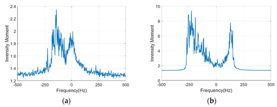
Figure 15.
Standardized second-order intensity moment of the Doppler spectrum: (a) real measured clutter; (b) simulated clutter.
The plotted results also show considerable differences. The intensity moment is greater than the actual sea clutter measurement, the peak interval on both sides of zero frequency is significantly greater than the real measured data, and the edge transition is more rapid. These differences suggest that the boundary between clutter and noise in simulated sea clutter is pronounced and that the clutter at near-zero frequency is submerged by noise. This proves that even though the nonlinear actual wave waveform and complex process of electromagnetic scattering are fully considered in the model, gaps remain between the simulated clutter and the actual clutter.
To analyze the spectral peaks and spectral widths of sea clutter Doppler spectra for different wind speeds, comparative simulation tests were conducted, ensuring that all their parameters remained consistent and that only the wind speeds were changed. The wind speed varied in 0.5 steps in the 10–40 km/h range. The Doppler spectrum was estimated by the third-order autoregressive (AR) spectrum.
In this paper, the spectral peak and spectral width were used to characterize the Doppler spectral characteristics. The spectral peak is the frequency corresponding to the spectral maximum, and the spectral width pertains to the width at the amplitude decrease of 20 dB. The estimation results for the six sets of IPIX data Doppler spectra information are summarized in Table 4.

Table 4.
IPIX data Doppler spectra.
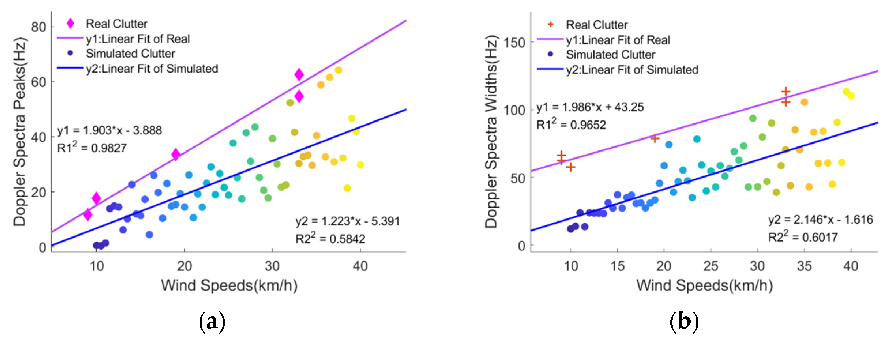
Figure 16 shows the results of spectral estimation. The diamond and cross represent the real measured values, and the circular scatters correspond to the simulated values. As presented in the figure, the Doppler spectral peaks and widths of the simulated clutter values are generally close to the actual measurements. The peaks and widths are proportional to wind speed.
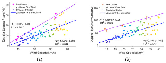
Figure 16.
Characteristics of the Doppler spectra under different wind speeds (the wind speeds change from 10 km/h to 40 km/h in steps of 0.5): (a) peaks of Doppler spectra; (b) widths of Doppler spectra.
The simulated spectral peaks and widths are slightly smaller than the real measured values, and the estimates are unstable at higher wind speeds. The Doppler spectra widths of simulated clutter differ from those of actual clutter measurements, especially at low wind speeds. This phenomenon may be caused by ignoring the effect of surface velocity on dispersion relation in this model. The large fluctuation of spectral peaks and widths may be due to the bimodal nature of the model.
The linear fitting results for the actual and simulated clutter data are shown in Figure 16. The * in the linear fit equation indicates the multiplication sign. The correlation coefficient of real measured data is above 0.9, while that for the simulated data is only about 0.6. However, it is uncertain whether the fitting difference is widespread because of the inadequacy of real measured samples.
3.2.4. Comparisons of Related Features
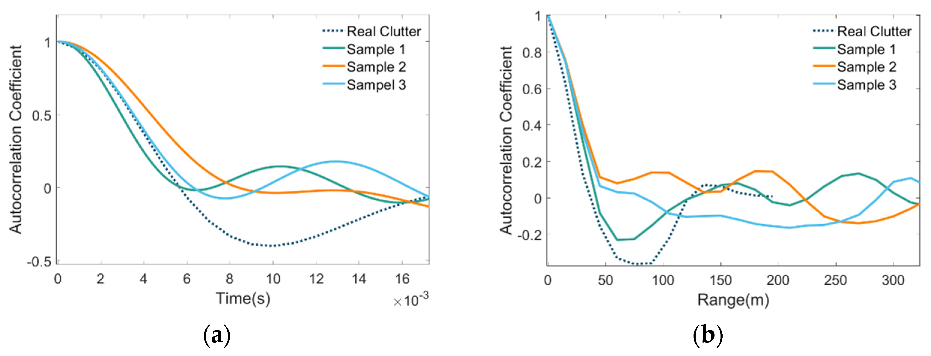
For a dynamic sea clutter model, in addition to checking its amplitude statistical distribution and Doppler characteristics, its correlation properties also need to be tested. The correlation properties of sea clutter include temporal and spatial correlations, generally described by the autocorrelation coefficient. Figure 17a shows the temporal autocorrelation correlation curve, and Figure 17b shows the spatial autocorrelation correlation curve. As shown in the figures, the autocorrelation coefficients of temporal samples decrease to 0 after about 6 milliseconds, and the autocorrelation coefficients of spatial samples decrease to 0 after about 50 m. Although there are differences among samples, the simulated estimates are generally comparable with real sea cluster measurements in terms of temporal and spatial correlations.
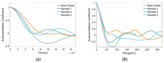
Figure 17.
Comparison of the autocorrelation correlations between different simulated samples and the real measured sea clutter: (a) temporal autocorrelation correlations; (b) spatial autocorrelation correlations.
4. Discussion
When the location of the large spikes was further analyzed, the simulation spikes were largely found distributed in the peak position of the sea clutter intensity envelope (see Figure 8a). This phenomenon is related to the way that the breaking wave positions are determined by wave steepness. The higher the wave, the greater the wave steepness and the greater the probability of being evaluated as a breaking wave. Although the shadow effect is processed later, the breaking wave is generally distributed around the large wave height. The strong scattering in the simulated sea clutter corresponds to the large wave height, so the spikes are concentrated around the wave crest. However, the position of the white crown on the actual sea surface is not always distributed near the large wave height (see Figure 8b). Due to the influence of wavelength, even if the wave height is small, a breaking wave may still be formed, causing the peak position of the actual sea clutter to be more dispersed.
Compared with the linear model, the amplitude distribution curve of the Stokes model fits better with the real measured clutter. The large wave height distribution of the linear model is relatively uniform, and the corresponding strong echo distribution changes will be relatively flat. Similar to the actual shape of ocean waves, the Stokes waveform peak is sharp, and the trough is flat, which means that the corresponding sea clutter is closer to the real measured value. On the other hand, at low wind speeds, the uniformity of linear superposition waves is more pronounced, causing the amplitude distribution of the linear simulations and the actual clutter measurements to differ slightly. The Stokes model uses the nonlinear characteristics of the waveform, thus significantly improving the estimation results, as shown in Figure 9a.
The ordinary waveform model assumes that the water particle moves circularly, but in reality, water particles have unclosed elliptical trajectories. Therefore, the Stokes wave model proposed in this paper is closer to the actual wave. In addition to the waveform function, the statistical distribution of simulated wave height can also confirm this point (see Figure 5). However, the Doppler velocity of the actual sea clutter is a composite result formed by the tangential velocity of elliptical motion and the overall moving velocity of the sea surface. This results in the Doppler spectral peak and width of the simulated clutter being less than the actual measurement. Introducing the dispersion relationship with surface velocity in the model may solve this problem, but the surface velocity needs to be transformed in the electromagnetic scattering calculation.
Different wave spectrum types may also affect the simulation results. The P–M spectrum in this model can be replaced by other spectrum types to simulate sea clutter in specific scenarios.
The detailed modeling of breaking waves is also more complex than the proposed method and requires the consideration of the number of breaking waves and their shapes. In studies on the impact of the breaking wave, appropriate fluid mechanics methods can be used to accurately model the breaking wave. However, this greatly increases computational complexity, which may not be suitable for real-time simulation situations.
In terms of transmission path loss, the ideal atmospheric loss model may not be able to fully conform to the actual conditions. In cases of low incident angle, most electromagnetic waves are transmitted in the steam waveguide of the sea surface so that the path loss can be added to the influence of the transmission medium.
Note that in this paper, the actual and the simulated sea clutter are both vertical transmit and vertical receive (VV) polarization data. The influence of different polarization modes on the simulations is beyond the scope of this paper, so there was no comparative analysis of the various polarization models. However, apart from the experiments in this paper, horizontally polarized sea clutters were simulated to verify that the proposed method can still be effective after changing the polarization mode.
5. Conclusions
This study developed a sea clutter simulation scheme for shore-based radar systems, which typically have large incidence angles, significant nonlinearity of wave forces, and frequent breaking wave actions. The random Stokes wave was used as the component wave in the dynamic sea surface model, and the simulated sea clutter was generated through electromagnetic wave irradiation on the sea surface. In the proposed method, the breaking wave model, shadow effect, and scattering cell division were also considered to restore the sea clutter generation process from the perspective of electromagnetic wave transmission.
Using the relationship between wind speed and wave nonlinearity, the proposed approach establishes the link between wave nonlinearity and the number of breaking waves. The developed model enhances the dynamic influence of the sea state on clutter based on existing models. The simulations show that the simulated clutter is consistent with actual clutter measurements in intensity, amplitude distribution, Doppler spectrum, and spatial-temporal correlation. Accordingly, this scheme can be adopted as an original approach for dynamic sea clutter simulation.
The research provides an innovative strategy for sea clutter simulation in littoral waters. The breaking waves, shallow waters, rocks, and offshore winds can be regarded as additional models in sea surface simulation. These factors make sea clutter in littoral waters extremely complex, directly affecting the shape of the sea surface. Aside from the electromagnetic scattering model, significant consideration should be given to the irradiated sea surface, the physical relationship between the radar and the sea surface, and the transmission process of electromagnetic waves.
Author Contributions
Y.F. designed the simulation model and wrote the manuscript. F.L. supervised the preparation of the manuscript and coordinated revisions. G.L. and L.Z. provided key guidance in this article. All authors have read and agreed to the published version of the manuscript.
Funding
This work was supported in part by the National Key Foundation for Exploring Scientific Instrument (2013YQ20060705).
Data Availability Statement
Not applicable.
Acknowledgments
Thanks to http://soma.ece.mcmaster.ca/ipix/ (accessed on 3 July 2022) site for the IPIX radar data; this site provides the real measured sea clutter data for this research.
Conflicts of Interest
The authors declare no conflict of interest.
References
- Wright, J. A new model for sea clutter. IEEE Trans. Antennas Propag. 1968, 10, 217–223. [Google Scholar] [CrossRef]
- Plant, W.J.; Keller, W.C. Evidence of Bragg scattering in microwave Doppler spectra of sea return. J. Geophys. Res. 1990, 95, 16299–16310. [Google Scholar] [CrossRef]
- Elfouhaily, T.; Chapron, B.; Katsaros, K.; Vandemark, D. A unified directional spectrum for long and short wind-driven waves. J. Geophys. Res. 1997, 102, 15781–15796. [Google Scholar] [CrossRef]
- Karimian, A.; Yardim, C.; Gerstoft, P.; Hodgkiss, W.S.; Barrios, A.E. Multiple Grazing Angle Sea Clutter Modeling. IEEE T. Antenn. Propag. 2012, 60, 4408–4417. [Google Scholar] [CrossRef]
- Horst, M.M.; Dyer, F.B.; Tuley, M.T. Radar sea clutter model. In Proceedings of the IEEE International Conference of Antennas and Propagation, London, UK, 28–30 November 1978. [Google Scholar]
- Ward, K.D.; Watts, S. Use of sea clutter models in radar design and development. IET Radar Sonar Nav. 2010, 4, 146–157. [Google Scholar] [CrossRef]
- Alpers, W.R.; Ross, D.B.; Rufenach, C.L. On the detectability of ocean surface waves by real and synthetic aperture radar. J. Geophys. Res. 1981, 86, 6481–6498. [Google Scholar] [CrossRef]
- Romeiser, R.; Alpers, W.; Wismann, V. An improved composite surface model for the radar backscattering cross section of the ocean surface: 1. Theory of the model and optimization/validation by scatterometer data. J. Geophys. Res. 1997, 102, 25237–25250. [Google Scholar] [CrossRef]
- Jakeman, E.; Pusey, P. A model for non-Rayleigh sea echo. IEEE T. Antenn. Propag. 1976, 24, 806–814. [Google Scholar] [CrossRef]
- Ward, K.D.; Watts, S.; Tough, R.J. Sea Clutter: Scattering, the K Distribution and Radar Performance, 2nd ed.; IET: London, UK, 2013. [Google Scholar]
- Rosenberg, L.; Crisp, D.J.; Stacy, N.J. Analysis of the KK-distribution with medium grazing angle sea-clutter. IET Radar Sonar Nav. 2010, 4, 209–222. [Google Scholar] [CrossRef]
- Farshchian, M.; Posner, F.L. The Pareto distribution for low grazing angle and high resolution X-band sea clutter. In Proceedings of the IEEE Radar Conference, Arlington, VA, USA, 10–14 May 2010. [Google Scholar]
- Al-Ashwal, W.A.; Woodbridge, K.; Griffiths, H.D. Analysis of bistatic sea clutter—Part II: Amplitude statistics. IEEE T. Aero. Elec. Sys. 2014, 50, 1293–1303. [Google Scholar] [CrossRef]
- Ward, K.D. Compound representation of high resolution sea clutter. Electron. Lett. 1981, 17, 561–563. [Google Scholar] [CrossRef]
- Rangaswamy, M.; Weiner, D.; Ozturk, A. Computer generation of correlated non-Gaussian radar clutter. IEEE T. Aero. Elec. Sys. 1995, 31, 106–116. [Google Scholar] [CrossRef]
- Marier, L.J. Correlated K-distributed clutter generation for radar detection and track. IEEE T. Aero. Elec. Sys. 1995, 31, 568–580. [Google Scholar] [CrossRef]
- Walker, D. Experimentally Motivated Model for Low Grazing Angle Radar Doppler Spectra of the Sea Surface. IET Radar Sonar Nav. 2000, 147, 114–120. [Google Scholar] [CrossRef]
- Davidson, G. Simulation of coherent sea clutter. IET Radar Sonar Nav. 2010, 4, 168–177. [Google Scholar] [CrossRef]
- Watts, S. Modeling and Simulation of Coherent Sea Clutter. IEEE T. Aero. Elec. Sys. 2012, 48, 3303–3317. [Google Scholar] [CrossRef]
- Watts, S.; Rosenberg, L.; Bocquet, S.; Ritchie, M. Doppler spectra of medium grazing angle sea clutter; Part 1: Characterisation. IET Radar Sonar Nav. 2016, 10, 24–31. [Google Scholar] [CrossRef]
- McDonald, M.; Cerutti-Maori, D. Multi-phase centre coherent radar sea clutter modelling and simulation. IET Radar Sonar Nav. 2017, 11, 1359–1366. [Google Scholar] [CrossRef]
- Bocquet, S. Compound G2 model of coherent radar sea clutter. IET Radar Sonar Nav. 2019, 13, 1508–1518. [Google Scholar] [CrossRef]
- Watts, S.; Rosenberg, L. Challenges in radar sea clutter modelling. IET Radar Sonar Nav. 2022, 16, 1403–1414. [Google Scholar] [CrossRef]
- Xin, Z.; Liao, G.; Yang, Z.; Zhang, Y.; Dang, H. A Deterministic Sea-Clutter Space–Time Model Based on Physical Sea Surface. IEEE T. Geosci. Remote. 2016, 54, 6659–6673. [Google Scholar] [CrossRef]
- Huang, P.; Zou, Z.; Xia, X.; Liu, X.; Liao, G.; Xin, Z. Multichannel Sea Clutter Modeling for Spaceborne Early Warning Radar and Clutter Suppression Performance Analysis. IEEE T. Geosci. Remote Sens. 2021, 59, 8349–8366. [Google Scholar] [CrossRef]
- Bai, W.; Eatock Taylor, R. Fully nonlinear simulation of wave interaction with fixed and floating flared structures. Ocean Eng. 2009, 36, 223–236. [Google Scholar] [CrossRef]
- Nouguier, F.; Guérin, C.; Chapron, B. “Choppy wave” model for nonlinear gravity waves. J. Geophys. Res. 2009, 114, 1–16. [Google Scholar] [CrossRef]
- Zakharov, V.E.; Dyachenko, A.I.; Prokofiev, A.O. Freak waves as nonlinear stage of Stokes wave modulation instability. Eur. J. Mech. B Fluids 2006, 25, 677–692. [Google Scholar] [CrossRef]
- Nieto-Borge, J.C.; Rodriguez, G.; Hessner, K.; Gonzalez, P.I. Inversion of marine radar images forsurface wave analysis. J. Atmos. Ocean. Techn. 2004, 21, 1291–1300. [Google Scholar] [CrossRef]
- Lee, P.H.Y.; Barter, J.D.; Beach, K.L.; Caponi, E.; Hindman, L.; Lake, B.M.; Rungaldier, H.; Shelton, J.C. Power spectral lineshapes of microwave radiation backscattered from sea surfaces at small grazing angles. IET Radar Sonar Nav. 1995, 142, 252–258. [Google Scholar] [CrossRef]
- Hou, Y.; Guo, P.; Song, G.; Song, J.; Yin, B.; Zhao, X. Statistical distribution of nonlinear random wave height. Sci. China Ser. D 2006, 49, 443–448. [Google Scholar] [CrossRef]
- Pierson, W.J.; Moskowitz, L. A proposed spectral form for fully developed wind seas based on the similarity theory of S. A. Kitaigorodskii. J. Geophys. Res. 1964, 69, 5181–5190. [Google Scholar] [CrossRef]
- Yuxiu, Y. Random Wave and Its Applications to Engineering, 3rd ed.; Dalian University of Technology Press: Dalian, China, 2003. [Google Scholar]
- Longuet-Higgins, M.S.; Stewart, R.W. Radiation stresses in water waves; a physical discussion, with applications. Deep. Sea Res. 1964, 11, 529–562. [Google Scholar] [CrossRef]
- Fung, A.; Lee, K. A semi-empirical sea-spectrum model for scattering coefficient estimation. IEEE J. Ocean. Eng. 1982, 7, 166–176. [Google Scholar] [CrossRef]
- Dankert, H. Ocean surface determination from X-band radar-image sequences. J. Geophys. Res. 2004, 109, C04016. [Google Scholar] [CrossRef]
- Valenzuela, G.R. Theories for the interaction of electromagnetic and oceanic waves—A review. Bound-Lay. Meteorol. 1978, 13, 61–85. [Google Scholar] [CrossRef]
- Stokes, G.G. On the Theory of Oscillatory Waves; Mathematical and press: Cambridge, UK, 1880. [Google Scholar]
- Michell, J.H. XLIV. The highest waves in water. Lond. Edinb. Dublin Philos. Mag. J. Sci. 2009, 36, 430–437. [Google Scholar] [CrossRef]
- Miche, M. Mouvements ondulatoires de la mer en profondeur constante ou decroissante. Ann. Ponts Chaussees 1944, 114, 270–292. [Google Scholar]
- Stansell, P.; Wolfram, J.; Linfoot, B. Improved joint probability distribution for ocean wave heights and periods. J. Fluid Mech. 1999, 503, 273–297. [Google Scholar] [CrossRef]
- Monahan, E.C.; Fairall, C.W.; Davidson, K.L.; Boyle, P.J. Observed inter-relations between 10 m winds, ocean whitecaps and marine aerosols. Q. J. Roy. Meteor. Soc. 1983, 109, 379–392. [Google Scholar] [CrossRef]
Publisher’s Note: MDPI stays neutral with regard to jurisdictional claims in published maps and institutional affiliations. |
© 2022 by the authors. Licensee MDPI, Basel, Switzerland. This article is an open access article distributed under the terms and conditions of the Creative Commons Attribution (CC BY) license (https://creativecommons.org/licenses/by/4.0/).


