MSL-Net: An Efficient Network for Building Extraction from Aerial Imagery

Abstract

There remains several challenges that are encountered in the task of extracting buildings from aerial imagery using convolutional neural networks (CNNs). First, the tremendous complexity of existing building extraction networks impedes their practical application. In addition, it is arduous for networks to sufficiently utilize the various building features in different images. To address these challenges, we propose an efficient network called MSL-Net that focuses on both multiscale building features and multilevel image features. First, we use depthwise separable convolution (DSC) to significantly reduce the network complexity, and then we embed a group normalization (GN) layer in the inverted residual structure to alleviate network performance degradation. Furthermore, we extract multiscale building features through an atrous spatial pyramid pooling (ASPP) module and apply long skip connections to establish long-distance dependence to fuse features at different levels of the given image. Finally, we add a deformable convolution network layer before the pixel classification step to enhance the feature extraction capability of MSL-Net for buildings with irregular shapes. The experimental results obtained on three publicly available datasets demonstrate that our proposed method achieves state-of-the-art accuracy with a faster inference speed than that of competing approaches. Specifically, the proposed MSL-Net achieves 90.4%, 81.1% and 70.9% intersection over union (IoU) values on the WHU Building Aerial Imagery dataset, Inria Aerial Image Labeling dataset and Massachusetts Buildings dataset, respectively, with an inference speed of 101.4 frames per second (FPS) for an input image of size 3 × 512 × 512 on an NVIDIA RTX 3090 GPU. With an excellent tradeoff between accuracy and speed, our proposed MSL-Net may hold great promise for use in building extraction tasks.

1. Introduction

As the main gathering places for human production and living, buildings are crucial indicators for monitoring urbanization, and the extraction of buildings is playing an increasingly notable role in the study of urbanization [1]. Currently, various data sources, such as satellite images, aerial imagery, and point cloud data, are available for building extraction tasks. Among them, aerial images have high spatial resolutions and are easy to obtain. Building extraction from aerial imagery is critical for urban planning [2], population estimation [3] and digital cartography [4].

In building extraction tasks, considerable human labor will be consumed if all buildings are manually annotated. Therefore, how to extract buildings with algorithms rather than human experts is an immediate challenge to be addressed. Traditional extraction methods can generally be divided into feature detection-based methods [5,6,7], area segmentation-based methods [8,9,10,11] and auxiliary information-combined methods [12,13,14,15,16,17,18]. However, based on handcrafted features such as spectral, shadow, and texture features, these traditional methods can only process the low- or mid-level information contained in images, and their building extraction results usually have poor accuracy and integrity [19]. Traditional methods are not sufficiently intelligent and often require tedious parameter tuning steps. With aerial image acquisition becoming easier, if buildings can be automatically extracted by algorithms in real time, the efficiency of the extraction task will be significantly improved, and human labor costs will be dramatically reduced.

Considerable semantic segmentation methods paired with deep learning have been developed in recent years. Compared with traditional methods, semantic building segmentation methods based on deep learning approaches are capable of obtaining and utilizing the high-level features contained in images. Applicable for fully automatic semantic segmentation, trained deep learning models hold great promise in building extraction tasks. In fully convolutional networks (FCNs) [20], the fully connected layers in the convolutional neural network (CNN) structure are replaced with convolutional layers, and some researchers [21,22] have used variants of FCNs to automatically extract buildings, as they eliminate the jagged edges encountered when segmenting blocky regions and achieve obviously improved segmentation accuracy. However, as early semantic segmentation models, FCNs are limited to utilizing the contextual information contained in an image, leading to discontinuities and holes in the segmentation results.

To fully obtain and utilize the features in images, two main approaches are currently available for improving semantic segmentation models.

(1)

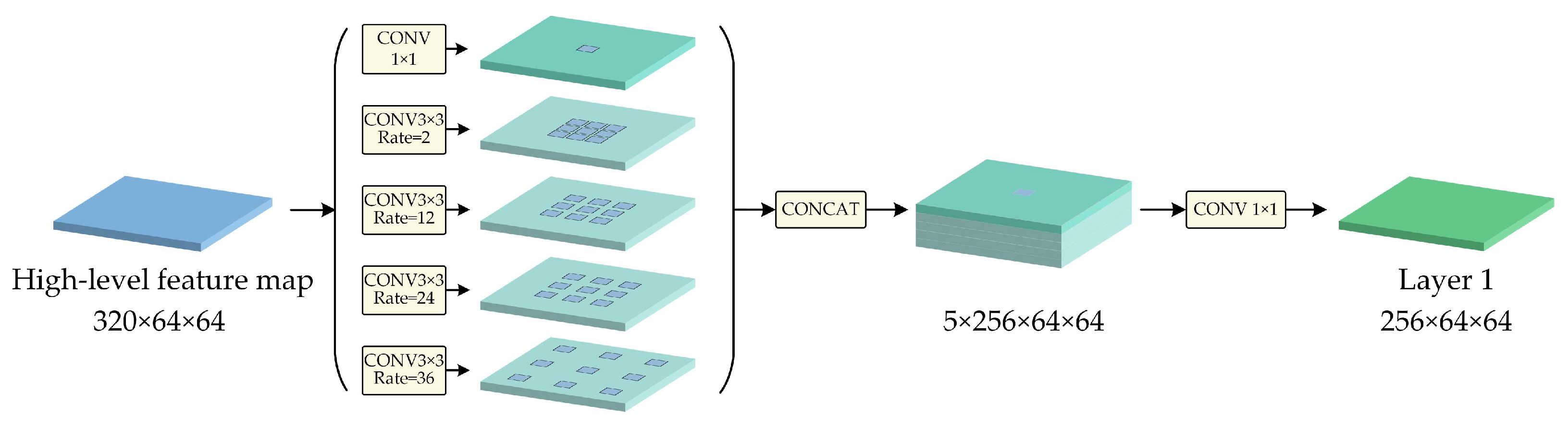
For feature maps, feature pyramids can be applied to enlarge their receptive fields and obtain multiscale target features. The pyramid scene parsing network (PSPNet) [23] fuses four different scales of feature maps in parallel via a pyramid pooling module, improving the network’s ability to obtain multiscale information. In DeepLabv3 [24], an atrous spatial pyramid pooling (ASPP) structure is adopted to enlarge the receptive fields and, thus, has a significant advantage in large object segmentation. To restore more building contour information, Xu [25] enhanced the combination of an encoder and a decoder based on a DeepLabv3+ [26] network embedded with an ASPP module.

(2)

For input images, skip connections are applied to fuse different levels of feature maps to obtain multilevel image features. The level of image features increases as the network layers deepen. Low-level features provide the basis for object category detection, and high-level features facilitate accurate segmentation and positioning. U-Net [27] uses long skip connections to integrate low-level features with high-level features and has high performance in medical image segmentation. Improved from U-Net, networks such as IEU-Net [28], HA U-Net [29] and EMU-CNN [30] have performed well. The MPRSU-Net [31] was constructed by combining long and short skip connections, alleviating the holes and fragmentary edges in the segmentation results obtained when extracting large buildings.

Researchers [32,33,34] have also considered both types of approaches and constructed new building segmentation models by combining feature pyramid modules and skip connections, notably enhancing the efficiency of the building extraction task and the generalization capacities of the developed models. Nevertheless, the majority of existing building extraction methods fail to address model applicability, resulting in considerable computational complexity and tedious parameter tuning steps. These problems limit their deployment in practical applications such as disaster/emergency response [35], damage assessment [36,37], and military reconnaissance [38] that require high algorithmic efficiency. Therefore, to facilitate the practical application of our method, we reduce the model complexity and propose a network with an “encoder-decoder” structure called MSL-Net, which is capable of obtaining and utilizing both multiscale and multilevel features, where “M” represents the prefix “multi”, “S” represents “scale”, “L” represents “level”, and “Net” represents “Network ”. The key contributions are as follows.

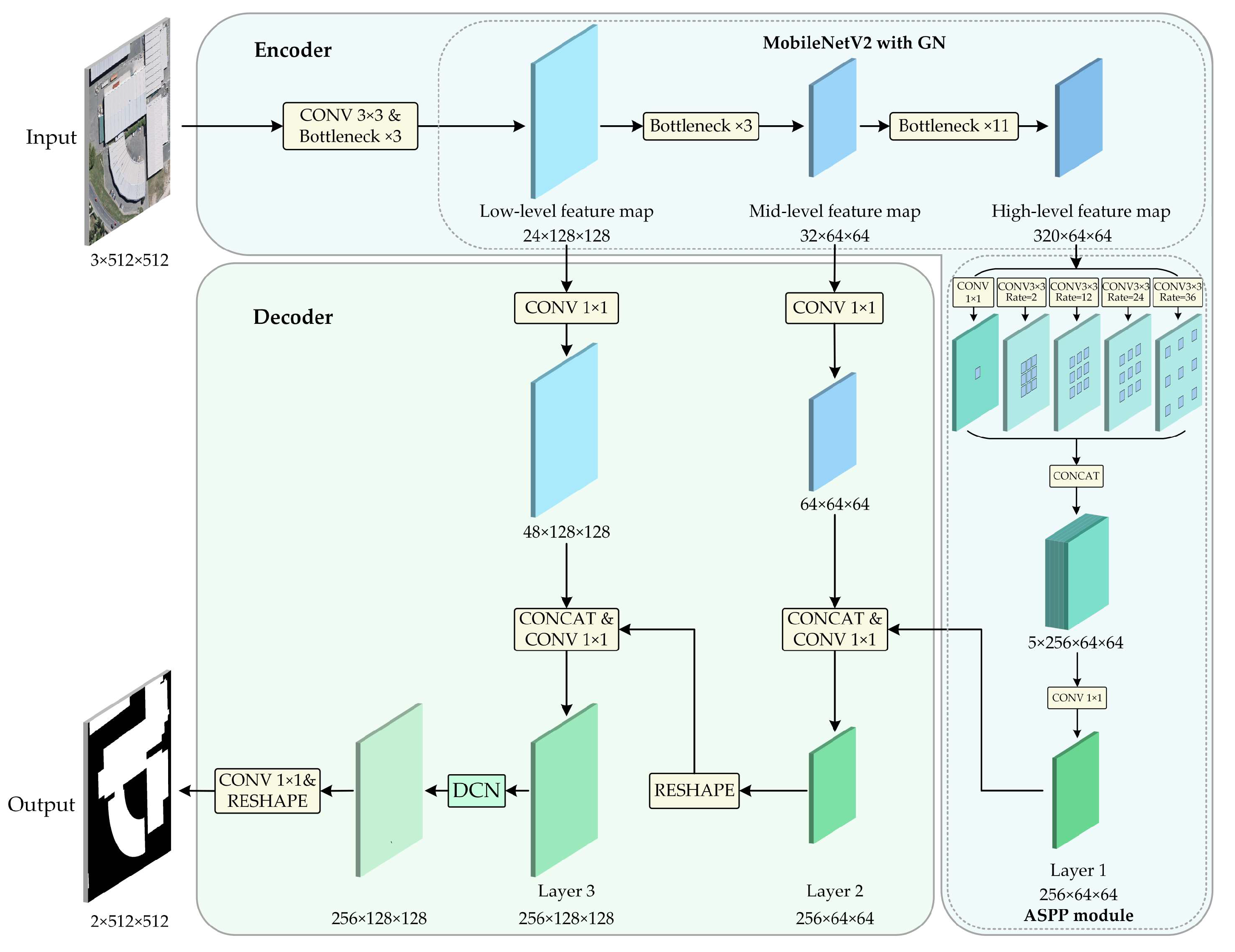
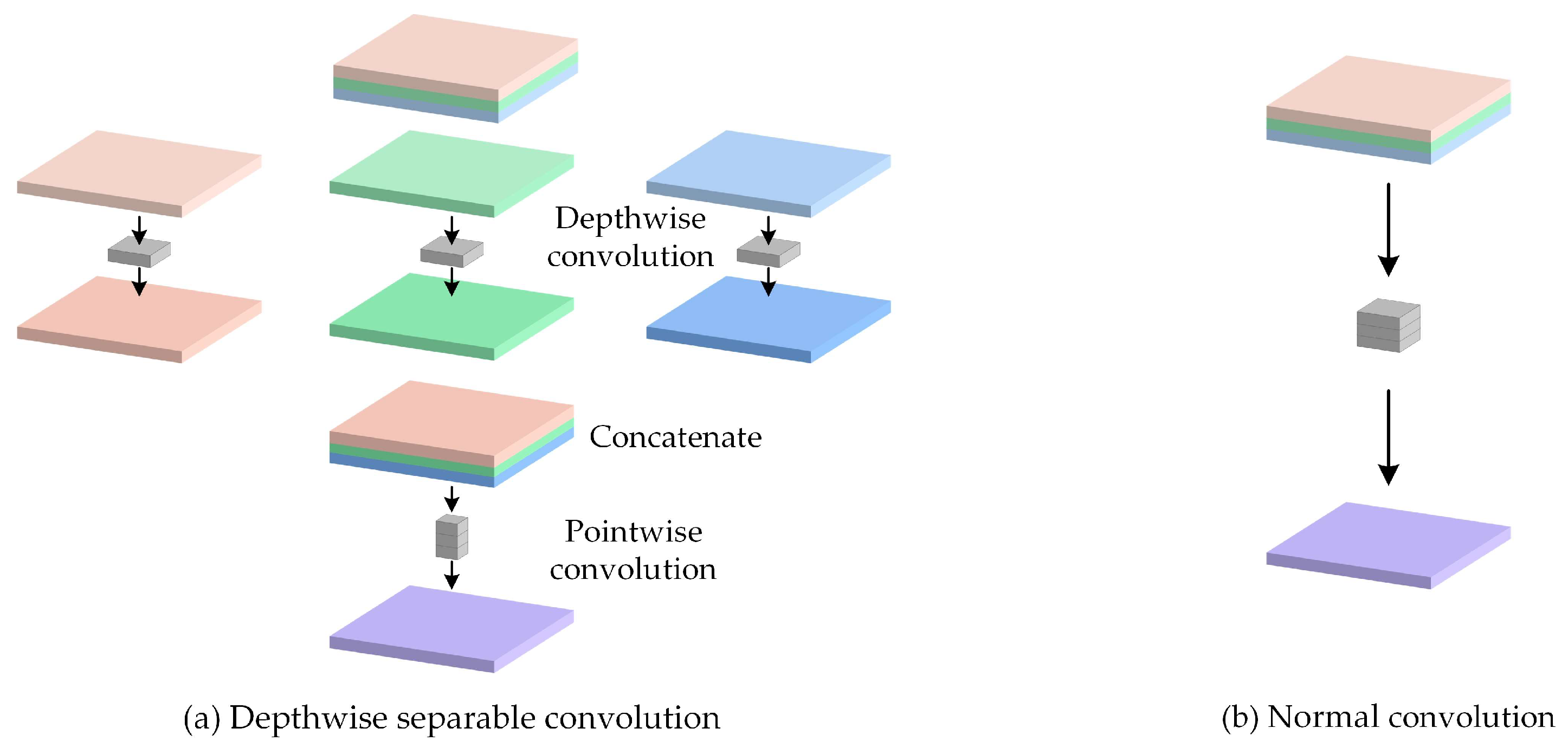
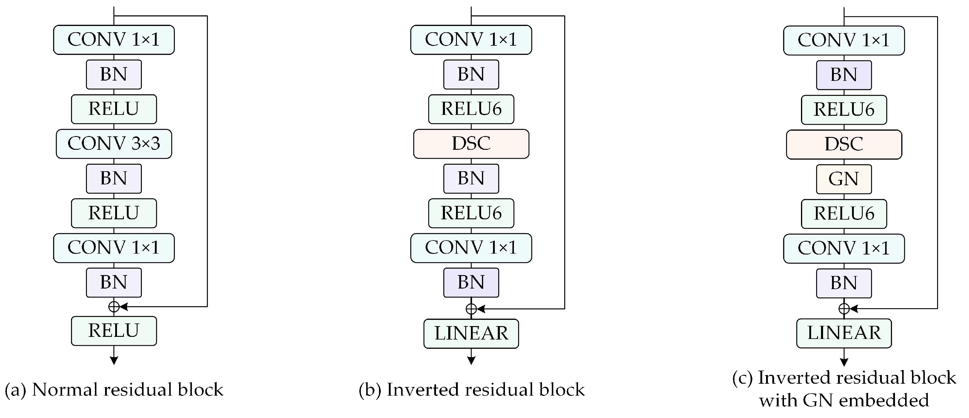
• In the encoding stage of MSL-Net, we introduce the MobileNetV2 [39] architecture to extract multilevel features. The inverted residual blocks in MobileNetV2 are constructed as bottlenecks using depthwise separable convolution (DSC) [40] and group normalization (GN) operations [41], which noticeably reduce the model complexity while improving its training and inference speeds. The multiscale features are extracted by an ASPP module to enhance the ability of the model to recognize multiscale buildings.
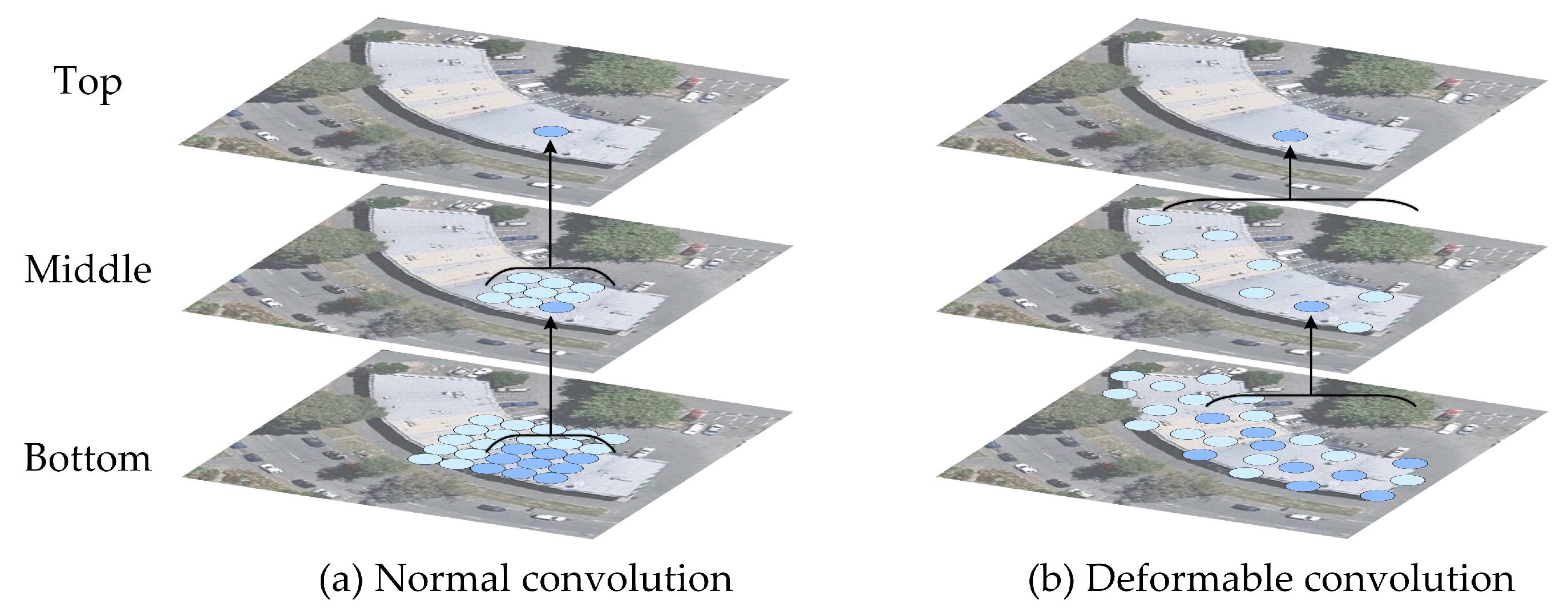
• In the decoding stage of MSL-Net, long skip connections [42] are applied to establish a long-distance dependence between the feature encoding and feature decoding layers. This long-distance dependence is beneficial for obtaining the rich hierarchical features of an image and effectively preventing holes in the segmentation results [31]. Before performing pixel classification, a deformable convolution network (DCN) layer [43] is added to ensure strong model robustness even when extracting buildings with irregular shapes.

2. Materials and Methods

2.1. MSL-Net Architecture

The encoder and decoder in MSL-Net are shown in Figure 1. The function of the encoder is to extract image features in a layer-by-layer manner. As the network layers gradually deepen, the feature map becomes more abstract; nonetheless, the extracted semantic information becomes richer, which is beneficial for classifying each pixel in the input image. In MSL-Net, the lightweight MobileNetV2 network with inverted residual blocks is introduced as the backbone to extract the original image features. We embed a GN layer in the inverted residual block, and three levels of feature maps with channels × height × width values of 24 × 128 × 128, 32 × 64 × 64, and 320 × 64 × 64 are output. Since the image downsampling operation during feature extraction lowers the feature map resolution and causes a partial loss of spatial information, the downsampling rate is limited to 8, and only three downsampling operations are performed. An ASPP module is used to extract multiscale features from the output high-level feature maps.

The decoder outputs prediction results with the same size as that of the original input image; these results are expressed as the final binary building segmentation map in the building semantic segmentation task. First, layer 1 is output by the ASPP module and concatenated with the mid-level feature map output by the backbone through a long skip connection. After the channels of the concatenated feature map are adjusted to 256 through a 1 × 1 convolution, we obtain layer 2. Second, layer 2 is resized by bilinear reshaping (denoted RESHAPE) to the same size as that of the low-level feature map extracted by the backbone, and then a concatenation operation (denoted CONCAT) and a 1 × 1 convolution (denoted CONV 1 × 1) are executed to obtain layer 3 with 256 channels and a size of 128 × 128. Thus far, multilevel image features and multiscale feature map features have been extracted. Third, the features of irregular building shapes are extracted through a DCN layer, whose output feature map has the same number of channels and size as its input feature map. Eventually, after a 1 × 1 convolution and a bilinear reshaping, a semantic segmentation image of the buildings with 2 channels and a size of 512 × 512 is output.

2.2. Feature Extraction Backbone in the Encoder

Typically, the deeper a network is, the richer the extracted features and the better the model performs. However, a deep learning model does not always perform better after simply stacking the layers of the network. Instead, the weight matrix may degrade, causing the network performance to deteriorate. The residual structure in ResNet [44] allows certain layers to be connected to each other through short skip connections, which weakens the strong correlation between two adjacent layers and mitigates network degradation. The inverted residual structure in the MobileNetV2 feature extraction backbone is based on the residual structure of ResNet, while the feature extraction sequence of “downscaling-convolution-upscaling” is changed to “upscaling-convolution-downscaling”, and the middle normal convolution is replaced by a DSC.

2.2.1. DSC in the Backbone

As shown in Figure 2, a DSC consists of two steps, a depthwise convolution and a pointwise convolution, which are performed separately in the spatial and channel dimensions to capture spatial information and fuse cross-channel depth information. Suppose that the input feature map size (length × width × channels) is D_F × D_F × M, the output feature map size is D_F × D_F × N, and the normal convolution kernel size is D_K × D_K × M. Then, the ratio of the number of DSC parameters to the number of normal convolution parameters is:

$$\frac{(D_K\times D_K\times 1)\times M+(1\times 1\times M)\times N}{(D_K\times D_K\times M)\times N}=\frac{1}{N}+\frac{1}{D_K^2}$$

(1)

which indicates that the DSC can exponentially reduce the required number of parameters, and this advantage becomes increasingly apparent as the number of layers increases.

2.2.2. GN in the Backbone

Batch normalization (BN) [45] has been widely used in existing deep learning algorithms. MobileNetV2 contains three BN layers in each inverted residual structure. Each BN layer takes the overall statistics for inference, imposing constraints on the search spaces of the system parameters, accelerating network convergence, and alleviating the overfitting problem. However, due to the stacking effect of BN in the network, the input distribution deviation between the training and test sets causes BN estimation bias to accumulate, which adversely affects the test performance of the model [46]. Note that GN can prevent the accumulation of such estimation bias. For this reason, we replace the second BN layer in the original inverted residual structure (shown in Figure 3c) with a GN layer to prevent network performance degradation due to distribution bias and ensure the robustness of the network.

The general feature normalization formula is,

$${\widehat{x}}_i=\frac{1}{{\sigma }_i}\left(x_i-{\mu }_i\right)$$

(2)

For two-dimensional images, x is a computed feature derived from the feature map, and i = (i_N, i_C, i_H, i_W) is a four-dimensional vector of features indexed in the following order: “batch axis, channel axis, spatial height axis, spatial width axis”. µ and σ are the mean and standard deviation, respectively, computed using the following equations:

$$\begin{array}{cc}{\mu }_i=\frac{1}{m}{\displaystyle \sum _{k\in S_i}}{x}_k,& {\sigma }_i=\sqrt{\frac{1}{m}{\displaystyle \sum _{k\in S_i}}{(x_k-{\mu }_i)}^2+\epsilon }\end{array},$$

(3)

where ε is a constant with a small value, S_i is the set of pixels used to compute the mean and standard deviation, and m is the size of S_i. Then, formally, the set of groups normalized computation sets is defined as,

$$S_i=\left\{k|k_N=i_N,\lfloor \frac{k_C}{C/G}\rfloor =\lfloor \frac{i_C}{C/G}\rfloor \right\}.$$

(4)

here, G and C are the numbers of groups and channels, respectively, and C/G is the number of channels in each group. $\lfloor ·\rfloor$ is the floor operation, and $\lfloor \frac{k_C}{C/G}\rfloor =\lfloor \frac{i_C}{C/G}\rfloor$ indicates that both indices i and k are in the same channel group, assuming that each channel group is stored sequentially along the channel axis. GN computes µ and σ along the spatial height axis, the spatial width axis and a group of C/G channels. Specifically, we use the same µ and σ to normalize the pixels in the same group.

2.3. ASPP in the Encoder

Atrous convolutions [47] introduce the concept of “dilation rates” based on the normal convolution, as shown in the ASPP module in Figure 4. Atrous convolutions with different dilation rates insert corresponding zero values into the normal convolution kernel to achieve convolution dilation, thereby increasing the receptive fields; this is similar to pooling operations. The scale features extracted by atrous convolutions with different dilation rates are also different. Additionally, since the inserted zero values are not calculated, the calculation counts do not increase, and the spatial resolution of the output feature maps does not decrease.

We replace the original ASPP branch with an atrous convolution possessing a dilation rate of 2 in our experiments. The ASPP module in MSL-Net concatenates and fuses the five feature maps output by a 1 × 1 convolution and four atrous convolutions with dilation rates of 2, 12, 24 and 36, obtaining both large-scale global information and small-scale local detail information. After a 1 × 1 convolution, the number of channels in the concatenated feature map is compressed to 256.

2.4. Deformable Convolution in the Decoder

Buildings in images are susceptible to different degrees of deformation due to external conditions such as the attitude of the equipment and weather conditions. In addition, due to the diversity of the shapes of buildings, a normal convolution has difficulty extracting the shape features of buildings, while a deformable convolution is able to adaptively adjust according to the deformation of the object in an image and efficiently extract robust features from objects with different shapes and directions.

Figure 5 depicts schematic diagrams of a normal convolution and a deformable convolution in the two-dimensional plane. Figure 5a represents the normal convolution, where the convolution kernel size is 3 × 3, and the sample points are organized in a regular pattern. Figure 5b represents the deformable convolution, where each sample point has position offsets, and the arrangement becomes irregular.

A normal two-dimensional convolution includes two steps: (1) sampling on the input feature mapping x with a normal convolution kernel K and (2) summing over the w-weighted sampled values. For each position p on the output feature mapping y,

$$y\left(p\right)=\sum _{k=1}^K{w}_k·x\left(p+p_k\right),$$

(5)

where k lists the positions in K.

In a deformable convolution, the position offsets are first obtained through a normal convolution layer, and then the offsets and magnitudes of the features learned from each sampling point are modulated. Finally, a more complex geometric transform feature learning process is performed, which is calculated as,

$$y\left(p\right)=\sum _{k=1}^K{w}_k·x\left(p+p_k+\Delta p_k\right)·\Delta m_k,$$

(6)

where ∆p_k and ∆m_k represent the learnable offset and weight scalar at position k, respectively. ∆m_k represents the modulation scalar at position k in the range [0, 1], and the calculation of the offset value is executed using bilinear interpolation. ∆p_k and ∆m_k can be obtained by applying a convolution to the same input feature map layer. The number of output channels is 3K, and K represents the convolutional kernel size of the backbone. The first 2K dimensions represent the x and y offsets (∆p_k) at each position, and the subsequent K dimensions are used to obtain the weight (∆m_k) of each position according to the sigmoid layer.

We add a deformable convolution layer to enhance the feature extraction ability of our model for geometric shapes before the final pixel classification output of the network.

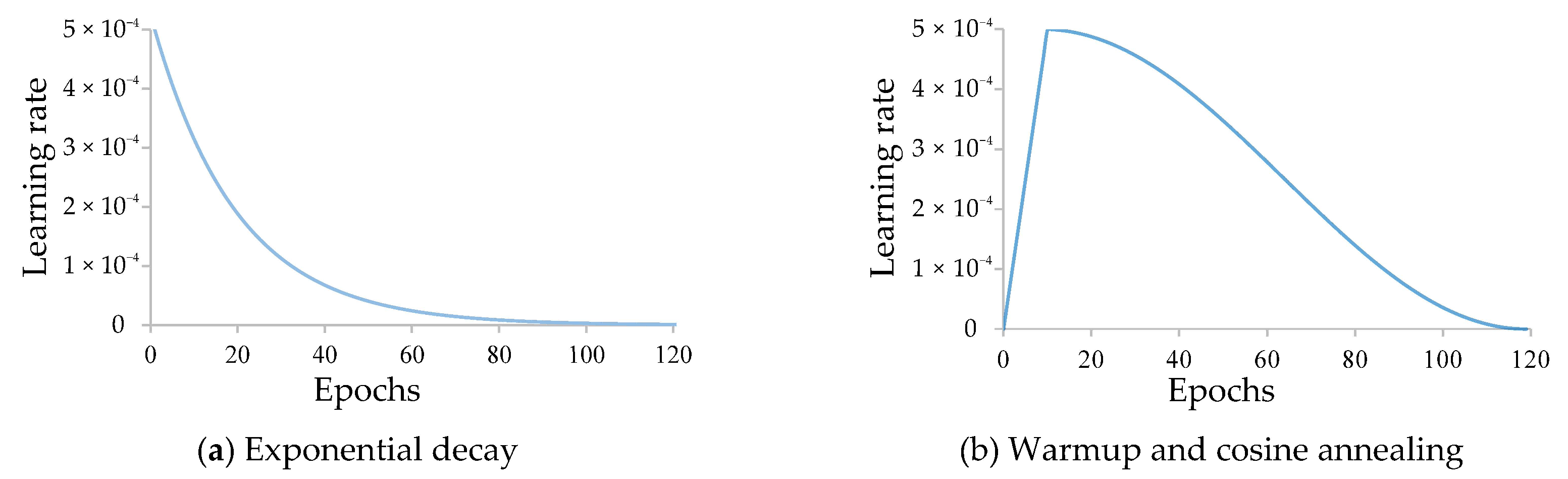
2.5. Warmup and Cosine Annealing Learning Rate Policy

During training, gradient descent is usually adopted to optimize models. The learning rate (LR) is one of the hyperparameters that affect the model optimization process; it plays a guiding role in how to use the loss function gradient to adjust the network weights in the gradient descent step. When model training starts, a large initial LR is generally set to rapidly decrease the loss value of the network, and the LR decreases in a certain way as the number of iterations increases to ensure small model fluctuations during the later training stages as it gradually approaches the global optimal solution. The LR usually decreases via exponential decay, piecewise constant decay, or cosine annealing [48].

Since the network is relatively unstable in the early training stage, a large initial LR causes the gradient of the weights to fluctuate back and forth, and a small initial LR decelerates network convergence; thus, we employ the “warmup and cosine annealing” LR policy to ensure the performance of the model. As shown in Figure 6b, in the first 10 epochs, the LR linearly increases from 0 to the base LR and then gradually decreases from the base LR to 0 as the number of epochs increases. The LR is calculated by:

$${\eta }_{\mathrm{t}}=\{\begin{array}{ll}\frac{{\eta }_{\max }{T}_{\mathrm{cur}}}{T_{\mathrm{wu}}},\hfill & T_{\mathrm{cur}}\le T_{\mathrm{wu}}\hfill \\ \frac{{\eta }_{\max }}{2}\left(1+\cos \left(\frac{T_{\mathrm{cur}}-T_{\mathrm{wu}}}{T_{\max }}\pi \right)\right),\hfill & T_{\mathrm{wu}}<T_{\mathrm{cur}}\le T_{\max }\hfill \end{array},$$

(7)

where η_t is the LR of the current training epoch, η_max is the base LR, T_cur is the current number of training epochs, T_wu is the total number of warmup epochs, and T_max is the maximum number of training epochs.

3. Experiments and Results

3.1. Descriptions of the Datasets

In this study, we use the WHU Building Aerial Imagery dataset (WHU dataset) [3], Inria Aerial Image Labeling dataset (Inria dataset) [49], and Massachusetts Buildings dataset (Massachusetts dataset) [50], with spatial resolutions ranging from 0.3 m to 1.0 m; thus, we can fully test the performance of the developed model. The details of each dataset are listed in

Table 1. Details of each dataset.

Dataset	Spatial Resolution (m)	Pixels	Area (km2)	Tiles
WHU dataset	0.3	512 × 512	450	8189
Inria dataset	0.3	5000 × 5000	810	180
Massachusetts dataset	1.0	1500 × 1500	240	151

.

For both the Massachusetts dataset and the WHU dataset, the training and validation steps are performed directly using the training, validation, and test set ratios that have been partitioned by default in these datasets. For the Inria dataset, the training, validation, and test sets are divided at a ratio of 8:1:1. The numbers of images in the training, validation and test sets used for each dataset in the experiments are shown in

Table 2. Division of each dataset.

Dataset	Training Set	Validation Set	Test Set
WHU dataset	4737	1036	2416
Inria dataset	14418	1782	1800
Massachusetts dataset	1233	36	90

.

3.2. Experimental Settings

The main software and hardware used in our study are listed in

Table 3. Details of the employed hardware and software.

Item	Details
CPU	Intel i7-12700K @ 3.61 GHz
GPU	GeForce RTX 3090 (24 GB)
OS	Windows 10 x64
Language	Python 3.8
Framework	PyTorch 1.8.1

.

Since buildings are the only experimental objects, the pixel value range of the labeled binary map is adjusted from [0, 255] to [0, 1] before training, where pixels with values of 1 represent the buildings and pixels with values of 0 represent the background. The widely used and high-performing U-Net, PSPNet, and DeepLabv3+ are selected for comparison, and all four models are tested on the above three datasets using the same training, validation, and test sets. The input images are one-hot coded, the batch size is set to 12, the loss function is a direct summation of the focal loss [51] and dice loss [52], the Adam optimizer is used in the training process, the base LR is set to 0.0005, and each comparison model is trained for 120 epochs using an exponential decay LR policy with a gamma value of 0.0005. MSL-Net is first warmed up for 10 epochs and then trained for 110 epochs using the cosine annealing LR policy.

In the training stage, data augmentation strategies are applied to preprocess the input images to obtain more feature information from the limited data. Due to the rich geometric features of the buildings in the dataset, we first apply spatial data augmentation strategies, including random horizontally mirror flipping with a 50% probability, random rotation with 50% probabilities at different angles (−10° to 10°), and random scaling with ratios between 0.25 and 2. Then, spectral data augmentation strategies are applied to reduce the impact caused by imaging condition differences to improve the generalization ability of the network. The spectral data augmentation techniques include hue augmentation, saturation augmentation, value augmentation and random Gaussian blurring.

3.3. Evaluation Metrics

To quantitatively evaluate the reliability and accuracy of each model, we use six metrics, the Intersection-Over-Union (IoU), F1-score, Accuracy, Recall, Precision and Kappa, to evaluate the segmentation results. The building segmentation results are compared with the corresponding building labels at the pixel level, and the instances are classified as positive or negative, with true indicating a correct prediction and false indicating an incorrect prediction; thus, true positives (TPs) represent the correctly predicted building pixels, false positives (FPs) represent the pixels that predict the background as buildings, false negatives (FNs) represent the pixels that predict buildings as the background, and true negatives (TNs) represent the correctly predicted background pixels. The confusion matrix is shown in

Table 4. Confusion matrix.

	Prediction	Building	Background
Ground Truth
Building		TP	FN
Background		FP	TN

.

Among these six metrics, Recall denotes the proportion of correctly predicted building pixels among all real building pixels, Precision denotes the proportion of correctly predicted building pixels among all predicted building pixels, and the IoU, which is currently the most commonly used evaluation metric in semantic segmentation tasks, denotes the ratio of the intersection to the union of the predicted building and real building pixels. Accuracy indicates the proportion of correctly predicted pixels among all pixels. The F1-score is the harmonic mean of the Recall and Precision. Kappa is a metric that considers both the target and background accuracies. The Recall, Precision, IoU, Accuracy, F1-score and Kappa are defined as:

Recall = TP/(FN + TP),

(8)

Precision = TP/(FP + TP),

(9)

IoU = TP/(FN + FP + TP),

(10)

Accuracy = (TP + TN)/(FP + FN + TP + TN),

(11)

F1-score = 2TP/(2TP + FN + FP),

(12)

P₀ = (TP + FP)/(FP + FN + TP + TN),

(13)

P_e = ((TP + FN)(TP + FP) + (FN + TN)(FP + TN))/((FP + FN + TP + TN)²),

(14)

Kappa = (P₀ − P_e)/(1 − P_e).

(15)

4. Discussion

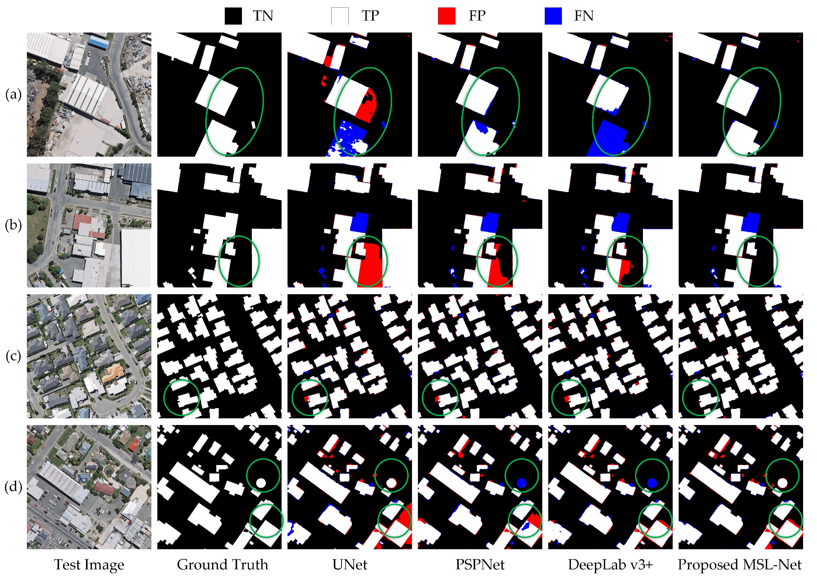
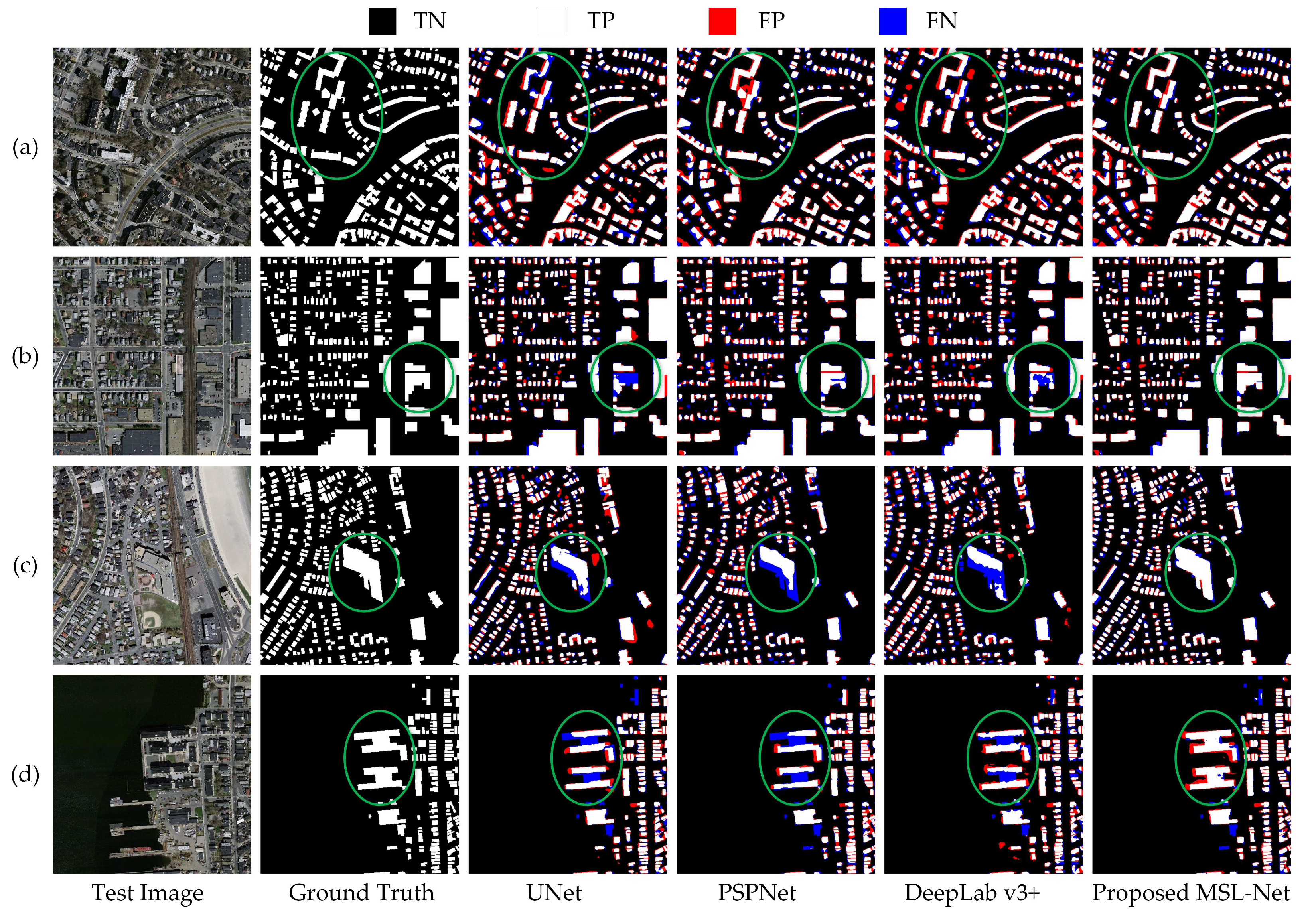
4.1. Comparisons on Each Dataset

4.1.1. Comparison on the WHU Dataset

The WHU dataset is the most accurate building dataset available to date [53]; it consists of aerial images of Christchurch, New Zealand, with extraordinarily high image resolutions. Building images with obvious spectral features, geometric features, and spatial distribution features are selected from the dataset for display, as shown in Figure 7, where white pixels indicate the correctly detected parts of a building, red pixels indicate incorrectly detected parts of a building, blue pixels indicate the missed parts of a building, and black pixels indicate the correctly detected background.

In Figure 7a, U-Net, PSPNet, and DeepLabv3+ all fail to detect large bungalows to some degree, and some results have rough building edges with some discrete pixels, whereas MSL-Net decreases the salt and pepper noise by fusing multiscale and multilevel features through its ASPP module and long skip connections. In Figure 7b, the other three methods have varying degrees of false detection. This is because the building roofs are similar to the ground in terms of color and texture, which signifies “intraclass spectral heterogeneity”. The results of Figure 7b demonstrate that MSL-Net effectively reduces the negative impact of “intraclass spectral heterogeneity” on the extraction of buildings and achieves enhanced recognition accuracy. Figure 7c depicts a region with a significant number of densely distributed small-scale buildings, and MSL-Net efficiently mitigates false detection. Buildings of various sizes and shapes can be found in Figure 7d. According to the extraction results, U-Net and PSPNet are unable to effectively discriminate between the ground and buildings. Buildings with irregular shapes, such as round buildings, are ineffectively extracted by PSPNet and DeepLabv3+. MSL-Net not only eliminates the negative impact of “intraclass spectral heterogeneity” but also completely extracts round buildings and maintains their continuity, revealing that the deformable convolutional layer is involved in the detection of target features with irregular shapes.

To quantitatively evaluate the extraction effect of each method, the results of each metric are calculated, as shown in

Table 5. Metrics produced on the WHU dataset. The highest scores are bolded; the second-highest scores are underlined.

Method	IoU (%)	Accuracy (%)	F1-Score (%)	Kappa (%)	Precision (%)	Recall (%)
U-Net	84.9	98.2	91.9	90.8	90.0	93.8
PSPNet	87.6	98.5	93.4	92.6	92.6	94.3
DeepLabv3+	88.0	98.6	93.6	92.8	94.4	92.9
MSL-Net	90.4	98.9	95.0	94.3	95.1	94.8

.

In Table 5, MSL-Net exceeds 90% in every metric, with IoU, F1-score and Kappa values that are about 2.4%, 1.4% and 1.5% higher than those of the second-best model, respectively. Our proposed model outperforms the widely used models in accuracy of recognition outcomes.

4.1.2. Comparison on the Inria Dataset

The Inria dataset comprises a variety of urban landscapes, covering an area of 810 km² in 10 different cities. Various places have diverse architectural types, and the spectral features and shadow features of the images also vary depending on their imaging times and meteorological conditions, so this dataset might be a good indicator of a model’s robustness in different scenarios. Some of the original images and labels and the corresponding results extracted by each method are shown in Figure 8.

The spatial distribution of the buildings in Figure 8a is uneven, and the materials and spectral features of the roofs of the scattered buildings vary. The buildings in Figure 8b are large in scale and are connected by several buildings with different spectral features. The building structures are complex, and shadows obscure the buildings. Figure 8c contains two types of buildings, villas and large bungalows, and the spectral features of the buildings and the ground are relatively similar. The buildings in Figure 8d are rectangular ambulatory planes in terms of shape, and the spectral features of the roofs are complex.

MSL-Net effectively reduces the amount of missed detection and effectually suppresses the occurrence of false detection, as shown in Figure 8a,c. Figure 8b shows how MSL-Net successfully distinguishes rooftops and road surfaces with similar spectral features, weakening the influence of the “interclass spectral homogeneity”. MSL-Net also effectively distinguishes between white and brown rooftops with different spectral features and successfully extracts white buildings shaded by trees, indicating that MSL-Net can reduce the impact of shaded buildings to some extent. We can observe in Figure 8b,d that MSL-Net can recognize buildings with complicated structures.

Table 6. Metrics produced on the Inria dataset. The highest scores are bolded; the second-highest scores are underlined.

Method	IoU (%)	Accuracy (%)	F1-Score (%)	Kappa (%)	Precision (%)	Recall (%)
U-Net	78.2	96.2	87.8	85.5	88.5	87.0
PSPNet	80.9	96.7	89.4	87.5	88.9	89.9
DeepLabv3+	78.1	96.2	87.7	85.4	88.2	87.1
MSL-Net	81.1	96.8	89.6	87.7	89.3	89.9

lists the computed evaluation metric results. The IoU, F1-score and Kappa coefficient of MSL-Net are 0.2%, 0.2% and 0.2% higher than those of the second-best model PSPNet, respectively; these results are not much higher than those of the PSPNet, but they still indicate that MSL-Net has good competitiveness in the building recognition task in various situations.

4.1.3. Comparison on the Massachusetts Dataset

The Massachusetts dataset includes Boston aerial images with 1-m spatial resolutions, which are significantly lower than the 0.3-m resolutions of the WHU dataset and Inria dataset. With these lower spatial resolutions, the feature information of buildings is rough and more difficult to extract. Some of the original images and labels and the corresponding results extracted by each method are shown in Figure 9.

In general, most of the buildings in the segmentation results are displayed in fragmented patchy distributions, which greatly test each model’s ability to extract small targets. Figure 9a,b demonstrate that MSL-Net can alleviate the occurrences of missed and false detections to a certain extent, and Figure 9c,d demonstrate that MSL-Net is also able to effectively identify irregular buildings.

The results of the calculated evaluation metrics are shown in

Table 7. Metrics produced on the Massachusetts dataset. The highest scores are bolded; the second-highest scores are underlined.

Method	IoU (%)	Accuracy (%)	F1-Score (%)	Kappa (%)	Precision (%)	Recall (%)
U-Net	67.6	92.6	80.7	76.1	78.5	83.0
PSPNet	67.2	92.6	80.4	75.8	79.3	81.5
DeepLabv3+	63.3	91.3	77.5	74.5	74.9	80.4
MSL-Net	70.9	93.6	83.0	79.0	81.9	84.1

. The IoU, F1-score and Kappa coefficient values of MSL-Net are 3.3%, 2.3% and 2.9% higher than those of the second-best model U-Net, respectively, and all other metrics are also better. The results show that MSL-Net still has strong robustness even when working with images possessing poor spatial resolutions.

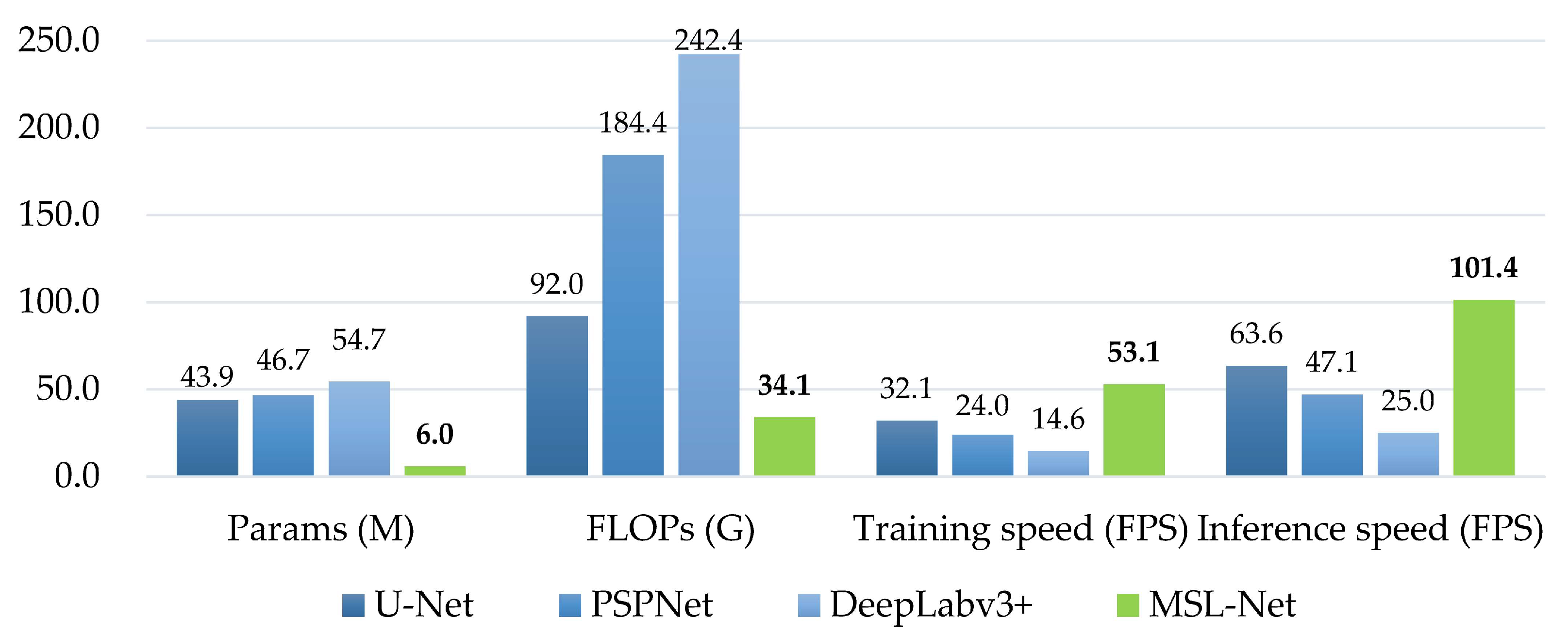
4.2. Complexity Comparison

Complexity is a critical factor that affects the practical application of a model. In the building extraction task based on the CNN method, lower numbers of parameters and floating-point operations (FLOPs) often result in faster training and inference speeds. A model with lower complexity is more convenient for practical applications. To objectively evaluate the complexity of each model, the number of parameters, the number of FLOPs, the training speed and the inference speed are calculated separately for each model. On an NVIDIA RTX 3090 GPU, the training speed is expressed as the number of frames per second (FPS) required for an input image of size 3 × 512 × 512, and the inference speed is expressed as the number of FPS required for 2 input images of size 3 × 512 × 512. The quantitative comparison results are shown in Figure 10.

In Figure 10, we can easily find that MSL-Net obviously achieves the fastest training speed and inference speed with very small numbers of parameters and FLOPs. In detail, the numbers of parameters and FLOPs required by MSL-Net are much lower than those of DeepLabv3+ and PSPNet, which are approximately 14% and 37% of the numbers required by the suboptimal U-Net model, respectively. Our proposed MSL-Net reaches a competitive training speed of 53.1 FPS, which is 65% faster than that of the second-best model, while the inference speed surpasses those of other models by more than 57.1% with an FPS of 101.4.

4.3. Comparison with State-of-the-Art Methods

To verify the effectiveness of the proposed network, MSL-Net is compared with recent state-of-the-art building extraction methods, including AGs-Unet [54], PISANet [55], DR-Net [56], RSR-Net [57], BRRNet [58], and SRI-Net [59], on the accurate WHU dataset. As WHU dataset is a publicly available dataset, we use the reported model performances for our comparisons. The quantitative comparison results are shown in

Table 8. Comparison with state-of-the-art methods on the WHU dataset. Here, ‘–’ denotes that the paper did not provide relevant data. The best results are bolded; the second-best results are underlined.

Method	IoU (%)	F1-Score (%)	Params (M)
AGs-Unet	85.5	–	34.9
PISANet	88.0	93.6	–
DR-Net	88.3	93.8	9.0
RSR-Net	88.3	–	2.9
BRRNet	89.0	94.1	17.3
SRI-Net	89.1	94.2	–
MSL-Net	90.4	95.0	6.0

.

As seen in Table 8, the IoU and F1-score of MSL-Net are superior to those of all the tested methods that have been developed in recent studies, demonstrating the state-of-the-art performance of our proposed method. Compared with RSR-Net, BRRNet, and SRI-Net, our proposed MSL-Net achieves IoU improvements of 2.1%, 1.4%, and 1.3% on the WHU dataset, respectively. MSL-Net also achieves competitive number of parameters, demonstrating its great tradeoff between complexity and accuracy.

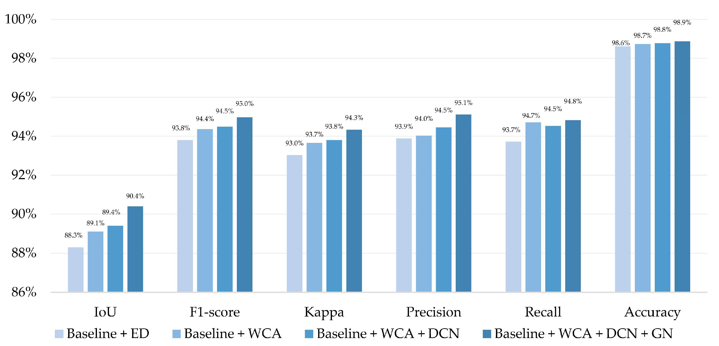
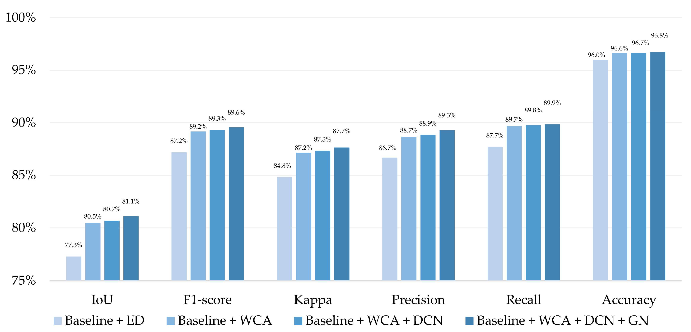
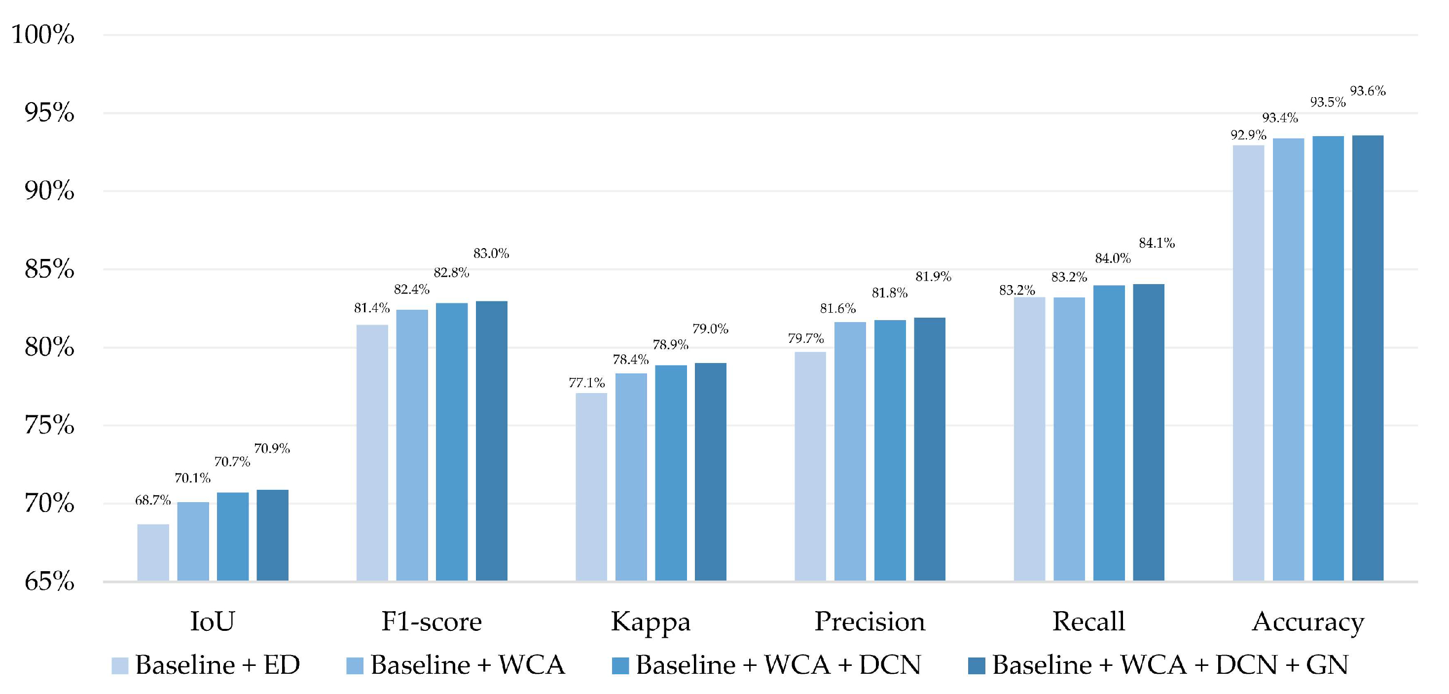
4.4. Ablation Experiments

To verify the effectiveness of each improvement, we perform ablation experiments on the WHU dataset, Inria dataset and Massachusetts dataset. Based on the baseline (MSL-Net with the unimproved MobileNetV2), we first change the LR policy from exponential decay (ED) to warmup and cosine annealing (WCA), and then we add a DCN layer at the end of the network. Finally, we replace the second BN layer with a GN layer in the inverse residual structure. The results of the six metrics are calculated, as shown in

Table 9. Ablation experimental results obtained on the three datasets. The highest scores are bolded; the second-highest scores are underlined.

Method	WHU		Inria		Massachusetts
	IoU	F1-Score	IoU	F1-Score	IoU	F1-Score
Baseline + ED	88.3%	93.9%	77.3%	87.2%	68.7%	81.4%
Baseline + WCA	89.1%	94.6%	80.5%	89.2%	70.1%	82.4%
Baseline + WCA + DCN	89.4%	94.9%	80.7%	89.3%	70.7%	82.8%
Baseline + WCA + DCN + GN	90.4%	95.0%	81.1%	89.6%	70.9%	83.0%

and Figure 11, Figure 12 and Figure 13.

The metrics of the model demonstrate constant trends toward superiority with the adjustment of the LR policy, the addition of the DCN, and the embedding of GN in the inverse residual module. For instance, on the WHU dataset, the WCA increases the IoU by 0.8% and the F1-score by 0.7%, the DCN module increases the IoU by 0.3% and the F1-score by 0.3%, and the improvement of the inverse residual structure increases the IoU by 1.0% and the F1-score by 0.1%. The ablation experimental results strongly prove the effectiveness of our introduced improvements.

4.5. Limitations and Future Work

Despite superior performance achieved by the proposed MSL-Net in accuracy and complexity, MSL-Net still has limitations that need to be addressed. The experimental results of MSL-Net on the Inria dataset with more complex scenes have insignificant advantages over those of PSPNet, and it is still necessary to strengthen the robustness of lightweight MSL-Net in complex scenes. Additionally, the number of parameters of the ASPP module accounts for a large proportion of that of the whole network. In future work, the improvements or replacements of the ASPP module can be considered to address this limitation.

5. Conclusions

In this paper, we propose MSL-Net, an efficient neural network for building extraction. In terms of its network structure, MSL-Net adopts an ASPP module and skip connections to obtain the multiscale features of buildings and the multilevel features of images. The numbers of network parameters and computations are reduced by a DSC, GN is embedded in the inverted residual structure to alleviate network degradation, and the extraction capability of the model for irregularly shaped buildings is ensured by a DCN layer. Experiments are conducted on three publicly available datasets with varying spatial resolutions and building styles, and MSL-Net outperforms the comparison methods in model accuracy, demonstrating its superiority and robustness. Complexity evaluation experiments reveal that MSL-Net surpasses other models by more than 57.1% with an inference speed of 101.4 FPS; it requires only 14% of the parameters and 37% of the FLOPs required by the second-best method, manifesting the efficiency of MSL-Net. Ablation experiments indicate the effectiveness of each improvement. However, we find that the experimental results obtained by MSL-Net on the Inria dataset with more complex scenes are not sufficiently superior, and we will focus on enhancing the robustness of MSL-Net to complex scenes in our future work so that MSL-Net can perform well when monitoring urbanization in different cities.

References

1. Zeng, Y.; Guo, Y.; Li, J. Recognition and Extraction of High-Resolution Satellite Remote Sensing Image Buildings Based on Deep Learning. Neural. Comput. Appl. 2022, 34, 2691–2706. [Google Scholar] [CrossRef]
2. Ghanea, M.; Moallem, P.; Momeni, M. Building Extraction from High-Resolution Satellite Images in Urban Areas: Recent Methods and Strategies Against Significant Challenges. Int. J. Remote Sens. 2016, 37, 5234–5248. [Google Scholar] [CrossRef]
3. Ji, S.; Wei, S.; Lu, M. Fully Convolutional Networks for Multisource Building Extraction from an Open Aerial and Satellite Imagery Data Set. IEEE Trans. Geosci. Remote Sens. 2019, 57, 574–586. [Google Scholar] [CrossRef]
4. Chen, Q.; Wang, L.; Waslander, S.L.; Liu, X. An End-to-End Shape Modeling Framework for Vectorized Building Outline Generation from Aerial Images. ISPRS J. Photogramm. Remote Sens. 2020, 170, 114–126. [Google Scholar] [CrossRef]
5. Katartzis, A.; Sahli, H.; Nyssen, E.; Cornelis, J. Detection of Buildings from a Single Airborne Image Using a Markov Random Field Model. In Proceedings of the IGARSS 2001, Scanning the Present and Resolving the Future, IEEE 2001 International Geoscience and Remote Sensing Symposium (Cat. No.01CH37217), Sydney, Australia, 9–13 July 2001; Volume 6, pp. 2832–2834. [Google Scholar]
6. Simonetto, E.; Oriot, H.; Garello, R. Rectangular Building Extraction from Stereoscopic Airborne Radar Images. IEEE Trans. Geosci. Remote Sens. 2005, 43, 2386–2395. [Google Scholar] [CrossRef]
7. Jung, C.R.; Schramm, R. Rectangle Detection Based on a Windowed Hough Transform. In Proceedings of the 17th Brazilian Symposium on Computer Graphics and Image Processing, Curitiba, Brazil, 20–20 October 2004; pp. 113–120. [Google Scholar]
8. Li, L. Research on Shadow-Based Building Extraction from High Resolution Remote Sensing Images. Master’s Thesis, Hunan University of Science and Technology, Xiangtan, China, 2011. [Google Scholar]
9. Zhao, Z.; Zhang, Y. Building Extraction from Airborne Laser Point Cloud Using NDVI Constrained Watershed Algorithm. Acta Optica Sin. 2016, 36, 503–511. [Google Scholar]
10. Zhou, S.; Liang, D.; Wang, H.; Kong, J. Remote Sensing Image Segmentation Approach Based on Quarter-Tree and Graph Cut. Comput. Eng. 2010, 36, 224–226. [Google Scholar]
11. Wei, D. Research on Buildings Extraction Technology on High Resolution Remote Sensing Images. Master’s Thesis, Information Engineering University, Zhengzhou, China, 2013. [Google Scholar]
12. Tournaire, O.; Brédif, M.; Boldo, D.; Durupt, M. An Efficient Stochastic Approach for Building Footprint Extraction from Digital Elevation Models. ISPRS J. Photogramm. Remote Sens. 2010, 65, 317–327. [Google Scholar] [CrossRef]
13. Parsian, S.; Amani, M. Building Extraction from Fused LiDAR and Hyperspectral Data Using Random Forest Algorithm. Geomatica 2017, 71, 185–193. [Google Scholar] [CrossRef]
14. Ferro, A.; Brunner, D.; Bruzzone, L. Automatic Detection and Reconstruction of Building Radar Footprints from Single VHR SAR Images. IEEE Trans. Geosci. Remote Sens. 2013, 51, 935–952. [Google Scholar] [CrossRef]
15. Wei, Y.; Zhao, Z.; Song, J. Urban Building Extraction from High-Resolution Satellite Panchromatic Image Using Clustering and Edge Detection. In Proceedings of the IEEE International Geoscience and Remote Sensing Symposium, Anchorage, AK, USA, 20–24 September 2004; IEEE: Anchorage, AK, USA, 2004; Volume 3, pp. 2008–2010. [Google Scholar]
16. Huang, X.; Zhang, L. Morphological Building/Shadow Index for Building Extraction from High-Resolution Imagery Over Urban Areas. IEEE J. Sel. Top. Appl. Earth Obs. Remote Sens. 2012, 5, 161–172. [Google Scholar] [CrossRef]
17. Gao, X.; Wang, M.; Yang, Y.; Li, G. Building Extraction from RGB VHR Images Using Shifted Shadow Algorithm. IEEE Access 2018, 6, 22034–22045. [Google Scholar] [CrossRef]
18. Maruyama, Y.; Tashiro, A.; Yamazaki, F. Use of Digital Surface Model Constructed from Digital Aerial Images to Detect Collapsed Buildings during Earthquake. Procedia Eng. 2011, 14, 552–558. [Google Scholar] [CrossRef]
19. Guo, H.; Du, B.; Zhang, L.; Su, X. A Coarse-to-Fine Boundary Refinement Network for Building Footprint Extraction from Remote Sensing Imagery. ISPRS J. Photogramm. Remote Sens. 2022, 183, 240–252. [Google Scholar] [CrossRef]
20. Long, J.; Shelhamer, E.; Darrell, T. Fully Convolutional Networks for Semantic Segmentation. In Proceedings of the IEEE Conference on Computer Vision and Pattern Recognition, Boston, MA, USA, 7–12 June 2015; pp. 3431–3440. [Google Scholar]
21. Yuan, J. Learning Building Extraction in Aerial Scenes with Convolutional Networks. IEEE Trans. Pattern Anal. Mach. Intell. 2018, 40, 2793–2798. [Google Scholar] [CrossRef] [PubMed]
22. Maggiori, E.; Tarabalka, Y.; Charpiat, G.; Alliez, P. High-Resolution Aerial Image Labeling with Convolutional Neural Networks. IEEE Trans. Geosci. Remote Sens. 2017, 55, 7092–7103. [Google Scholar] [CrossRef]
23. Zhao, H.; Shi, J.; Qi, X.; Wang, X.; Jia, J. Pyramid Scene Parsing Network. In Proceedings of the IEEE Conference on Computer Vision and Pattern Recognition, Honolulu, HI, USA, 21–26 July 2017; pp. 2881–2890. [Google Scholar]
24. Chen, L.-C.; Papandreou, G.; Schroff, F.; Adam, H. Rethinking Atrous Convolution for Semantic Image Segmentation. arXiv 2017, arXiv:1706.05587. [Google Scholar]
25. Xu, Z.; Shen, Z.; Li, Y.; Zhao, L.; Ke, Y.; Li, L.; Wen, Q. Classification of High-Resolution Remote Sensing Images Based on Enhanced DeepLab Algorithm and Adaptive Loss Function. Nat. Remote Sens. Bull. 2022, 26, 406–415. [Google Scholar]
26. Chen, L.-C.; Zhu, Y.; Papandreou, G.; Schroff, F.; Adam, H. Encoder-Decoder with Atrous Separable Convolution for Semantic Image Segmentation. In Proceedings of the European Conference on Computer Vision (ECCV), Munich, Germany, 8–14 September 2018; pp. 833–851. [Google Scholar]
27. Ronneberger, O.; Fischer, P.; Brox, T. U-Net: Convolutional Networks for Biomedical Image Segmentation. In Proceedings of the Medical Image Computing and Computer-Assisted Intervention—MICCAI 2015, Munich, Germany, 5–9 October 2015; pp. 234–241. [Google Scholar]
28. Wang, Z.; Zhou, Y.; Wang, S.; Wang, F.; Xu, Z. House Building Extraction from High-Resolution Remote Sensing Images based on IEU-Net. Nat. Remote Sens. Bull. 2021, 25, 2245–2254. [Google Scholar]
29. Xu, L.; Liu, Y.; Yang, P.; Chen, H.; Zhang, H.; Wang, D.; Zhang, X. HA U-Net: Improved Model for Building Extraction from High Resolution Remote Sensing Imagery. IEEE Access 2021, 9, 101972–101984. [Google Scholar] [CrossRef]
30. Liu, Y.; Chen, D.; Ma, A.; Zhong, Y.; Fang, F.; Xu, K. Multiscale U-Shaped CNN Building Instance Extraction Framework with Edge Constraint for High-Spatial-Resolution Remote Sensing Imagery. IEEE Trans. Geosci. Remote Sens. 2021, 59, 6106–6120. [Google Scholar] [CrossRef]
31. Zhang, Y.; Yan, Q.; Deng, F. Multi-Path RSU Network Method for High-Resolution Remote Sensing Image Building Extraction. Acta Geod. Cartogr. Sin. 2022, 51, 135–144. [Google Scholar]
32. Xu, J.; Liu, W.; Shan, H.; Shi, J.; Li, E.; Zhang, L.; Li, H. High-Resolution Remote Sensing Image Building Extraction Based on PRCUnet. J. Geo-inf. Sci. 2021, 23, 1838–1849. [Google Scholar]
33. He, Z.; Ding, H.; An, B. E-Unet: A Atrous Convolution-Based Neural Network for Building Extraction from High-Resolution Remote Sensing Images. Acta Geod. Cartogr. Sin. 2022, 51, 457–467. [Google Scholar]
34. Zhang, C.; Liu, H.; Ge, Y.; Shi, S.; Zhang, M. Multi-Scale Dilated Convolutional Pyramid Network for Building Extraction. J. Xi’an Univ. Sci. Technol. 2021, 41, 490–497, 574. [Google Scholar]
35. Rashidian, V.; Baise, L.G.; Koch, M. Detecting Collapsed Buildings After a Natural Hazard on VHR Optical Satellite Imagery Using U-Net Convolutional Neural Networks. In Proceedings of the IGARSS 2019—2019 IEEE International Geoscience and Remote Sensing Symposium, Yokohama, Japan, 28 July–2 August 2019; pp. 9394–9397. [Google Scholar]
36. Xiong, C.; Li, Q.; Lu, X. Automated Regional Seismic Damage Assessment of Buildings Using an Unmanned Aerial Vehicle and a Convolutional Neural Network. Autom. Constr. 2020, 109, 102994. [Google Scholar] [CrossRef]
37. Cooner, A.J.; Shao, Y.; Campbell, J.B. Detection of Urban Damage Using Remote Sensing and Machine Learning Algorithms: Revisiting the 2010 Haiti Earthquake. Remote Sens. 2016, 8, 868. [Google Scholar] [CrossRef]
38. Shimoni, M.; Haelterman, R.; Perneel, C. Hypersectral Imaging for Military and Security Applications: Combining Myriad Processing and Sensing Techniques. IEEE Geosci. Remote Sens. Mag. 2019, 7, 101–117. [Google Scholar] [CrossRef]
39. Sandler, M.; Howard, A.; Zhu, M.; Zhmoginov, A.; Chen, L.-C. MobileNetV2: Inverted Residuals and Linear Bottlenecks. In Proceedings of the 2018 IEEE/CVF Conference on Computer Vision and Pattern Recognition, Salt Lake City, UT, USA, 18–23 June 2018; pp. 4510–4520. [Google Scholar]
40. Sifre, L. Rigid-Motion Scattering for Image Classification. Ph.D. Thesis, École Polytechnique, Paris, France, 2014. [Google Scholar]
41. Wu, Y.; He, K. Group Normalization. In Proceedings of the European Conference on Computer Vision (ECCV), Munich, Germany, 8–14 September 2018; pp. 3–19. [Google Scholar]
42. Srivastava, R.K.; Greff, K.; Schmidhuber, J. Highway Networks. arXiv 2015, arXiv:1505.00387. [Google Scholar]
43. Zhu, X.; Hu, H.; Lin, S.; Dai, J. Deformable ConvNets V2: More Deformable, Better Results. In Proceedings of the 2019 IEEE/CVF Conference on Computer Vision and Pattern Recognition, Long Beach, CA, USA, 15–20 June 2019; pp. 9300–9308. [Google Scholar]
44. He, K.; Zhang, X.; Ren, S.; Sun, J. Deep Residual Learning for Image Recognition. In Proceedings of the IEEE Conference on Computer Vision and Pattern Recognition, Las Vegas, NV, USA, 27–30 June 2016; pp. 770–778. [Google Scholar]
45. Ioffe, S.; Szegedy, C. Batch Normalization: Accelerating Deep Network Training by Reducing Internal Covariate Shift. In Proceedings of the 32nd International Conference on International Conference on Machine Learning, Lille, France, 6–11 July 2015; pp. 448–456. [Google Scholar]
46. Huang, L.; Zhou, Y.; Wang, T.; Luo, J.; Liu, X. Delving into the Estimation Shift of Batch Normalization in a Network. arXiv 2022, arXiv:2203.10778. [Google Scholar]
47. Yu, F.; Koltun, V. Multi-Scale Context Aggregation by Dilated Convolutions. arXiv 2015, arXiv:1511.07122. [Google Scholar]
48. Loshchilov, I.; Hutter, F. SGDR: Stochastic Gradient Descent with Warm Restarts. arXiv 2017, arXiv:1608.03983. [Google Scholar]
49. Maggiori, E.; Tarabalka, Y.; Charpiat, G.; Alliez, P. Can Semantic Labeling Methods Generalize to Any City? The Inria Aerial Image Labeling Benchmark. In Proceedings of the 2017 IEEE International Geoscience and Remote Sensing Symposium (IGARSS), Fort Worth, TX, USA, 23–28 July 2017; pp. 3226–3229. [Google Scholar]
50. Mnih, V. Machine Learning for Aerial Image Labeling. Ph.D. Thesis, University of Toronto, Toronto, ON, Canada, 2013. [Google Scholar]
51. Lin, T.Y.; Goyal, P.; Girshick, R.; He, K.M.; Dollar, P. Focal Loss for Dense Object Detection. IEEE Trans. Pattern Anal. Mach. Intell. 2020, 42, 318–327. [Google Scholar] [CrossRef] [PubMed]
52. Li, X.; Sun, X.; Meng, Y.; Liang, J.; Wu, F.; Li, J. Dice Loss for Data-imbalanced NLP Tasks. arXiv 2020, arXiv:1911.02855. [Google Scholar]
53. Ji, S.; Wei, S. Building Extraction via Convolutional Neural Networks from an Open Remote Sensing Building Dataset. Acta Geod. Cartogr. Sin. 2019, 48, 448–459. [Google Scholar]
54. Yu, M.; Chen, X.; Zhang, W.; Liu, Y. AGs-Unet: Building Extraction Model for High Resolution Remote Sensing Images Based on Attention Gates U Network. Sensors 2022, 22, 2932. [Google Scholar] [CrossRef]
55. Zhou, D.; Wang, G.; He, G.; Long, T.; Yin, R.; Zhang, Z.; Chen, S.; Luo, B. Robust Building Extraction for High Spatial Resolution Remote Sensing Images with Self-Attention Network. Sensors 2020, 20, 7241. [Google Scholar] [CrossRef]
56. Chen, M.; Wu, J.; Liu, L.; Zhao, W.; Tian, F.; Shen, Q.; Zhao, B.; Du, R. DR-Net: An Improved Network for Building Extraction from High Resolution Remote Sensing Image. Remote Sens. 2021, 13, 294. [Google Scholar] [CrossRef]
57. Huang, H.; Chen, Y.; Wang, R. A Lightweight Network for Building Extraction from Remote Sensing Images. IEEE Trans. Geosci. Remote Sens. 2022, 60, 1–12. [Google Scholar] [CrossRef]
58. Shao, Z.; Tang, P.; Wang, Z.; Saleem, N.; Yam, S.; Sommai, C. BRRNet: A Fully Convolutional Neural Network for Automatic Building Extraction from High-Resolution Remote Sensing Images. Remote Sens. 2020, 12, 1050. [Google Scholar] [CrossRef]
59. Liu, P.; Liu, X.; Liu, M.; Shi, Q.; Yang, J.; Xu, X.; Zhang, Y. Building Footprint Extraction from High-Resolution Images via Spatial Residual Inception Convolutional Neural Network. Remote Sens. 2019, 11, 830. [Google Scholar] [CrossRef]
Figure 1. Overall architecture of MSL-Net. The encoder produces multilevel semantic feature maps with different spatial resolutions. The decoder parses them to the segmentation mask.
Remotesensing 14 03914 g001
Figure 2. Schematic diagrams of the DSC and the normal convolution. The left figure (a) shows the DSC, while the right figure (b) shows the normal convolution.
Remotesensing 14 03914 g002
Figure 3. Schematic diagram of (a) the normal residual block, (b) the inverted residual block, and (c) the inverted residual block with GN embedded.
Remotesensing 14 03914 g003
Figure 4. Schematic diagram of the ASPP module. The ASPP module concatenates and fuses five feature maps to obtain multiscale feature map features.
Remotesensing 14 03914 g004
Figure 5. Schematic diagrams of (a) a normal convolution and (b) a deformable convolution. From the bottom to the top, the sampling points are fixed in the normal convolution, while the sampling points in the deformable convolution adjust according to the shape of the object.
Remotesensing 14 03914 g005
Figure 6. Comparison between two LR policies. The left figure (a) shows the exponential decay LR policy, while the right figure (b) shows the warmup and cosine annealing LR policy.
Remotesensing 14 03914 g006
Figure 7. Examples of the segmentation results obtained using different methods. (ad) Results selected from the WHU dataset.
Remotesensing 14 03914 g007
Figure 8. Examples of the segmentation results obtained by the different methods. (ad) Results selected from the Inria dataset.
Remotesensing 14 03914 g008
Figure 9. Examples of the segmentation results obtained by different methods. (ad) Results selected from the Massachusetts dataset.
Remotesensing 14 03914 g009
Figure 10. Complexity comparison.
Remotesensing 14 03914 g010
Figure 11. Ablation experimental results obtained on the WHU dataset.
Remotesensing 14 03914 g011
Figure 12. Ablation experimental results obtained on the Inria dataset.
Remotesensing 14 03914 g012
Figure 13. Ablation experimental results obtained on the Massachusetts dataset.
Remotesensing 14 03914 g013