Article

Offshore Bridge Detection in Polarimetric SAR Images Based on Water Network Construction Using Markov Tree

1
School of Software, Northwestern Polytechnical University, Xi’an 710072, China
2
Department of Electronic Engineering, Tsinghua University, Beijing 100084, China
3
Starway Communication, No. 31, Kefeng Road, Guangzhou Science City, Guangzhou 510663, China
*
Author to whom correspondence should be addressed.
Remote Sens. 2022, 14(16), 3888; https://doi.org/10.3390/rs14163888
Submission received: 8 June 2022 / Revised: 5 August 2022 / Accepted: 8 August 2022 / Published: 11 August 2022
(This article belongs to the Special Issue SAR, Interferometry and Polarimetry Applications in Geoscience)

Abstract

:
It is difficult to detect bridges in synthetic aperture radar (SAR) images due to the inherent speckle noise of SAR images, the interference generated by strong coastal scatterers, and the diversity of bridge and coastal terrain morphologies. In this paper, we present a two-step bridge detection method for polarimetric SAR imagery, in which the probability graph model of a Markov tree is used to build the water network, and bridges are detected by traversing the graph of the water network to determine all adjacent water branch pairs. In the step of the water network construction, candidate water branches are first extracted by using a region-based level set segmentation method. The water network is then built globally as a tree by connecting the extracted water branches based on the probabilistic graph model of a Markov tree, in which a node denotes a single branch and an edge denotes the connection of two adjacent branches. In the step of the bridge detection, all adjacent water branch pairs related to bridges are searched by traversing the constructed tree. Each bridge is finally detected by merging the two contours of the corresponding branch pair. Three polarimetric SAR data acquired by RADARSAT-2 covering Singapore and Lingshui, China, and by TerraSAR-X covering Singapore, are used for testing. The experimental results show that the detection rate, the false alarm rate, and the intersection over union (IoU) between the recognized bridge body and the ground truth are all improved by using the proposed method, compared to the method that constructs a water network based on water branches merging by contour distance.

1. Introduction

Bridge detection in synthetic aperture radar (SAR) images is essential in applications such as autonomous navigation, urban monitoring and planning, flood monitoring, and disaster prevention, among others. With respect to geometric structures, a bridge is a long strip-shaped area that spans a water tributary connecting two land regions. Usually, the two sides of a bridge are straight and parallel to each other. In term of physical scattering characteristics, the double-bounce scattering generated from various components of man-made structures on bridges make large bridges show as bright regions in SAR images. As shown in Figure 1, some bridges marked in red circles are located on a single tributary. Because the scattering intensity of water is much lower than that of land in SAR images, bridges seem easy to detect by extracting water tributaries and finding the connecting land regions on the tributaries. However, it is not a simple procedure, as the imaging geometry may play a factor in significantly reducing the radar returns from the bridge so that it is difficult to discriminate between the bridge and speckle noise in the water (region 1 in Figure 1). Additionally, the interference caused by strong scatterers along the coast and the diversity of bridge and coastal terrain morphologies [1] (region 2 in Figure 1) are also influencing factors.
In almost all existing bridge detection methods, water branches are extracted by sea-land segmentation or classification first before bridges are detected by geometric and scattering feature extraction and recognition. Luo et al. [2] extracted water regions using Gauss Markov random fields (MRFs) in combination with support vector machine methods and detected bridges by extract line across the water area based on the prior knowledge of the bridge width. Chaudhuri et al. [3] extracted river branches by classifying the image into one of three types, including water, building, and background, and recursively scanning the extracted water. Bridges were then detected based on the spatial relationship of the bridge and river. Wang et al. [4] extracted water regions using an edge detection method and detected bridges by the spatial relationship of the bridge and water area. Chen et al. [5] tracked water contours using a particle filter and detected bridges by scanning the binary segmentation result of water regions. Chen et al. [6] extracted water regions using a global thresholding segmentation method and detected bridges by a combination of morphological processing and the geometric model of the bridge. Because the geometric feature of the bridge is salient, the methods based on spatial relationships and geometric structures can easily detect bridges. However, the performance of the methods depends on the accuracies of the water–land segmentation and the geometric feature extraction. It is error-prone in SAR images due to strong coherent speckle and scattering interference. Except the methods based on the geometric structure and spatial distribution of bridges, Wang et al. [7] extracted and identified the region of interest (ROI) of bridges by a combination of the context information, the scattering intensity and the spatial structure of the bridge in the SAR image. Song et al. [8] detect bridges using a constant false alarm rate (CFAR) detector based on the high intensity of the bridge in the SAR image. The problem with the intensity-based method is that only some bridges are strong scatterers. In polarimetric SAR imagery, Yu et al. [9] first extracted water using a polarimetric parameter to enhance the contrast between bridges and water. Bridges were then detected by examining the side lines of the bridge extracted by a ratio edge detector.
Accurate extraction and connection of tributaries of water are crucial steps for bridge detection. When all the branches of water area are accurately extracted, we only need to determine the small land areas that connect different water branches to detect bridges. In the existing methods, water and land are segmented only by using thresholding segmentation or MRF segmentation methods. It is not applied when the water branches are so complex that they form a network. For the extraction of a complex water network, the existing methods are mainly based on digital elevation model (DEM) images and optical images. Fern et al. [10] first proposed extracting a water network by building a local network structure model using the elevation of water. Bai et al. [11] extracted and connected the water network by building a binary search tree model using DEM data. In the method based on optical remote sensing images, the water area is first extracted using the global thresholding segmentation method with a normalized difference water index (NDWI) [12] parameter. The water network is then constructed by extracting the centerline of the water branches using morphological processing and merging the centerlines by distance. Isikdogan et al. [13] extracted water regions with a modified NWDI index, then determined water branches using a proposed curve singularity index, and finally built the water network by tracing the centerline of the water branches by a non-maximum suppression. Yang et al. [14] also extracted water regions using the modified NWDI index, but connected the water component regions using a multi-point marching method. Chen et al. [15] proposed a supervised water network extraction method based on multi-temporal data, which counts the frequency of the water regions that appear in different time phases. The main and central lines of the water network were obtained from water in a drought period, whereas the small branches were extracted from water in a flood period. Isikdogan et al. [16] proposed a water network extraction method based on a supervised deep neural network. However, the methods based on DEM and optical images are not applied to SAR images due to the strong speckle and scattering interference. In SAR and polarimetric SAR images, Klemenjak et al. [17] proposed a method based on the morphological processing and a supervised classification method. Liu et al. [18,19] proposed two water and land segmentation methods using multi-level and multi-scale level set segmentation. Liu et al. [20] segmented the water and land using a proposed volume scattering polarimetric parameter to perform the offshore port detection. Liu et al. [21] proposed an improved level set segmentation method by limiting the initial segmentation to segment the water and offshore oil platforms. Obida et al. [22] proposed a water extraction method based on a combination of DEM and SAR data. However, the existing SAR-based methods are not applied to the extraction of a complex water network. The problem of mixing DEM and SAR data is that the DEM data are often inaccurate or incomplete [22], particularly when observing waterways, making it difficult to fuse the two data types for an effective water detection technique.
If we represent a water branch as a set of centerlines with constant width, the connection of water branches is similar to a network of roads. Tupin et al. [23] connected the candidate sets of road lines extracted by edge detection using a Markov graph model. Krishnamachari et al. [24] defined energy terms related to distance and direction for the extracted edge lines and extracted the boundaries of buildings using an MRF model. Tu et al. [25,26] first defined the energy terms of a single curve branch, parallel curve branch and curve group with tree structure, respectively. Images were then parsed to region, curve, and curve group using the Markov Monte Carlo method. However, when using the existing line segments connection model, it is difficult to achieve high accuracy in SAR images due to the strong speckle and scattering interference.
There are two main challenges for offshore bridge detection in SAR images. One is some branches are too narrow and too small to be correctly extracted. The other is the scatterings of some branches are too ambiguous due to the scattering interference caused by coastal building to be correctly segmented. If some branches are wrongly classified as land, the tributary that contains these branches will be broken for a long distance and cannot be correctly connected. However, the whole topology of those water branches is usually very similar to a tree. Thus, to improve the performance of the extraction and connection of water branches, this paper proposes an offshore bridge detection method in SAR and polarimetric SAR imagery by connecting water networks based on a Markov tree. Unlike traditional methods directly connecting water branches by the local spatial relationship of branches, the proposed method globally constructs the water network by a tree using the probabilistic graph model of Markov, in which branches are taken as nodes and the adjacent branches are taken as edges. Based on the tree structure of branches, the ROIs of bridges are easy to extract by traversing the tree to determine all the edges. Bridges are finally detected by merging the feature points of the two contours of each adjacent branch pair.
The rest of this paper is organized as follows. In Section 2, the general segmentation model of the water network is introduced. In Section 3, the proposed method is introduced in detail. Experimental results are shown and discussed in Section 4. The discussion is given in Section 5. The conclusion is given in Section 6. The nomenclature of all symbols in the article is shown in Appendix A. The structure diagram of all symbols used in the water network construction is shown in Appendix B.

2. General Segmentation Model of the Water Network

Bridges cross over water, and the minimum distance between two water branches adjacent to a bridge is near equal to the width of the bridge. To detect bridges, we only need to extract water branches and connect the branches to determine the break part of the tributary of the branches. For a coastal image, the land is composed of several homogeneous regions, and the water network is composed of inland water regions, a main water trunk, and a number of tributaries. The shape of the water network is so similar to a tree that the topological structure can be represented by a tree structure, in which a node denotes a single branch, the main trunk denotes the root of the tree, and an edge denotes two branches are adjacent. Thus, the image can be modeled as a set including some homogeneous regions, some single branches, some water tributaries with a tree structure, and the topological structure of different regions. By building the probability model of each component of the set, we can get the maximum a posteriori probability (MAP) model for the image parse based on Bayesian criterion.

2.1. General Model of the Global Segmentation

If R denotes the image plane, and the given polarimetric SAR image is represented as T , the objective of image segmentation is to parse the image into a set of terms, including some homogeneous regions R r , free curve branches R c , tree regions R ψ , and the topological relationship T P . If the parameter set of the segmentation is represented as Θ = R r , R c , R ψ , T P and Ω denotes the parameter space, the MAP model can be represented as
Θ * = Θ Ω a r g m a x log p T | Θ p Θ ,
where p Θ denotes the prior probability of the model, and it is related to the prior model of different terms; p T | Θ denotes the conditional likelihood probability distribution of the coherent matrices, and it is related to the probability distribution of regions.

2.2. Probability Distribution of a Region

If both regions R r and all curve branches are homogeneous, the coherent matrix of a homogeneous region obeys the complex Wishart distribution in polarimetric SAR imagery (for SAR images, the intensity of a homogeneous branch obeys a Gamma distribution). If the average coherent matrix is Σ and the number of looks is L, then the coherent matrix T W Σ , L , p [27],
f T | Σ , L , p = L p L T L p exp L tr Σ 1 T K L , p Σ L ,
where p denotes the number of polarimetric channels; tr . denotes the trace of matrix; K L , p = π p ( p 1 ) / 2 Γ L Γ L p + 1 ; and Γ . is the Gamma function.
The segmentation regions are limited by the length of the contour and the area of the region in prior. Thus, the prior probability of regions satisfies
p R exp γ r D R ρ λ r R ,
where γ r , ρ , λ r are constant, D R denotes the area of region R, and R denotes the contour length of region R.

2.3. Model of a Single Water Branch

Similar to reference [25], a single water branch is represented as a long strip area with a curve as its centerline, and its width is nearly constant. Based on the probability distribution of the coherent matrix in the homogeneous region (2), if the average coherent matrix is Σ j , and the coherent matrix of a single water area obeys T W Σ j , L , p . Given curve branch C, if its whole length is S and the arc coordinates are s = 0 , S , it can be represented as a region D C where the center curve is c s = x m s , y m s and the width is w s for region D C . The value of w s is almost invariant in the region and w s S . Then, the prior probability of the curve branch C is
p C p D C p c s p w s exp E C .
As E C depends on the area, length, and width of the region, we define it as
E C = γ c D C ρ λ c S + μ c E o w ,
where γ c , ρ , λ c , μ c are constant; D C denote; the area of region D C ; E o w is a function of the consistency of w s . If w s is high, then E o w is small. The expression γ c D C ρ denotes the energy related to the area, λ c S denotes the energy related to the length, and μ c E o w denotes the energy related to the consistency. The energy E C limits the water branch to be a region with small area, large length, and high consistency.

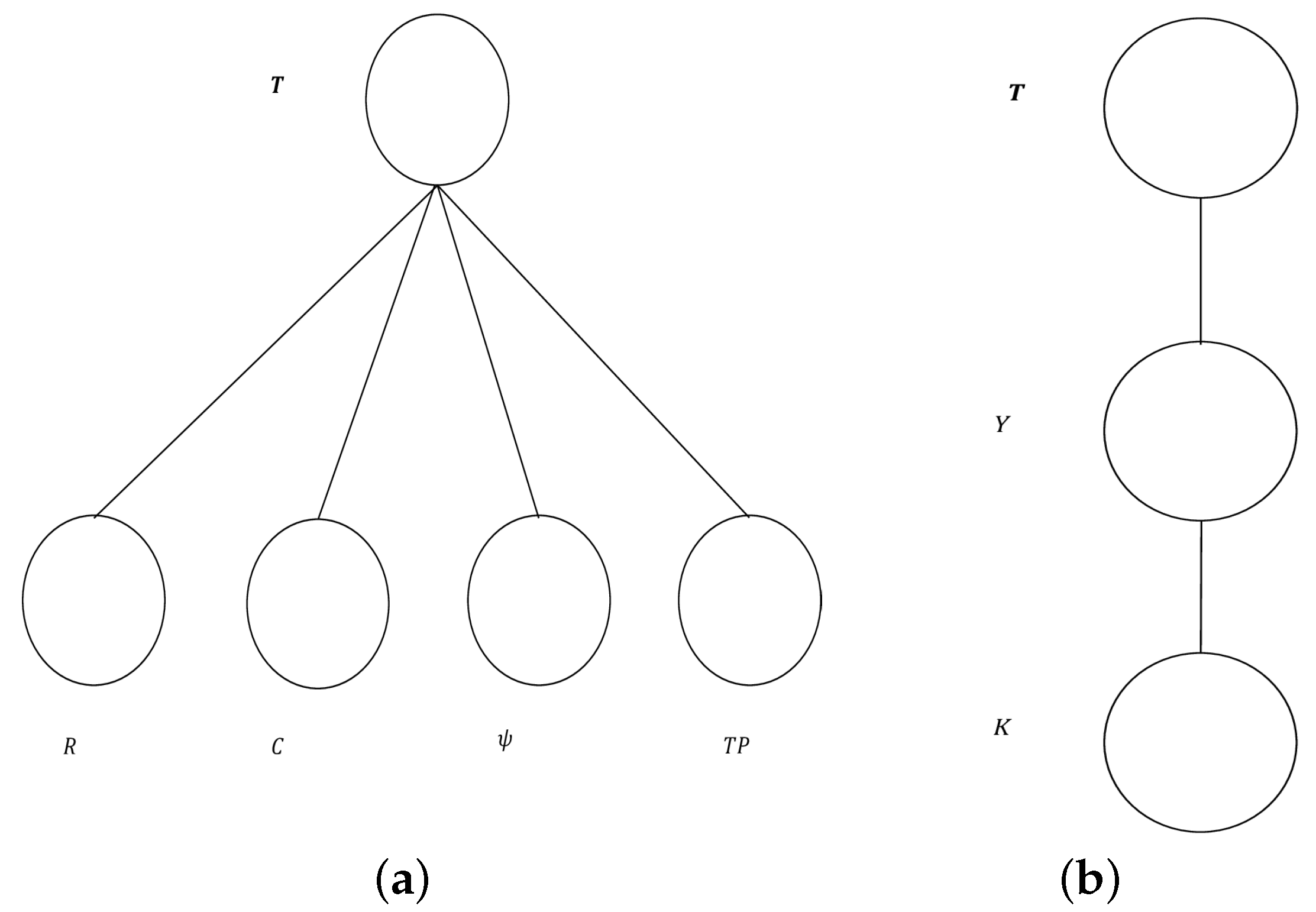
2.4. Model of Water Tributaries with a Tree Structure

Because the region of the water tributaries with a tree structure is homogeneous, its coherent matrix satisfies T W Σ , L , p . Given a tree tributary ψ , if it consists of n single branches C 1 , C 2 , , C n that denote the node of the tree, the structure relationship T P formed by the branches is α 1 , β k , α k , β l , , α l , β n . Both α i and β i are the index of branch C i ; α k , β l denotes the edge of the tree such that α k is the father node and β l is the child node. Then we have
ψ = n , C 1 , C 2 , , C n , T P .
Supposing that ψ satisfies the hypothesis of a Markov field that the label of a single node is only determined by the labels of the adjacent parent and children nodes, then p ψ obeys the Gibbs distribution according to the Hammersley Clifford theorem [28]:
p ψ = 1 Z c C ψ φ X c exp c C ψ E X c ,
where C ψ is the set of a series of cliques in graph ψ , and Z is the normalization constant.
From (7), we get the prior probability of ψ
p ψ exp λ ψ n i = 1 n E C i α i E C i , C β i ,
where E C i denotes the energy of branch C i , E C i , C β i denotes the energy of the branch pair C i and C β i , and α i E C i , C β i denotes the total energy of all branches adjacent to C i ; λ ψ n is the regularization term related to the number of branches.
According to (3), (4) and (8), if the number of regions R r is N r , the number of single branches is N c , and the number of trees is N ψ , the prior probability of image R is
p Θ = i = 1 N r p R i j = 1 N c p C j k = 1 N ψ p ψ k .
Because a free single branch can be considered as a special tree with one node, if the total number of trees including single branches and branches in tree structures is M, the likelihood probability is
p T | Θ = i = 1 N r x , y R r i f T i x , y | Σ i , L , p j = 1 M x , y R c j f T j x , y | Σ j , L , p ,
where T i x , y denotes the coherent matrix of point x , y .
Based on the prior and likelihood probability Formulas (9) and (10) as well as the prior model Formulas (3), (4) and (8), we get the final general model of the segmentation from (1).

3. The Proposed Method

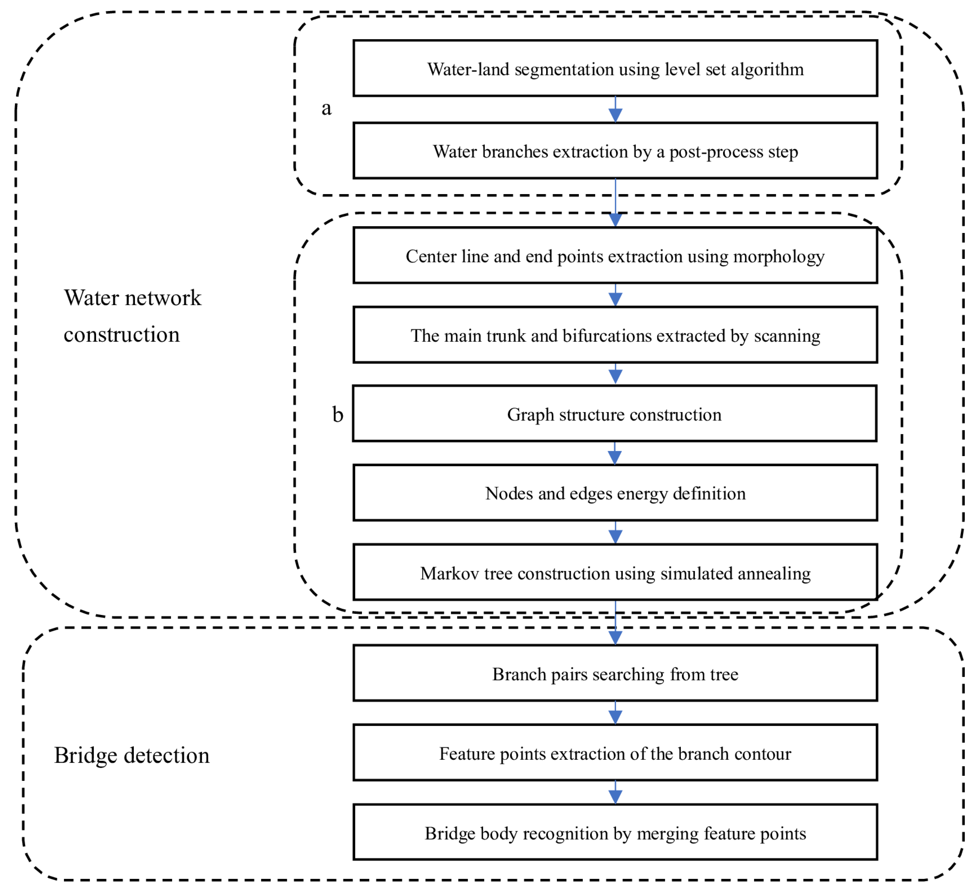
3.1. Overview of the Proposed Method

The optimum parameter Θ can be searched using the Markov Monte Carlo method based on (1). However, the complexity of the algorithm is very high because the parameter space is huge. To reduce the complexity of the general model, a hierarchical model is proposed to divide the model into two layers: one is water branch extraction by segmentation, and the other is a water network connection, as shown in Figure 2b. The general model of the segmentation presented in Section 2 can be represented in Figure 2a, where the latent random variables R , C , ψ , T P denote the four parameters of the model R r , R c , R ψ , T P , and variable T denotes the observed coherent matrices. The hierarchical model is shown in Figure 2b, where the latent variable K denotes whether the water branches belong to the water network, and the latent variable Y denotes whether the segmented regions belong to the land or the water. The hierarchical model can be greedily solved layer by layer based on each graph.
The flowchart of the proposed method is shown in Figure 3. The first part of the algorithm performs the water network construction. The first step of this part performs the water branch extraction, which corresponds to the first layer of the hierarchical model. The second step performs the water branch connection, which corresponds to the second layer of the hierarchical model. The second part of the algorithm performs the bridge detection and bridge body extraction.
The first part of the algorithm is described in Section 3.2 and Section 3.3. The steps of the water branch extraction are shown in box a, where the water and land are segmented using a level set method, and all water branches are extracted by a post-process of the segmentation result. The steps of the water branch connection are shown in box b, where the branches are scanned, tracked, and connected recursively to construct the water network. First, the centerline, endpoints, and directions of each branch are extracted by a morphological processing in a combination of the spline interpolation. Next, the main water trunk and its bifurcations are extracted from the branches using a binary image scanning method. Then, the initial graph structure of a local tributary takes a bifurcation as a root is constructed by connecting branches based on the distance and direction angle of different centerlines. The initial whole graph structure of the water is constructed by connecting different local tributaries. Finally, by defining the node and edge energy of the graph, the optimal Markov tree can be dynamically solved using the simulated annealing algorithm.
The second part of the algorithm is described in Section 3.4. In this part, the adjacent branch pairs for the bridge detection are extracted by traversing the edges of the tree first. The feature points of each branch contour are then extracted using a curve polygon approximation algorithm. Finally, merging the feature points on the contours of the branch pair by distance, the bridge body is extracted to finish the bridge detection.

3.2. Water Branch Extraction

If curve Γ denotes the boundary of the water and land segmentation, then the objective of the two-region segmentation is as follows according to (1):
Γ * = Γ Ω a r g m a x log p T | Γ p Γ ,
where p T | Γ denotes the probability of each region given the segmentation Γ , and p Γ denotes the prior probability of Γ .
According to (3), (10) and (11), the objective energy function of the segmentation can be represented as
E Γ = γ r D R 1 ρ + λ r Γ R 1 log f T 1 x , y | R 1 d x d y R 2 log f T 2 x , y | R 2 d x d y ,
where R 1 is the region inside the curve Γ , R 2 is the region outside the curve Γ , and f T i x , y | R i is the probability distribution function of region R i i 1 , 2 .
If the curve Γ is implicitly embedded into a level set function Φ , the optimal segmentation can be solved by iteratively evolving Φ as the derivative of the energy function to Φ  [29]. When the segmentation is finished, the water and land regions can be identified by comparing the average scattering total power of the two segmented regions. After the final binary result of the land and water segmentation B is obtained, all water branches D = d j j 1 , , N d ( N d denotes the number of branches) can be extracted by determining all connection regions from the water segmentation result.

3.3. Water Branch Connection

If W denotes the water network, the class labels of the branches D are K = k j j 0 , 1 , where k j = 1 means that d j belongs to W , and the value space of W is W , then the general connection model is
K * = K W a r g m a x log p D | K p K .
According to (9), the prior probability of labels K is
p K = i = 1 N c p C i j = 1 N ψ p ψ j ,
where D is composed of several single water branches C i i 1 , , N c and water tributaries with tree structure ψ j j 1 , , N ψ .
Because a single water branch can be considered as a water tributary with a tree structure only containing a root node, formula (14) is equivalent to
p K = i = 1 M p ψ i exp i = 1 M E K i ,
where M is the sum of N c and N ψ ; K i is the label vector of tributary ψ i ; and E K i is the prior energy of tributary ψ i , which can be computed from Formula (8).
According to (10), the likelihood probability model of labels K is
p D | K = i = 1 M f T i D i | ψ i exp i = 1 M E D i | K i ,
where f T i D i | ψ i denotes the likelihood probability of the average coherent matrix T i D i of region D i in case of tributary ψ i , and E D i | K i is the likelihood energy of the tributary  ψ i .
Similarly, joining (15) and (16), the objective energy function of water connection can be represented as
K * = K W a r g m i n i = 1 M E K i + E D i | K i .
To construct the whole water network of the branch set D based on (17), we need to get the geometric representation of the branches first. We then construct the initial graph structure of the branches based on the spatial adjacent relationship of different branches. Finally, we can search the optimal graph structure by defining the prior and connection energy of the branch and solving the connection probabilistic graph model.

3.3.1. Geometric Representation of a Branch

From Section 2.3, we know that to represent a branch, the centerline and its endpoints and directions need to be obtained first. It is difficult to extract the centerline because the shape of branch is varied and some branches are winding. To get a reasonable centerline, we first extract the raw skeleton of the branch using morphological processing and then fit the skeleton into a curve using the spline interpolation. If the extracted centerline of a branch is c m s = x m s , y m s , and s 0 , S , the two endpoints of the branch are c m 0 and c m S , and the two directions of the branch are the tangent directions of points c m 0 and c m S .

3.3.2. Main Trunk and Bifurcations Extraction

The whole water feature is composed of a trunk, several tributaries, and some isolated branches. If the extracted branches set is D = d j j 1 , , N d , where N d denotes the number of branches, the branch with the maximum area d m is selected as the main trunk of the water. There are several bifurcations in the main truck, each of which forms the starting point of a tributary. To determine the adjacent relationship of branches on a tributary, the bifurcations need to be extracted first. The bifurcations are areas protruding from the trunk, flanked by land. Taking a pixel on a bifurcation as the center, the pixels with a certain distance along the two sides of the horizontal or vertical direction are on the land. Thus, we can get the bifurcation by a scanning method. An example segmentation result is shown in Figure 4a, where the region in white is water and the region in black is land. One bifurcation of the main trunk is shown in Figure 4b. We find that the bifurcation is a long strip with land on both sides. Because the direction of the bifurcation is varied, the scanning is carried out in multiple directions at the same time. In this paper, we scanned in two group orthogonal directions, where one group is horizontal and vertical, and the other group is 45 degrees and 135 degrees counterclockwise. As shown in Figure 4b, for pixel P on a bifurcation, the scanning is carried out in four directions. For scanning along the direction τ , if there are land pixels in the range from positive δ r a d to negative δ r a d with P as the center; P is considered as a point in the bifurcation branch. If P is scanned as a bifurcation pixel in the two orthogonal directions, P is classified as a bifurcation pixel in the group directions. If P is classified as a bifurcation pixel in one of the two groups, P is finally classified as a bifurcation pixel.
Because the coastal terrain is uneven, some convex regions are wrongly scanned as bifurcations. To reduce the false regions, the scanned bifurcations are identified by the ratio of length to width, area, and the consistency of width. If the perimeter of a region is l P and the area is A, the ratio of length to width l L / l W can be represented as follows:
ρ L W = l L l W = l P + l P 2 16 A l P l P 2 16 A .
There are some bifurcations with large width and area. As shown in Figure 4a, the tributary marked in the red box is broken into two parts by a bridge. The tributary cannot be extracted as a bifurcation using the scanning method. For this kind of tributary, if a branch in the tributary satisfies that the distance between the contour of the branch and the main water is less than δ r e f and its area is greater than Δ r e f , then it is classified as a bifurcation.

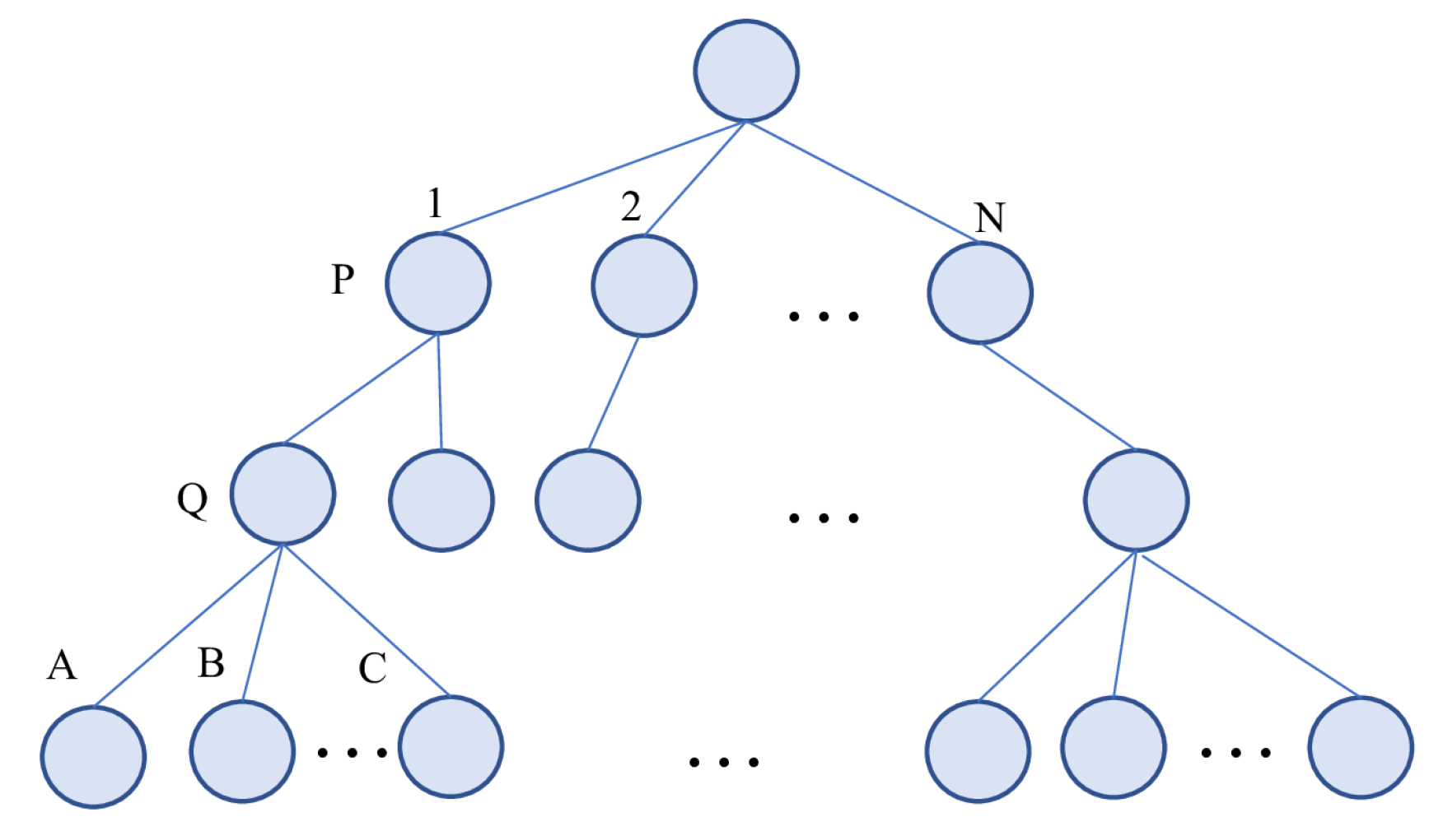
3.3.3. Graph Structure Construction

The N-tree is used to represent the graphical structure of a water tributary. As shown in Figure 5, each node X i in the N-tree denotes a water branch d i . A single node contains one parent node and j j N children nodes. Taking a bifurcation as the root node, a tree is constructed by searching for children nodes according to the distance and direction angle between the centerlines of two branches.
For the branch set D , if d m denotes the extracted main trunk, and H = h x x 1 , , N h denotes the extracted bifurcations on d m , the graph structure of the water network can be recursively built based on the construction algorithm of the tree. First, the angle and distance between each two branches in D are calculated. We take d m as the root node. Using a flag set to mark whether the branches have been built, all branches are initially marked as 0 except branch d m . Then, starting with bifurcation h x , the successor nodes of N-tree are searched in distance limitation δ r e f and direction limitation θ r e f . The children nodes are set to root nodes and the successor nodes are iteratively searched until the leaf node is reached. We mark all the nodes in the N-tree that have been built. Finally, by following the same steps, each sub-tree of the root node d m is successively constructed by starting with a bifurcation that is not searched.

3.3.4. Node and Edge Energy Definition

To construct the graph of branches using the probability model, the prior energy of the branch and the connection energy of two adjacent branches need to be defined according to (8) and (15). As a branch is represented as a node and the connection of two branches is represented as an edge, the prior energy of a branch is called node energy E n o d e , and the connection energy is called edge energy E e d g e .
The expression of the node energy of a branch E n o d e is defined in (5). The values of the area D C and length S are easy to calculate based on the geometric representation of the branch. However, the consistency function of a branch E o w needs to be defined. Given branch d j , if c i s denotes the centerline curve of d j , the left boundary is c l s and right boundary is c r s , then the width function w s is equal to c r s c l s . Because w s may gradually increase or decrease as s for a water branch, E o w is defined as the average of the local width consistency of each point on the centerline. The local width consistency of a point is defined as the difference between its width and the average width of the point in a window region. The average width of each point is calculated using a sliding window. If the average width function is w o s , the width consistency of the branch is defined as follows:
E o w = 1 c i s s w o s w s 2 1 / 2 ,
where c i s denotes the length of c i s .
The edge energy of two adjacent branches is determined by the distance and direction angle of the branches. Supposing that the distance between node Q and node P is δ P Q and the angle of direction is θ P Q , the energy of the edge P Q can be defined as
E e d g e P Q = ε s i n θ P Q + η δ P Q E r e f ,
where the term ε s i n θ P Q restricts the angle of two connected branches; η δ P Q restricts the distance of two connected branches; E r e f is the reference edge energy; and E r e f is subtracted in E e d g e is a mean normalization process so as to keep a balance between the energy of E e d g e and the energy of E n o d e . If the reference angle is θ r e f and the reference distance is δ r e f , E r e f is ε s i n θ r e f + η δ r e f .

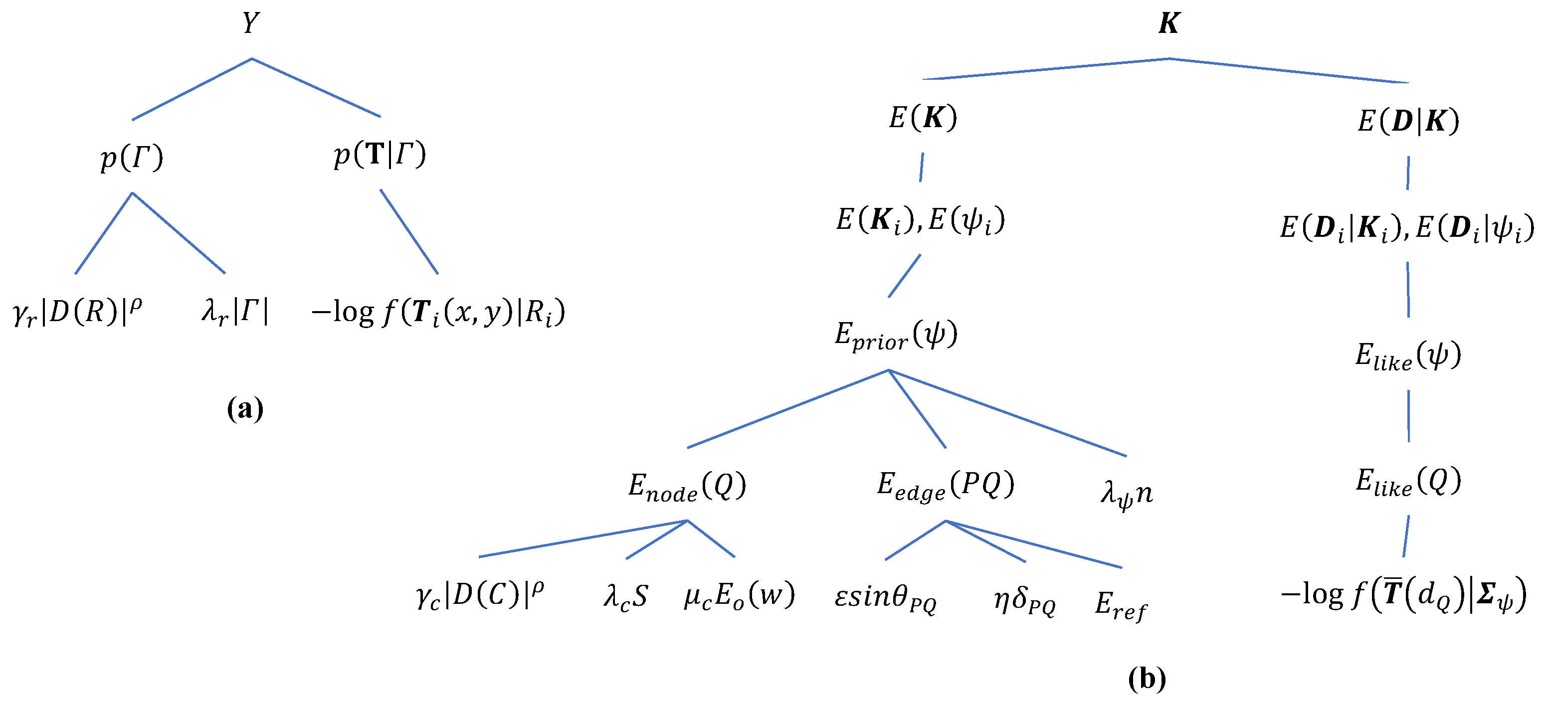
3.3.5. Markov Tree Construction

To construct the tree using (17), the prior and likelihood energies of the whole tree need to be defined.
(1)
Prior energy of Markov tree
From the N-tree structure, we see that the clique of a N-tree ψ is composed of a node, a parent node, and several children nodes adjacent to the node.
As shown in Figure 5, given node Q, if the father node is P and there are j j N children nodes, then the prior energy of Q is the sum of node energy and all edge energies related to Q, and the expression is as follows:
E p r i o r Q = E n o d e Q + 1 2 E e d g e P Q + i O E e d g e Q i
where O is the children nodes set of Q. Because edge P Q is the common edge of two nodes Q and P, the edge energy is only set to half for Q.
Calculating the energy of each node respectively and according to (8), the total energy of N-tree ψ is
E p r i o r ψ = λ ψ n + Q ψ E p r i o r Q ,
where n is the number of nodes.
(2)
Likelihood energy of Markov tree
Given node Q, if it belongs to tree ψ , the likelihood energy is determined by the average coherent matrix Σ ψ of region ψ :
E l i k e Q = E d Q | k Q = log f T ¯ d Q | Σ ψ ,
where k Q is the class label of Q; d Q denotes the region of branch Q; and T ¯ d Q is the average coherent matrix of d Q .
Similarly, the total likelihood energy of N-tree is the sum of the likelihood energy of each node:
E l i k e ψ = Q ψ E l i k e Q .
The structure diagram of the symbols defined in the model of the water network construction from Section 2, Section 3.2 and Section 3.3 is shown in Appendix B.
(3)
Network construction based on Markov tree in global searching
According to (22) and (24), the energy of the whole water network (17) can be obtained. The optimum solution of labels K can be solved by searching the minimum of the objective energy function in space W using the Monte Carlo method or the simulated annealing method [30].
If we add the rate parameter ξ in a Gibbs distribution, i.e., p K exp ξ E K , the steps of the simulated annealing algorithm (Algorithm 1) are as follows.   
Algorithm 1: Water network construction based on Markov tree in global searching.
Step 1:
Initialization. Initialize the label vector of water network branches to K 0 randomly. Set the limited angle of branches to θ r e f and the limited distance to δ r e f . Set the maximum number of the children nodes of tree to N, the initial parameter ξ , the learning rate l r , the step size of parameter update N u p , and the maximum number of iterations N m a x .
Step 2:
Build the network graph model. For branches with label 1 in K i , the angle and distance between each two branches are calculated first. Take the branch with the maximum area as the root node. The successor nodes of the N-tree are then searched in distance limitation δ r e f and direction limitation θ r e f . The children nodes are set to root nodes, and the successor nodes are iteratively searched until the leaf node is reached. Mark all the nodes in the N-tree that have been searched. Following the same steps, the unmarked node with the maximum area is set as the new root node to search a new tree until all the branches with label 1 are marked. After all the sub-trees ψ i have been searched, the total energy of the network E i K is calculated using ψ i .
Step 3:
Update the state variables. Flip the label k j of branch d j randomly to update K i to K i + 1 . Build the network graph again according to step 2 and update the energy of network to E i + 1 K . Accept the change of label k j according the following probability:
a ξ = m i n 1 , exp ξ E i + 1 K E i K .
Step 4:
Update parameter ξ . Repeat step 3 until the maximum number of iterations is reached, where ξ is updated to ξ l r every N u p iterations.
(4)
Network construction based on Markov tree in local searching
Because the water network is complex, as the number of branches is large and the sizes of different branches are varied, global searching is difficult to converge to the optimal value. For SAR images, the area of some tributaries is very small, and the contours are uneven due to speckle noise. It is easy to ignore the branches with weak energy if the global searching algorithm is used. However, an important feature of the N-tree is that the global optimum must be the local optimum. According to (21) and (24), the energy of an N-tree can be decomposed into the energy of the root node, adding all the energies of the sub-tree, taking each child node as root. Thus, the global optimum can be dynamically searched locally. If H = h x denotes the extracted bifurcations of the main trunk, the water network construction algorithm based on local iterative searching (Algorithm 2) can be described as follows.
Algorithm 2: Water network construction based on Markov tree in local searching.
Step 1:
Extract the main trunk and bifurcations. The branch with the maximum area d m from the branch set D = d j j 1 , , N d is selected as the main water. Extract the main trunk and bifurcations H = h x using the scanning method in a scanning radius δ r a d .
Step 2:
Build the network graph of a tributary. Take d m as the root node and start with bifurcation h x in H to build a tree. Calculate the angle and distance between h x and others branches d j j m . Search the children nodes of h x in the tree under the limitation of θ r e f and δ r e f . Then, take each child node as the root node to search its children nodes until the leaf node is reached to get the current sub-tree ψ x .
Step 3:
Search the Markov tree using simulated annealing. Take ψ x as a water network and search the optimal tree using simulated annealing similar to Algorithm 1.
Step 4:
Iteration. Repeat steps 2 and 3 until all elements in H complete the tree construction.

3.4. Bridge Detection and Bridge Body Extraction

When the final water network is obtained, all the adjacent branch pairs can be easily extracted by determining all edges of the network using the depth traversal algorithm of the tree because each edge denotes an adjacent branch pair. For an extracted branch pair, if the ROI of the bridge is directly extracted by merging the points on the two contours by distance, some boundary points that are not on the bridge will be wrongly classified to the ROI of bridges when the branch is narrow enough. As shown in Figure 6a, two narrow branches are adjacent to each other, where the region in gray is the land. The region marked by the black rectangle box is the ROI extracted by distance merging. We find that part of the boundary on the land is wrongly extracted.
Because the angle between a bridge and the surrounding land is nearly 90 degrees, the junction between the bridge and the water contour is distinct. To avoid the wrong extraction, the ROI of a bridge is extracted by merging the distinct points extracted from the water contour.
The feature points of the water contour are extracted using the Douglas–Peucker (DP) splitting and merging algorithm [31]. The DP algorithm recursively splits a curve to two segments at the middle point of the curve until the distance between each point on the curve and the straight line linking two adjacent feature points is less than a distance tolerance δ t o l . Given two adjacent branches shown in Figure 6b, if the set of feature points of branch 1 is P 1 and branch 2 is P 2 , the feature point pairs in close distance can be extracted under the threshold of the reference distance δ r e f . The feature points on the boundary can then be obtained by the spatial coordinate relationship. If the feature points of branch 1 are o 11 , o 12 and branch 2 are o 21 , o 22 , the pixels on the land inside the quadrilateral surrounded by points o 11 , o 12 , o 21 , o 22 are recognized as the bridge body. Sometimes only one feature point can be detected in branch 1 or 2, so the bridge body can be recognized as follows.
In the case of o 11 = o 12 and o 21 = o 22 , the segment linking o 11 to o 21 is recognized as the bridge body.
In the case of o 11 o 12 and o 21 = o 22 , given a land pixel s in the quadrilateral, if o 11 o 12 × o 11 s · o 11 s × o 11 o 21 > 0 , o 12 o 21 × o 12 s · o 12 s × o 12 o 11 > 0 and o 21 o 11 × o 21 s · o 21 s × o 21 o 12 > 0 , then s is inside the triangle o 11 o 12 o 21 and is recognized as a pixel on the bridge body, where “×” denotes the vector cross product, “·” denotes the vector dot product, and if a = a x , a y , b = b x , b y then a × b = a x b y a y b x .
In the case of o 11 = o 12 and o 21 o 22 , the rule is the same as the case of o 11 o 12 and o 21 = o 22 .
In the case of o 11 o 12 and o 21 o 22 , given a land pixel s in the quadrilateral, if o 11 o 12 × o 11 s · o 11 s × o 11 o 22 > 0 , o 12 o 21 × o 12 s · o 12 s × o 12 o 11 > 0 , o 21 o 22 × o 21 s · o 21 s × o 21 o 12 > 0 , and o 22 o 11 × o 22 s · o 22 s × o 22 o 21 > 0 , then s is inside the quadrilateral o 11 o 12 o 21 o 22 and is recognized as a pixel on the bridge body.

4. Experimental Results and Analysis

Three quad-polarization SAR data acquired by RADARSAT-2 and TerraSAR-X sensors are used to test the proposed algorithm. The ground truth (GT) was drawn with reference to the Google earth map. The algorithm parameters were obtained by making statistics of true bridges and water branches first. Five experiments were then carried out to evaluate the performance of the proposed algorithm. In the first experiment, data over part of Singapore region was tested to show the detailed process flow of the proposed method. In the second experiment, the proposed method was tested for different sites. In the third experiment, the proposed method was compared with the method that constructed the water network by merging water branches by contour distance [32]. In the fourth experiment, the performance of the proposed method using quad-polarization SAR images was compared with that of three different single-polarization channel data. Finally, the bridge body recognition performance of the proposed method was compared with that of the traditional method based on spatial relationships [3]. In all the tests, the performance of the bridge detection was evaluated using detection rate and false rate. The performance of the bridge body recognition was evaluated using the intersection over union (IoU) index.

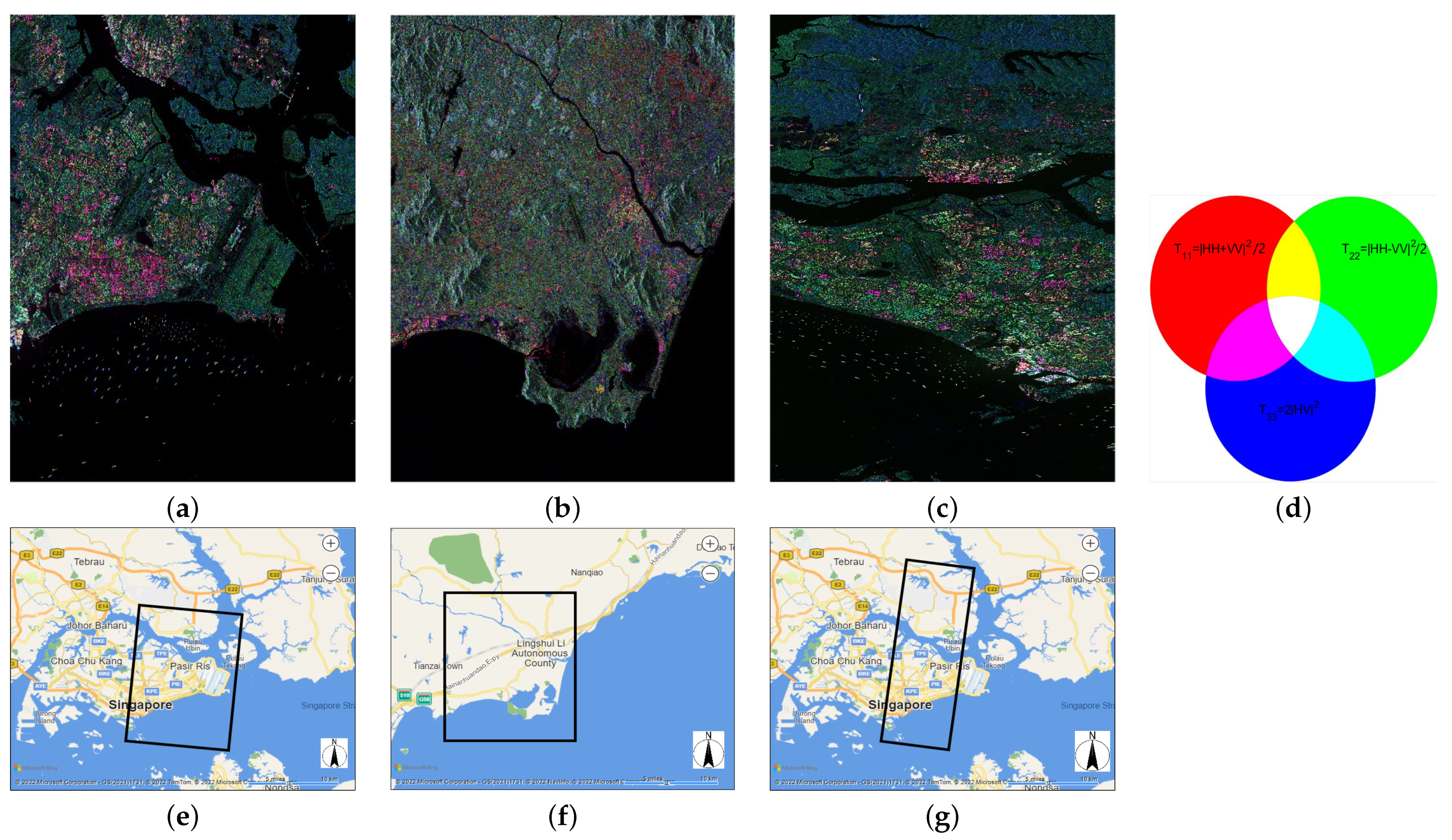
4.1. Data Description

Single look quad-polarization SAR data acquired by RADARSAT-2 sensor over the Singapore region in 2013 and the Lingshui, Hainan province, China region in 2014 and Multi-look quad-polarization SAR data acquired by TerraSAR-X sensor over the Singapore region in 2014 are used to test the proposed algorithm. When the proposed method is carried out, the coherent matrix (directly transformed by the Sinclair matrix for single look data) is calculated as the input data. The details of the data are listed in Table 1. The size of image is 6161 × 4256 for the Singapore image from RADARSAT-2, 5937 × 3920 for the Lingshui image, and 5500 × 2500 for the Singapore image from TerraSAR-X. The corresponding resolutions are 4.73 m × 4.80 m, 4.73 m × 5.47 m, and 2.06 m × 6.59 m, respectively. The detailed parameters of data are listed in Table 1. The Pauli pseudocolor images and geographic legends of the three data are shown in Figure 7, where “R”, “G”, and “B” denote the three components of the Pauli vector. To keep the balance of color contrast, each component is divided by its mean when the image is shown. The data of Singapore from RADARSAT-2 is shown in Figure 7a, the data of Lingshui is shown in Figure 7b, and the data of Singapore from TerraSAR-X is shown in Figure 7c. The color code of the image is shown in Figure 7d. The geographic legends are shown in Figure 7e–g. The topology of the water in Singapore is so complex that it forms a network from Figure 7a,c. The topology of the water in Lingshui is simple, but the tributary is so narrow that the bridges are difficult to detect from Figure 7b. If the main water branch is taken as the root of a tree, the structure of the whole water network is very similar to a tree.

4.2. Parameters Setting

According to Section 3, the parameters of the proposed method include four parts: level set segmentation, the main water scanning, the water network connection, and the bridge bodies recognition. With respect to the water and land segmentation using the level set method, the curve regularization parameter λ r is set to 0.2 and γ r is set to 0.1, as in reference [18]. With respect to the main water scanning, supposing that the input image resolution is R x × R y , the equivalent resolution in x and y directions is R = = R x 2 + R y 2 / 2 . The maximum length of the bridge is L b . The maximum width of the bridge is W b . Then, the equivalent value of L b is L b = L b / R = The equivalent value of W b is W b = W b / R = . With respect to the main water scanning, the scanning radius δ r a d is initially set to W b / 2 . As a scanned bifurcation is also a long strip area, its length is usually far larger than the width, so that the ratio of length to width ρ L W is usually far greater than 2. To avoid missing the scanned bifurcations of some water tributaries, the ratio of length to width ρ L W is set to a small value, 3, according to experimental statistics. Thus, when selecting the broken adjacent branches of the main water, the reference distance δ r e f is set to W b and the reference area Δ r e f to L b × 4 L b .
With respect to the water network connection, when building the graph of the tree structure, the maximum number of children nodes N is set to 2 or 3 and the reference angle to 45 . To set the optimum parameters for the energy calculation of the tree structure, we first extracted 270 water branches by segmenting data 1 in Table 1, as shown in Figure 8. The histogram distribution of three geometric parameters, including length l L , area, and the defined width consistency E o w , of the 270 water branches were then computed through statistics, as shown in Figure 9, where the area is processed by quadratic square root. Statistics results show that the median of the length is 28.0, the area is 19.6, and the width consistency is 0.68. We observe that the histograms of length and area are concentrated, but the histogram of consistency is scattered from Figure 9. When calculating the energy of the tree structure, to keep a balance among the three parts of energies, the parameter of node energy μ c is set to 10, γ c to 1, ρ to 0.5, and λ c to 1 because the counted median of the length and the square root area is about 10 times the width consistency. To keep a balance between the edge energy related to distance and the edge energy related to direction, parameter ε is set to 50 and η to 1 because the average distance between two adjacent branches is almost 50 times to the average sine of the angle. When calculating the total energy, λ ψ is set to 1. When the simulated annealing algorithm is carried out, the initial parameter ξ is set to 0.05, the learning rate l r is set to 1.1, the updating step parameter N u p is set to 50, and the maximum number of iterations N m a x is set to 1000, according to experimental statistics.
With respect to bridge bodies extraction, the distance tolerance for the extraction of feature points δ t o l is set to 0.1 L b 2 + W b 2 to ensure the endpoint junction of the bridge is correctly extracted. The distance tolerance for the merging of feature points is also set to δ r e f .

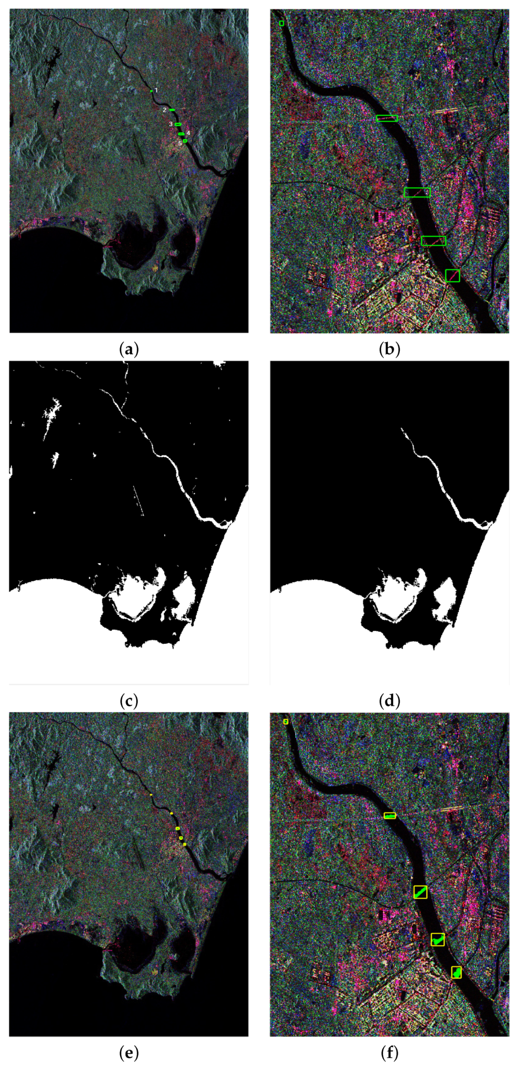
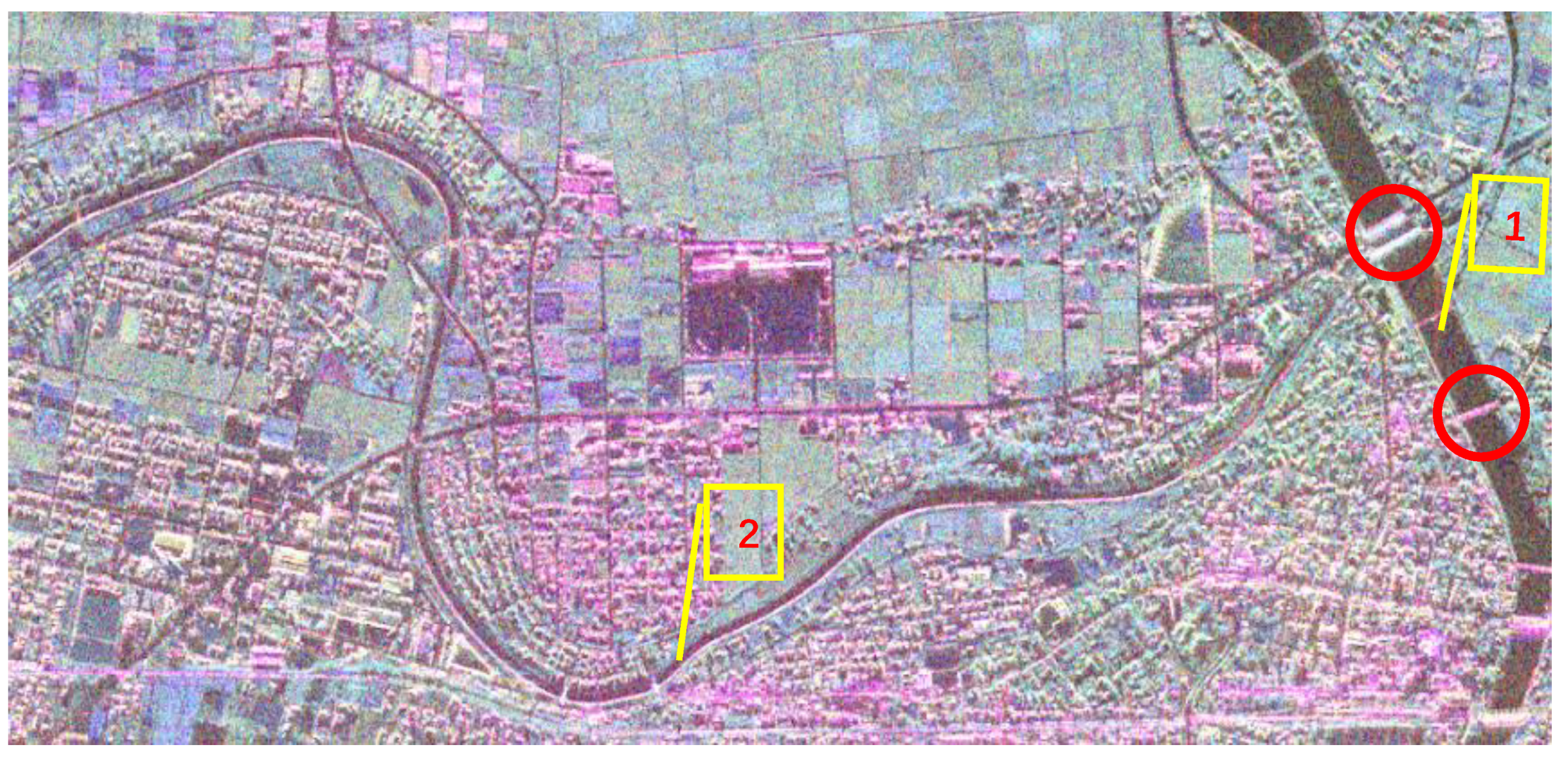
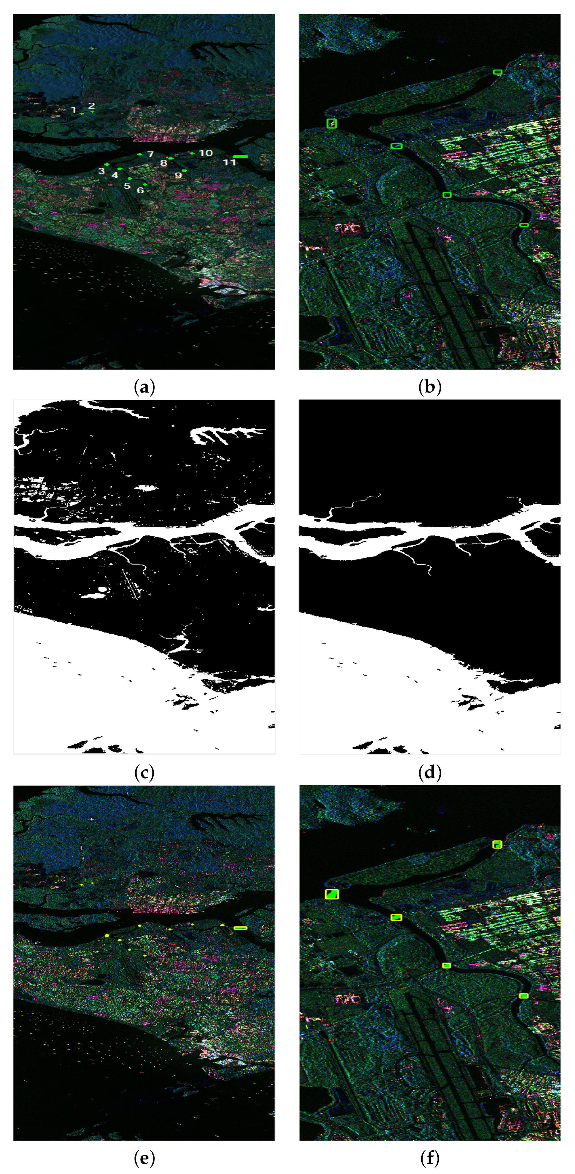
4.3. Example Results

An image covering part of the Singapore region obtained by a 4 × 4 multi-look processing of data 1 is tested to show the algorithm flow of the proposed method. The size of the image is 1000 × 1000 . The Pauli pseudocolor image is shown in Figure 10a. From Figure 10a, we find that the coastal topography of the data is complex. Bridges are distributed in various tributaries with different shapes. There is a large sea-crossing bridge and some small bridges over narrow tributaries. It is difficult to segment and connect the branches on the narrow tributaries. The result of water and land segmentation using level set is shown in Figure 10b. The observation result shows that water and land are correctly separated, but some low scattering regions in the land are wrongly classified as water regions. The extracted main water is shown in Figure 10c. The branches other than the main water are shown in Figure 10d. We observe that there are some tributaries in the main water from Figure 10c. The shapes of tributaries are varied, and some of them are so narrow that the branches on the tributary cannot be connected from Figure 10d. The bifurcation scanning results of the main water is shown in Figure 10e, where the regions in gray marked in the red box are the scanned bifurcations. The observation result shows that the bifurcations of the main water are well scanned by the orthogonal direction scanning method. The final connection result of the water network is shown in Figure 10f. We find that all tributaries are correctly extracted and some small branches on the tributaries are also correctly connected. The results of bridge detection and bridge body extraction are shown in Figure 10g, where the detected bridge bodies are marked in red. The corresponding regions of the detected bridges in the original image are shown in Figure 10h, where the detected bridges are marked by yellow boxes and the bridge bodies are drawn in green. We find that most of the bridges are correctly detected and the corresponding bridge bodies are also accurately extracted.

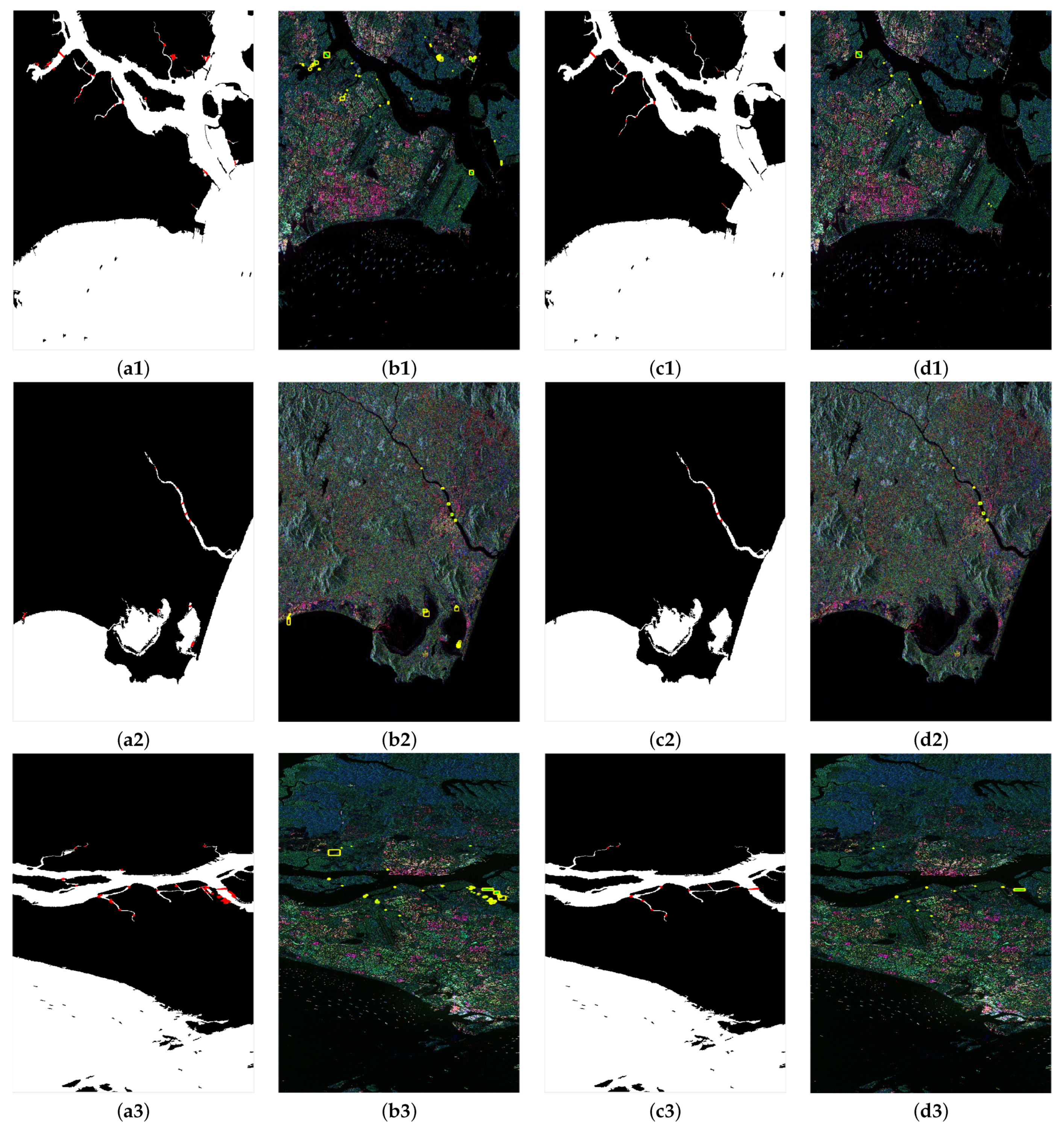
4.4. Performance Evaluation of the Proposed Method under Different Sites

To validate the robustness of the proposed method, the method was tested for different sites using the three testing datasets listed in Table 1. The results of data 1, data 2, and data 3 are shown in Figure 11, Figure 12 and Figure 13, respectively. The ground truth of the bridges is shown in Figure 11a, Figure 12a and Figure 13a, where the bridges are marked by green boxes. Different bridges are located on different branches in Figure 11a, Figure 12a and Figure 13a. An enlarged view of part of the image near a narrow tributary is presented in Figure 11b, Figure 12b and Figure 13b. Some bridges are too small to be clearly observed from Figure 11b, Figure 12b and Figure 13b. The water branch extraction result is shown in Figure 11c, Figure 12c and Figure 13c. There are so many branches of different sizes that they are difficult to connect. The water branch connection result is shown in Figure 11d, Figure 12d and Figure 13d. We observe that the water network is well constructed, and even some small branches on the narrow tributaries are correctly connected in Figure 11d, Figure 12d and Figure 13d. The results of bridge detection and bridge body extraction are shown in Figure 11e, Figure 12e and Figure 13e, where the detected bridges are marked by yellow boxes and the bridge bodies are drawn in green. The detection results of the enlarged part of Figure 11e, Figure 12e and Figure 13e corresponding to Figure 11b, Figure 12b and Figure 13b are shown in Figure 11f, Figure 12f and Figure 13f. Comparing Figure 11b, Figure 12b and Figure 13b with Figure 11f, Figure 12f and Figure 13f, we find that almost all the small bridges over the narrow tributary are correctly detected.
According to the ground truth, the detection performance of the three datasets are listed in Table 2. For data 1, 13 of the 16 bridges are correctly detected and only 1 false alarm target is detected. The detection rate is 81.3%, and the false alarm rate is 7.14%. For data 2, all 5 bridges are correctly detected, and the number of false alarm targets is 0. The detection rate is 100%, and the false alarm rate is 0. For data 3, 10 of the 11 bridges are correctly detected, and only 1 false alarm target is detected. The detection rate is 90.9%, and the false alarm rate is 9.09%.

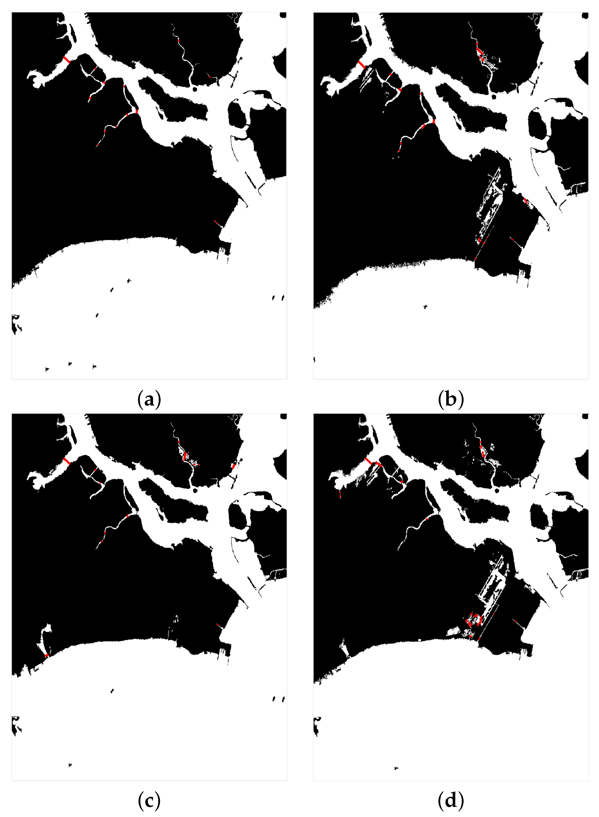
4.5. Comparison of the Proposed Method with Branch Merging Method

In the third experiment, the performance of the proposed method was compared with the one that constructs a water network by merging water branches by contour distance [32] (branch merging method). The comparison results are shown in Figure 14. The comparison results of the three testing datasets are shown in the three lines of Figure 14, respectively. Figure 14a1–a3,b1–b3 are results of the comparison method. Figure 14c1–c3,d1–d3 are results of the proposed method. Figure 14a1–a3,c1–c3 are results of the water network construction, where the detected bridge bodies are marked in red. Figure 14b1–b3,d1–d3 are results of the bridge detection, where the bridges are marked by yellow boxes and the bridge bodies are drawn in green. Compared with Figure 14a1–a3,c1–c3 as well as Figure 14b1–b3,d1–d3, the result of the proposed method is significantly better. The detection performance of the comparison method is listed in Table 3. For data 1, 12 bridges are correctly detected but with a higher number of false alarm targets, at 68. The detection rate is 75%, but the false alarm rate is 85%. For data 2, all bridges are also correctly detected by the comparison method but with a higher number of false alarm targets, at 16. The detection rate is 100%, but the false alarm rate is 76.2%. For data 3, 10 bridges are correctly detected but with a higher number of false alarm targets, at 57. The detection rate is 90.9%, but the false alarm rate is 85%. Compared with the proposed method listed in Table 2, the number of correctly detected targets of the proposed method is larger, while the number of false alarms is greatly reduced.

4.6. Comparison of Quad-Polarization with Single-Polarization Data

To evaluate the gains of polarization data, the performance of quad-polarization data is compared with that of three different single-polarization channels. Compared with quad-polarization data, all the algorithm steps and parameters of the single-polarization data are the same except replacing the coherent matrix with intensity for the computation of likelihood energy. The results of data 1 are shown in Figure 15, where the detected bridges marked in red are shown on the water network result. The result of quad-polarization data is shown in Figure 15a. The results of HH, HV, and VV channels are shown in Figure 15b–d, respectively. We observe that there exist some false alarm targets for the HH and VV channels and some missing targets for the HV channel. As the procedures of water network construction and bridge body recognition are almost the same for the two kinds of data, the cause for that is the difference of the water–land segmentation results. For HH and VV channels, some low intensity regions along the ocean are wrongly recognized as bridge. That is because the low intensity regions connecting different small water regions inside the land are wrongly segmented, and then the area and direction of the water branch are changed. For the HV channel, the cause for error is that some pixels on the bridge are wrongly segmented as water, causing the bridge regions to be broken, and the two adjacent branches are then directly connected. The detection performance is listed in Table 4. The detection rate of the quad-polarization data is 81.3 % , which is higher than that of the three single-polarization data. The highest detection rate is 62.5 % in the HH channel, and the lowest detection rate is 25.0 % in the VV channel among the three single-polarization channels. The false alarm rate of the quad-polarization data is 7.14 % , which is less than that of the single-polarization data. The lowest false alarm rate is 38.5 % in the HV channel among the three single-polarization channels.

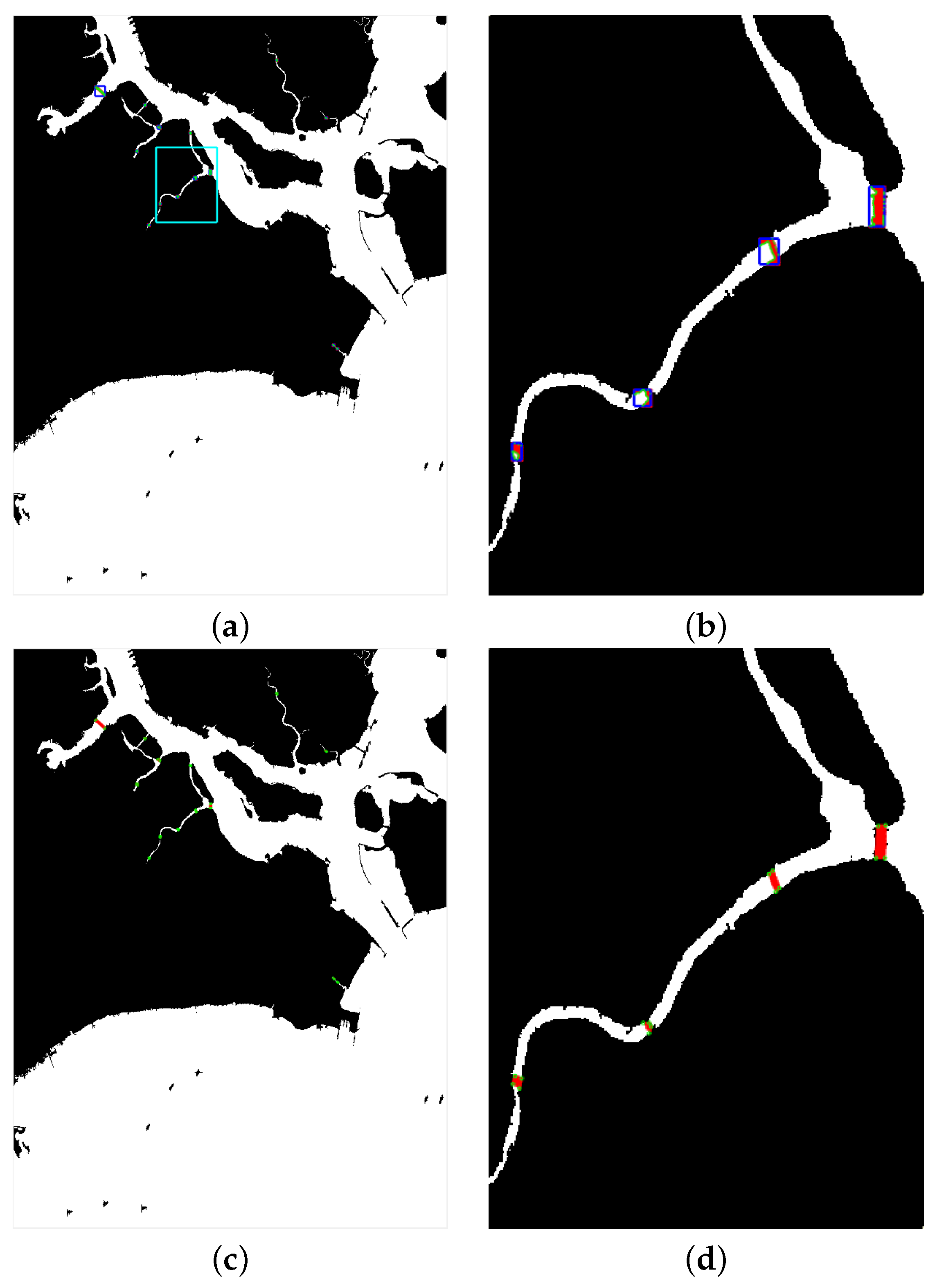
4.7. Comparison of the Bridge Body Recognition between the Proposed Method and the Spatial Method

As the summary described in Section 1, most of the existing bridge detection methods extract bridge bodies by the spatial relationship of bridge with water based on the water segmentation result. However, some boundary points that are not on the bridge will be wrongly classified to the bridge when the water branch is narrow if those spatial methods are used, as shown in Figure 6. In the last experiment, we compared the bridge body recognition performance of the proposed method with that of the traditional method based on spatial relationship (the spatial method). Both methods obtain the water result from the proposed water network construction method. The spatial distance threshold is set to δ r e f , as in Section 3.2, for the spatial method. The results are shown in Figure 16, where the recognized bridge bodies marked in red are all mapped on the water network result. The result of the spatial method is shown in Figure 16a, where the recognized bridge bodies are marked in a blue box, and the extracted contour pixels by spatial relationship are marked in green. The local region marked in cyan in Figure 16a is shown in Figure 16b. We observe that some pixels of the recognized bridge bodies are not on the bridge. The result of the proposed method is shown in Figure 16c, where the extracted feature points are marked in green circles. The result of the same local region as Figure 16b is shown in Figure 16d. We find that all the recognized bridge bodies are accurately located on the bridge. We compute the IoU between the detected box and the ground truth shown in Figure 11a. The mean IoU index of the proposed method is 99.5 % , but the index of the spatial method is only 68.9 % . The performance of the proposed method is much better than that of the spatial method.

5. Discussion

With respect to the offshore bridge detection problem in SAR images, the proposed method introduces a novel solution by constructing the water network using the probability graph model of a Markov tree. The experimental results of two RADARSAT-2 data and one TerraSAR-X datum show that the false alarm rates of the proposed method are less than 10%, and the detection accuracies are larger than 85%.
The difficulties of offshore bridge detection include the extraction and connection of water branches. By defining the internal and external energies of the segmentation curve and embedding the energy into a level set function, all connected branches are accurately extracted by the level set segmentation method. The segmentation results of the three experimental data showed that the extracted water branches were accurate and smooth. Because the number of water branches are large, the structure of the branches is complex, and there are many small and narrow branches, it is difficult to connect the branches merging directly by distance. By building the graph structure of the connection model using the tree structure, the branches are effectively organized because the tree structure is ordered from root to leaf so that each parent branch only has two or three child branches. The observations of the three experimental data showed that the structure of the water of each datum is similar to a tree. By defining the node energy and the edge energy of the tree and searching the extremum of the energy using the simulated annealing algorithm, the global optimum solution of the water branch connection is solved. Experimental results showed that the false alarm rates of the proposed method were greatly reduced compared to the method of merging branches contour by distance. Because the sizes of bridges are varied, there will some boundary points of the land wrongly recognized as the ROI of bridges. By extracting the feature points of the branches and merging them by distance, the bridge bodies are more accurately recognized. Experimental results showed that the mean IoU index of the proposed method was 99.5%, which is much larger than 68.9% of the spatial method.
Although the water connection algorithm is complex, the time-consuming step is mainly in the water and land segmentation. For the segmentation, if the size of the image is n × n , the time complexity is O n 2 . For the bifurcation scanning, if the scanning windows are designed before scanning, the time complexity of the scanning of one pixel is O 1 . Because the size of the image is n × n , the time complexity of the whole scanning is O n 2 . However, it is easy to scan in parallel, so the time complexity of the entire scanning is O 1 . For the graph construction, the time complexity of the tree construction algorithm is O n . For the Markov tree construction, if the number of nodes is n and the number of iterations is m, the complexity of the simulated annealing algorithm is O m n because the time complexity of the tree construction algorithm is O n . Thus, the most time-consuming step is segmentation, and the total time complexity of the proposed algorithm is O n 2 . In the test, the time of each step of the proposed algorithm was calculated. The testing platform was MATLAB v9.5, and the CPU was an Intel Xeon at 3.6 GHz with 16 GB RAM. For data of Singapore in the example test, the time of segmentation is 135.7 s, bifurcation scanning is 0.85 s, graph construction is 2.46 s, and Markov tree construction is 2.78 s.

6. Conclusions

We have proposed a bridge detection method for quad-polarization SAR images, which is based on a water network connection using the Markov tree probability graph model. By establishing the general segmentation model of the whole water network using Bayesian criterion, the bridge detection problem is converted to a two-layer hierarchical model, including the segmentation of land and water and the connection of different water branches. According to the similarity between the structure of water network and a tree, the connection of water branches is converted to the construction of tree by taking each water branch as a node. By defining the energy of the node and edge of the graph, the optimum solution of the tree is recursively searched using a tree-structure simulated annealing algorithm. Because a level set segmentation model and the Markov tree probability graph connection model are used, the extracted water network is accurate and robust to speckle noise and scattering interference. Finally, to avoid wrong results caused by merging contour by distance, bridge bodies are extracted by merging the feature points of the contours of each branch pair of interest. Evaluations of the proposed method as well as comparisons with the bridge detection method of merging water branches by contour distance using three quad-polarization data acquired by RADARSAT-2 and TerraSAR-X show the potential of the proposed method. The detection rate of the proposed method is higher than 85%, and the false alarm rate is lower than 10%. Compared with the branch merging method, the false alarm rate of the proposed method is far less, whereas the detection rate is slightly higher. Compared with the spatial method, the IoU index between the recognized bridge body and ground truth of the proposed method is also much improved. Compared to the three different single-polarization channels of the quad-polarization data, the performance of quad-polarization data is much better because of accurate segmentation.
From the analysis and verification of the experimental results, we find that the proposed method still cannot detect bridges over the tributaries interfered with by strong scatterers. In future work, polarimetric scattering parameters that can reduce the strong scattering interference components in the water area will be extracted to segment water and land. The proportion of error segmented water regions will be effectively decreased by those polarimetric parameters. At the same time, before the water network is connected by the proposed method, we will take a path tracking algorithm, such as particle filter, to track the tributary broken by large distances.

Author Contributions

Conceptualization, C.L. and J.Y.; methodology, C.L.; software, C.L.; validation, C.L., J.O. and D.F.; formal analysis, J.Y.; investigation, J.O.; resources, J.Y.; data curation, D.F.; writing—original draft preparation, C.L.; writing—review and editing, J.Y.; visualization, C.L.; supervision, J.Y.; project administration, C.L.; funding acquisition, C.L. and J.Y. All authors have read and agreed to the published version of the manuscript.

Funding

This work was supported in part by the National Natural Science Foundation of China (NSFC) (No. 62101456 and 62171023), and in part by 2022 Suzhou innovation and entrepreneurship leading talents program (Young innovative leading talents), and in part by the Fundamental Research Funds for the Central Universities (No. D5000210752).

Data Availability Statement

Please contact Chun Liu ([email protected]) for access to the data.

Acknowledgments

The authors would like to thank the reviewers for their valuable comments and suggestions. The data were provided by the laboratory of polarimetric radar and remote sensing applications of Tsinghua University and the China National Satellite Ocean Application Service.

Conflicts of Interest

The authors declare that there is no conflict of interest regarding the publication of this paper.

Appendix A

The nomenclature of all symbols in each section is shown in the following table.
Table A1. The nomenclature of all symbols in each section of the article.
SectionSymbolNomenclature
Section 2.1 R The image plane
T The given polarimetric SAR image
T P The topological relationship
R r Homogeneous regions
R c Free curve branches
R ψ Tree regions
Θ The parameter set R r , R c , R ψ , T P
Ω The parameter space of Θ
p Θ The prior probability of Θ
p T | Θ The conditional likelihood probability of Θ
N r The number of regions R r
N c The number of single branches R c
N ψ The number of trees R ψ
Section 2.2 Σ , Σ j The average coherent matrix
LThe number of looks
T The coherent matrix
pThe number of polarimetric channels
W Σ , L , p The Wishart distribution
f T | Σ , L , p The probability of the coherent matrix T
p R The prior probability of a segmentation region
D R The area of region R
R The contour length of region R
γ r , ρ , λ r The parameters of p R
Section 2.3CA water branch
SThe whole length of the centerline of a branch
D C The region of the branch C
c s The center curve of a branch
w s The width of a branch
p C The prior probability of branch C
p D C The prior probability of region D C
w s The width of a branch
p w s The prior probability of width w s
E C The prior energy of branch C
D C The area of region D C
E o w The consistency function of w s
γ c , ρ , λ c , μ c The parameters of E C
Section 2.4 ψ A tree tributary
p ψ The prior probability of ψ
E C i , C β i The energy of the branch pair C i and C β i
Section 3.2 Γ The boundary of the water and land segmentation
p T | Γ The likelihood probability given the segmentation Γ
p Γ The prior probability of Γ
d j A water branch
D = d j The set of the water branches
N d The number of branches
Section 3.3 W The water network
K The labels of the branches D
W The value space of W
K i The label vector of tree ψ i
p K The prior probability of K
p D | K The likelihood probability of the K
p K i , p ψ i The prior probability of tree ψ i
E K i , E ψ i The prior energy of tree ψ i
E D i | K i , E D i | ψ i The likelihood energy of tree ψ i
Section 3.3.1 c m s The centerline of a branch
c m 0 , c m S The two endpoints of a branch
Section 3.3.2 δ r a d The scanning radius
l P The perimeter of a region
AThe area of a region
ρ L W The ratio of length to width
Section 3.3.3N-treeThe number of children nodes in a tree
δ r e f The reference distance
θ r e f The reference angle
H = h x The extracted bifurcations
N h The number of the bifurcations
Section 3.3.4 E e d g e P Q The edge energy of the edge P Q
E r e f The reference edge energy
Section 3.3.5 E p r i o r Q The prior energy of branch node
E n o d e Q The prior node energy of branch node Q
E p r i o r ψ The prior energy of tree ψ
nThe number of nodes in a tree
λ ψ The parameter of regularization term λ ψ n
E l i k e Q The likelihood energy of branch node Q
E l i k e ψ The likelihood energy of tree ψ

Appendix B

The structure diagram of all symbols used in the water network construction is shown in Figure A1.
Figure A1. Diagram of the symbols in the model of water network construction: (a) diagram of water branch extraction; (b) diagram of water branch connection.
Remotesensing 14 03888 g0a1

References

  1. Lee, J.; Krogager, E.; Ainsworth, T.; Boerner, W. Polarimetric analysis of radar signature of a manmade structure. IEEE Geosci. Remote Sens. Lett. 2006, 3, 555–559. [Google Scholar] [CrossRef]
  2. Luo, J.; Ming, D.; Liu, W.; Shen, Z.; Wang, M.; Sheng, H. Extraction of bridges over water from IKONOS panchromatic data. Int. J. Remote. Sens. 2007, 28, 3633–3648. [Google Scholar] [CrossRef]
  3. Chaudhuri, D.; Samal, A. An automatic bridge detection technique for multispectral images. IEEE Trans. Geosci. Remote Sens. 2008, 46, 2720–2727. [Google Scholar] [CrossRef]
  4. Wang, W.; Sun, J.; Hu, R.; Mao, S. Knowledge-based bridge detection from SAR images. J. Syst. Eng. Electron. 2009, 20, 929–936. [Google Scholar]
  5. Chen, Y.; Chen, J.; Yang, J. Novel method for SAR image segmentation with application to bridge detection. In Proceedings of the IEEE 8th international Conference on Signal Processing, Guilin, China, 16–20 November 2006; p. 819. [Google Scholar]
  6. Chen, C.; Fu, J.; Gai, Y. Damaged bridges over water: Using high-spatial-resolution remote-sensing images for recognition. IEEE Geosci. Remote Sens. Mag. 2018, 6, 69–85. [Google Scholar] [CrossRef]
  7. Wang, J.; Huang, S.; Jiao, L. An automatic bridge detection technique for high resolution SAR images. In Proceedings of the 2009 2nd Asian-Pacific Conference on Synthetic Aperture Radar, Xi’an, China, 26–30 October 2009; pp. 498–501. [Google Scholar]
  8. Song, W.; Rho, S.; Kwag, Y. Automatic bridge detection scheme using CFAR detector in SAR images. In Proceedings of the 2011 3rd International Asia-Pacific Conference on Synthetic Aperture Radar (APSAR), Seoul, Korea, 26–30 September 2011; pp. 1–4. [Google Scholar]
  9. Yu, D.; Zhou, L.; Yang, J.; Peng, Y. Highway bridge detection based on polarimetric SAR data. J. Tsinghua Univ. 2005, 45, 888–891. [Google Scholar]
  10. Fern, A.; Musavi, M.; Miranda, J. Automatic extraction of drainage network from digital terrain elevation data: A local network approach. IEEE Trans. Geosci. Remote Sens. 2006, 36, 1007–1011. [Google Scholar] [CrossRef]
  11. Bai, R.; Li, T.; Huang, Y.; Li, J.; Wang, G. An efficient and comprehensive method for drainage network extraction from DEM with billions of pixels using a size-balanced binary search tree. IEEE Geosci. Remote Sens. Lett. 2015, 3, 555–559. [Google Scholar] [CrossRef]
  12. Gao, B. NDWI: A normalized difference water index for remote sensing of vegetation liquid water from space. Remote. Sens. Environ. 1996, 58, 257–266. [Google Scholar] [CrossRef]
  13. Isikdogan, F.; Bovik, A.; Passalacqua, P. RivaMap: An automated river analysis and mapping engine. Remote. Sens. Environ. 2017, 202, 88–97. [Google Scholar] [CrossRef]
  14. Yang, K.; Li, M.; Liu, Y.; Cheng, L.; Duan, Y.; Zhou, M. River Delineation from Remotely Sensed Imagery Using a Multi-Scale Classification Approach. IEEE J. Sel. Top. Appl. Earth Observ. Remote Sens. 2014, 7, 4726–4737. [Google Scholar] [CrossRef]
  15. Chen, H.; Liang, Q.; Liang, Z.; Liu, Y.; Ren, T. Extraction of connected river networks from multi-temporal remote sensing imagery using a path tracking technique. Remote. Sens. Environ. 2020, 246, 111868. [Google Scholar] [CrossRef]
  16. Isikdogan, F.; Bovik, A.; Passalacqua, P. Learning a River Network Extractor Using an Adaptive Loss Function. IEEE Geosci. Remote Sens. Lett. 2018, 15, 813–817. [Google Scholar] [CrossRef]
  17. Klemenjak, S.; Waske, B.; Valero, S.; Chanussot, J. Automatic Detection of Rivers in High-Resolution SAR Data. IEEE J. Sel. Top. Appl. Earth Observ. Remote Sens. 2012, 5, 1364–1372. [Google Scholar] [CrossRef]
  18. Liu, C.; Yang, J.; Yin, J.; An, W. Coastline Detection in SAR Images Using a Hierarchical Level Set Segmentation. IEEE J. Sel. Top. Appl. Earth Observ. Remote Sens. 2016, 9, 4908–4920. [Google Scholar] [CrossRef]
  19. Liu, C.; Xiao, Y.; Yang, J. A Coastline Detection Method in Polarimetric SAR Images Mixing the Region-Based and Edge-Based Active Contour Models. IEEE Trans. Geosci. Remote Sens. 2017, 55, 3735–3747. [Google Scholar] [CrossRef]
  20. Liu, C.; Yang, J.; Zheng, J.; Nie, X. An Unsupervised Port Detection Method in Polarimetric SAR Images Based on Three-Component Decomposition and Multi-Scale Thresholding Segmentation. Remote Sens. 2022, 14, 205. [Google Scholar] [CrossRef]
  21. Liu, C.; Yang, J.; Ou, J.; Fan, D. Offshore Oil Platform Detection in Polarimetric SAR Images Using Level Set Segmentation of Limited Initial Region and Convolutional Neural Network. Remote Sens. 2022, 14, 1729. [Google Scholar] [CrossRef]
  22. Obida, C.B.; Blackburn, G.A.; Whyatt, J.D.; Semple, K.T. River network delineation from Sentinel-1 SAR data. Int. J. Appl. Earth Obs. Geoinf. 2019, 83, 101910. [Google Scholar] [CrossRef]
  23. Tupin, F.; Maitre, H.; Mangin, J.; Nicolas, J.M.; Pechersky, E. Detection of linear features in SAR images: Application to road network extraction. IEEE Trans. Geosci. Remote Sens. 1998, 36, 434–453. [Google Scholar] [CrossRef]
  24. Krishnamachari, S.; Chellappa, R. Delineating buildings by grouping lines with MRFs. IEEE Trans. Image Process. 1996, 5, 164–168. [Google Scholar] [CrossRef] [PubMed]
  25. Tu, Z.; Zhu, S. Parsing Images into Regions, Curves, and Curve Groups. Int. J. Comput. Vis. 2006, 69, 223–249. [Google Scholar] [CrossRef]
  26. Tu, Z.; Zhu, S. Image segmentation by data-driven Markov chain Monte Carlo. IEEE Trans. Pattern Anal. Mach. Intell. 2002, 24, 657–673. [Google Scholar]
  27. Lee, J.; Pottier, E. Polarimetric Radar Imaging From Basics to Applications; CRC Press: Boca Raton, FL, USA, 2009. [Google Scholar]
  28. Geman, S.; Geman, D. Stochastic relaxation Gibbs distributions and the Bayesian restoration of images. IEEE Trans. Pattern Anal. Mach. Intell. 1984, 6, 721–741. [Google Scholar] [CrossRef]
  29. Chan, T.; Vese, L. Active contours without edges. IEEE Trans. Image Process. 2001, 10, 266–277. [Google Scholar] [CrossRef]
  30. Kirkpatrick, S.; Gelatt, C.; Vecchi, M. Optimization by simulated annealing. Science 1983, 4598, 671–680. [Google Scholar] [CrossRef]
  31. Douglas, D.; Peucker, T. Algorithms for the reduction of the number of points required to represent a digitized line or its caricature. Cartogr. Int. J. Geogr. Inf. Geovis. 1973, 10, 112–122. [Google Scholar] [CrossRef]
  32. Liu, C.; Yang, J.; Xu, F. Bridge detection in polarimetric SAR images based on water area tracing. J. Tsinghua Univ. 2017, 57, 1303–1309. [Google Scholar]
Figure 1. Diagram of bridge distribution in polarimetric SAR images, where some bridges are marked in red circles, the region indicated by yellow box 1 is a high speckle noise region, and the region indicated by yellow box 2 is a complex coastal terrain morphology.
Remotesensing 14 03888 g001
Figure 2. The graph model for the water network construction: (a) the general model; (b) the hierarchical model.
Remotesensing 14 03888 g002
Figure 3. Diagram of the proposed bridge detection method based on water network construction using a Markov tree, where the steps of the water branch extraction are marked in box a, and the steps of the water branch connection are marked in box b.
Remotesensing 14 03888 g003
Figure 4. Bifurcation of the main water and diagram of bifurcation scanning: (a) diagram of bifurcation; (b) diagram of scanning, where P denotes a bifurcation pixel, and two crosses indicate two pairs of scanning directions.
Remotesensing 14 03888 g004
Figure 5. The N-tree structure of a tributary.
Remotesensing 14 03888 g005
Figure 6. Interested branches pair of bridge extraction: (a) diagram of method based on contour distance; (b) diagram of method based on feature points distance.
Remotesensing 14 03888 g006
Figure 7. The Pauli pseudocolor images of the three experimental datasets: (a) data of Singapore from RADARSAT-2; (b) data of Lingshui fromf RADARSAT-2; (c) data of Singapore from TerraSAR-X. (d) The color code of the Pauli image, where ( T 11 , T 22 , T 33 ) are the diagonal of the coherent matrix, and ( H H , V V , H V ) are the three components of the Sinclair matrix. (e) Legend of data 1. (f) Legend of data 2. (g) Legend of data 3.
Remotesensing 14 03888 g007
Figure 8. The water branch extraction result of data of Singapore from RADARSAT-2.
Remotesensing 14 03888 g008
Figure 9. The histogram of three parameters of different water branches.
Remotesensing 14 03888 g009
Figure 10. Bridge detection result of data in part of Singapore region: (a) the Pauli pseudocolor image; (b) water and land segmentation result using level set; (c) the extracted main water; (d) water branches other than the main water, where the regions in gray marked in the red box are the scanned bifurcations; (e) the bifurcation scanning result; (f) the water network connection result; (g) the bridge detection and bridge body extraction results, where the detected bridge bodies are marked in red; (h) the detection results in the original image, where the detected bridges are marked by yellow boxes and the bridge bodies are drawn in green.
Remotesensing 14 03888 g010
Figure 11. Bridge detection results of data from RADARSAT-2 in Singapore: (a) the Pauli pseudocolor image and the ground truth of the bridges, where the bridges are marked by green boxes; (b) an enlarged view of part of the image (a) near a narrow tributary; (c) the water branch extraction result; (d) the water network connection result; (e) the bridge detection result; (f) the detection result of the enlarged part of (b).
Remotesensing 14 03888 g011
Figure 12. Bridge detection results of data from RADARSAT-2 in Lingshui: (a) the Pauli pseudocolor image and the ground truth of the bridges, where the bridges are marked by green boxes; (b) an enlarged view of part of the image (a) near a narrow tributary; (c) the water branch extraction result; (d) the water network connection result; (e) the bridge detection result; (f) the detection result of the enlarged part of (b).
Remotesensing 14 03888 g012
Figure 13. Bridge detection results of data from TerraSAR-X in Singapore: (a) the Pauli pseudocolor image and the ground truth of the bridges, where the bridges are marked by green boxes; (b) an enlarged view of part of the image (a) near a narrow tributary; (c) the water branch extraction result; (d) the water network connection result; (e) the bridge detection result; (f) the detection result of the enlarged part of (b).
Remotesensing 14 03888 g013
Figure 14. Comparison of the proposed method with the branch merging method: (a1a3) the water network connection result of the comparison method, where the detected bridge bodies are marked in red; (b1b3) the bridge detection result of the comparison method; (c1c3) the water network connection result of the proposed method; (d1d3) the bridge detection result of the proposed method; (a1d1) results of the data from RADARSAT-2 in Singapore; (a2d2) results of the data from RADARSAT-2 in Lingshui; (a3d3) results of the data from TerraSAR-X in Singapore.
Remotesensing 14 03888 g014
Figure 15. Bridge detection result of quad-polarization and three single-polarization channel data in Singapore using the proposed method, where the binary images are the final water network results and the detected bridges are marked in red: (a) result of quad-polarization data; (b) result of HH channel data; (c) result of HV channel data; (d) result of VV channel data.
Remotesensing 14 03888 g015
Figure 16. Result of bridge body recognition, where the recognized bridge bodies marked in red are mapped on the water network result: (a) the result of the spatial method, where the recognized bridge bodies are marked in a blue box and the extracted contour pixels by spatial relationship are marked in green; (b) the local region marked in cyan in (a); (c) the result of the proposed method, where the extracted feature points are marked in greed circles; (d) the result of the local region of (c).
Remotesensing 14 03888 g016
Table 1. Experimental dataset details; UTC stands for the international standard time; AOI stands for the angle of incident; m × m stands for meter times meter.
-SceneSensorSizeResolution
(m × m)
UTCAOI
(°)
1SingaporeRADARSAT-2 6161 × 4256 4.73 × 4.80 19 January 2013
11:31:08
47.3
2LingshuiRADARSAT-2 5421 × 3500 4.73 × 5.47 12 June 2014
10:49:49
37.2
3SingaporeTerraSAR-X 5500 × 2500 2.06 × 6.59 10 March 2014
11:07:06
34.7
Table 2. Detection performance of the proposed method under different sites, where Num denotes the number of targets, Pd denotes the detection rate, and Pf denotes the false alarm rate.
DataTargetsCorrectPd (%)False AlarmPf (%)
1161381.317.14
25510000
3111090.919.09
Table 3. Detection performance of the branch merging method.
DataTargetsCorrectPd (%)False AlarmPf (%)
11612756885
2551001676.2
3111090.95785
Table 4. Performance comparison of the proposed method using quad-polarization and three single-polarization channels data in Singapore, where Polar denotes quad-polarization data, and HH, HV, VV denote HH, HV, and VV channels, respectively.
DataTargetsCorrectPd (%)False AlarmPf (%)
Polar161381.317.14
HH161062.5947.3
HV16850.0538.5
VV16425.01881.8
Publisher’s Note: MDPI stays neutral with regard to jurisdictional claims in published maps and institutional affiliations.

