Dual-Sideband Constant-Envelope Frequency-Hopping Binary Offset Carrier Multiplexing Modulation for Satellite Navigation

Abstract

Frequency-hopping binary offset carrier modulation improves the anti-interference performance and mitigates the autocorrelation function (ACF) ambiguity problem of binary offset carrier modulation. To save payload resources and make high-power amplifiers on satellites operate at the nonlinear saturation region, there is further demand for finding an efficient constant-envelope frequency-hopping binary offset carrier multiplexing technique to combine several signal components. Thus, we propose a dual-sideband constant-envelope multiplexing modulation, named asymmetric constant-envelope frequency-hopping binary offset carrier multiplexing (ACE-FHBOC), which is also a multicarrier constant-envelope multiplexing modulation. ACE-FHBOC provides higher design flexibility in the number of subcarrier frequencies than ACE-BOC while maintaining the same flexibility of signal design as ACE-BOC in the number of signal components and power ratio among components. We first establish the theory and give implementation methods of ACE-FHBOC. Then, we develop a software-defined receiver to simulate and analyze the performance for several specific ACE-FHBOC and ACE-BOC signals. The results show that the recommended ACE-FHBOC signals have lower ACF ambiguity, better anti-narrowband interference, and multipath performance than ACE-BOC under the same conditions. With these advantages, ACE-FHBOC is a promising solution for the signal design of new generation global navigation satellite systems.

1. Introduction

The rapid development of global navigation satellite systems (GNSS) and the exponential growth of location-based services raise a new challenge in terms of navigation signal design. In some challenging environments such as urban canyons, forested terrains and indoor areas, due to signal attenuation, interference, and multipath fading, the positioning performance of GNSS is seriously degraded [1,2,3,4]. To alleviate this problem, Ma et al. presented a spread spectrum modulation based on frequency-hopping binary offset carrier (FH-BOC) modulation [5]. The proposed FH-BOC modulation improves the anti-interference performance and mitigates the autocorrelation function (ACF) ambiguity problem of binary offset carrier (BOC) modulation. FH-BOC can be a potential solution for future GNSS signal design. Furthermore, the new generation of GNSS will provide multiple positioning, navigation, and timing services for users, which means that more than one signal will be broadcast in each transmission band [6,7]. To save payload resources on satellites and make high-power amplifiers (HPAs) operate in the nonlinear saturation region, these signals must be combined into a constant-envelope composite signal. Therefore, there is further demand for finding an efficient constant-envelope frequency-hopping binary offset carrier multiplexing technique to combine several signal components.

With the evolution of satellite navigation, a large number of constant-envelope modulation (CEM) techniques have emerged for GNSS signal design. The most typical techniques can be divided into two categories [8]. The first category of techniques is proposed for the combination of signal components located at the same center frequency, such as Interplex [9], majority vote (MV) [10], coherent adaptive subcarrier modulation (CASM) [11], phase-optimized constant-envelope transmission (POCET) [12], and quasi-constant envelope multiplexing [13]. The Interplex and CASM keep the signal envelope constant by introducing useless intermodulation (IM) terms. The MV, POCET, and quasi-constant envelope multiplexing construct a constant-envelope signal under the premise of ensuring the power ratio and relative phase relationship of each signal component comply with predefined values.

The second category of techniques is proposed for the multiplexing of signal components at multiple frequencies. The most typical technique is alternated binary offset carrier (AltBOC) modulation, which is a dual-frequency constant-envelope multiplexing (DCEM) technique and is adopted for the Galileo E5 signal [14]. The development of the Beidou system, which has been completely established in 2020, promotes the advancement of the DCEM technique. To satisfy the demands of the Beidou signal design, some DCEM techniques have been proposed, such as time division AltBOC (TD-AltBOC) [15], nonsymmetrical AltBOC [16], generalized AltBOC [17], unbalanced AltBOC [18], asymmetric constant envelope binary offset carrier (ACE-BOC) [19], generalized constant envelope BOC (GCE-BOC) [20], interlacing general AltBOC (IGAltBOC) [21], ACE-BOC with equal length subcarrier segments (ES-ACEBOC) [22] and ACE-BOC multiplexing modulation with bipolar subcarrier (BS-ACEBOC) [23]. These studies on DCEM have substantially improved the flexibility of signal design. Furthermore, with further development of GNSSs, several multicarrier CEM techniques are proposed, which combine different signals at several adjacent carrier frequencies into a constant-envelope signal. The representative multicarrier CEM techniques are rotating phase-optimized constant-envelope transmission (R-POCET) [24] and constant-envelope multiplexing via intermodulation construction (CEMIC) [25]. These techniques provide high flexibility for signal design, but the multiplexing efficiency is not satisfactory. To improve multiplexing efficiency, Ma et al. [26] proposed a new multicarrier constant-envelope multiplexing technique by subcarrier vectorization.

The CEM methods mentioned above are all designed to construct constant-envelope signals with single-frequency subcarriers. To realize constant-envelope multiplexing with multi-frequency subcarriers, we propose a dual-sideband constant-envelope multiplexing modulation, named asymmetric constant-envelope frequency-hopping binary offset carrier multiplexing (ACE-FHBOC). ACE-BOC can be regarded as a special case of ACE-FHBOC when the frequency-hopping pattern of ACE-FHBOC subcarriers contains only a single frequency. The ACE-BOC is a typical generalized DCEM technique that can combine up to four signal components with any power ratio, which significantly improves the flexibility of GNSS signal design. Moreover, further studies such as ES-ACEBOC and BS-ACEBOC realize lower complexity of signal implementation than ACE-BOC while maintaining the same flexibility of signal design as ACE-BOC. As an extension of ACE-BOC, ACE-FHBOC inherits the design flexibility in the number of signal components and power ratio among components and has much higher design flexibility in the number of subcarrier frequencies. With frequency-hopping subcarriers, ACE-FHBOC has endowed some advantages, such as lower ACF ambiguity, lower probability of intercept, and better anti-narrowband interference and multipath performance than ACE-BOC.

We first formulate mathematical models and propose typical applications of ACE-FHBOC, and further derive decomposed forms for different types of ACE-FHBOC. Second, several generation schemes are discussed. Next, we derive the ACF and power spectrum density function (PSD) of ACE-FHBOC. Then, we develop a software-defined receiver to simulate and analyze the performance for several specific ACE-FHBOC and ACE-BOC signals. Finally, we draw conclusions.

2. ACE-FHBOC Multiplexing

On the premise of an ACE-FHBOC signal having ideal spreading codes and infinite bandwidth, we construct the mathematical models of the signal, and derive its time dimension and phase dimension expressions.

Considering the multiplexing of four independent direct-sequence spread spectrum (DSSS) signal components into a dual-sideband integral signal by employing complex frequency-hopping subcarriers, we first combine these four components into two complex quadrature phase-shift keying (QPSK) signals, expressed as

$$\{\begin{array}{c}{s}_{\mathrm{L}}\left(t\right)=s_{\mathrm{LI}}\left(t\right)+\mathrm{j}{s}_{\mathrm{LQ}}\left(t\right)\\ s_{\mathrm{U}}\left(t\right)=s_{\mathrm{UI}}\left(t\right)+\mathrm{j}{s}_{\mathrm{UQ}}\left(t\right)\end{array}$$

(1)

where $s_{i\mathrm{I}}\left(t\right)$ and $s_{i\mathrm{Q}}\left(t\right)$, $i\in \left\{\mathrm{L},\mathrm{U}\right\}$, are the in-phase and quadrature-phase components, respectively. Each component can be written as

$$s_i\left(t\right)=\sqrt{P_i}{\displaystyle \sum _{k=-\infty }^{+\infty }{a}_k^i{\mu }_i\left(t-k{T}_c^i\right)}$$

(2)

in which $i\in \left\{\mathrm{UI},\mathrm{LI},\mathrm{UQ},\mathrm{LQ}\right\}$, $P_i$ is the nominal power of component $i$, and $a_k^i$ is the data-modulated bipolar spreading code chip with chip waveform ${\mu }_i\left(t\right)$, which is a rectangular pulse with a duration of $T_c^i$. Then, the input signals value states, dictated as

$$v=\left[\mathrm{sign}(s_{\mathrm{UI}}),\mathrm{sign}(s_{\mathrm{LI}}),\mathrm{sign}(s_{\mathrm{UQ}}),\mathrm{sign}(s_{\mathrm{LQ}})\right]$$

(3)

With complex frequency-hopping subcarriers, we can construct a complex envelope $s_{\mathrm{MUX}}\left(t\right)$ as

$$s_{\mathrm{MUX}}\left(t\right)=s_{\mathrm{L}}\left(t\right)e^{-\mathrm{j}2\pi \left(f_0+g(t)f_d\right)t}+s_{\mathrm{U}}\left(t\right)e^{\mathrm{j}2\pi \left(f_0+g(t)f_d\right)t}$$

(4)

where $f_0$ is the reference frequency, which is typically equal to 1.023 MHz, $g\left(t\right)$ is the frequency-hopping pattern, and $f_d$ is the minimum frequency-hopping interval.

Denote the least common multiple of those $T_c^i$ as $T_m$. Then, for an ACE-FHBOC signal, we assume that the subcarrier frequency, which hops under the control of $g\left(t\right)$, is constant only in the interval $t\in \left[k{T}_m,\left(k+1\right)T_m\right)$. Substitution of (1) into (4) yields

$$s_{\mathrm{MUX}}\left(t\right)={\alpha }_{\mathrm{I}}\left(t\right){\chi }_{\mathrm{I}}\left(t\right)+\mathrm{j}{\alpha }_{\mathrm{Q}}\left(t\right){\chi }_{\mathrm{Q}}\left(t\right)$$

(5)

where ${\chi }_{\mathrm{I}}\left(t\right)$$=$$\sin \left[2\pi \left(f_0+g(t)f_d\right)t+{\phi }_{\mathrm{I}}\left(t\right)\right]$, ${\chi }_{\mathrm{Q}}\left(t\right)$$=$$\sin \left[2\pi \left(f_0+g(t)f_d\right)t+{\phi }_{\mathrm{Q}}\left(t\right)\right]$, and

$$\{\begin{array}{l}\begin{array}{l}{\alpha }_{\mathrm{I}}\left(t\right)=-\sqrt{{\left[s_{\mathrm{UI}}\left(t\right)+s_{\mathrm{LI}}\left(t\right)\right]}^2+{\left[s_{\mathrm{UQ}}\left(t\right)-s_{\mathrm{LQ}}\left(t\right)\right]}^2}\hspace{0.17em}\\ {\alpha }_Q\left(t\right)=\sqrt{{\left[s_{\mathrm{UI}}\left(t\right)-s_{\mathrm{LI}}\left(t\right)\right]}^2+{\left[s_{\mathrm{UQ}}\left(t\right)+s_{\mathrm{LQ}}\left(t\right)\right]}^2}\end{array}\hfill \end{array}$$

(6)

$$\{\begin{array}{l}\begin{array}{l}{\phi }_{\mathrm{I}}\left(t\right)=-\mathrm{atan}2\left[s_{\mathrm{UI}}\left(t\right)+s_{\mathrm{LI}}\left(t\right),s_{\mathrm{UQ}}\left(t\right)-s_{\mathrm{LQ}}\left(t\right)\right]\\ {\phi }_{\mathrm{Q}}\left(t\right)=\mathrm{atan}2\left[s_{\mathrm{UQ}}\left(t\right)+s_{\mathrm{LQ}}\left(t\right),s_{\mathrm{UI}}\left(t\right)-s_{\mathrm{LI}}\left(t\right)\right]\end{array}\hfill \end{array}$$

(7)

The function $\mathrm{atan}2\left(\cdot ,\cdot \right)$ in (7) is a four-quadrant arctangent.

According to (5) we can derive that the square of the envelope of $s_{\mathrm{MUX}}\left(t\right)$ is

$$\begin{array}{l}{\left|s_{\mathrm{MUX}}\left(t\right)\right|}^2={\chi }_{\mathrm{I}}^2\left(t\right)+{\chi }_{\mathrm{Q}}^2\left(t\right)\\ \hspace{0.17em}\hspace{0.17em}+2\left[s_{\mathrm{UI}}\left(t\right)s_{\mathrm{LI}}\left(t\right)-s_{\mathrm{UQ}}\left(t\right)s_{\mathrm{LQ}}\left(t\right)\right]\times \left[{\chi }_{\mathrm{I}}^2\left(t\right)-{\chi }_{\mathrm{Q}}^2\left(t\right)\right]\end{array}$$

(8)

which is not constant. To keep the envelope constant, we need to reconstruct the subcarrier in (5). Let the modified complex envelope be ${\tilde{s}}_{\mathrm{MUX}}(t)$$=$${\alpha }_{\mathrm{I}}\left(t\right){\tilde{\chi }}_{\mathrm{I}}\left(t\right)$$+$${\alpha }_{\mathrm{Q}}\left(t\right){\tilde{\chi }}_{\mathrm{Q}}\left(t\right)$, where ${\tilde{\chi }}_{\mathrm{I}}\left(t\right)$ and ${\tilde{\chi }}_{\mathrm{Q}}\left(t\right)$ are the reconstructed in-phase and quadrature-phase frequency-hopping subcarriers, respectively. We can verify that ${\left|s_{\mathrm{MUX}}(t)\right|}^2$ remains constant when ${\chi }_{\mathrm{I}}^2\left(t\right)$ = ${\chi }_{\mathrm{Q}}^2\left(t\right)$ and is equal to a constant. Therefore, the subcarriers can be reconstructed as ${\tilde{\chi }}_{\mathrm{I}}\left(t\right)=\frac{\sqrt{2}}{2}\mathrm{sign}\left[{\chi }_{\mathrm{I}}\left(t\right)\right]$ and ${\tilde{\chi }}_{\mathrm{Q}}\left(t\right)=\frac{\sqrt{2}}{2}\mathrm{sign}\left[{\chi }_{\mathrm{Q}}\left(t\right)\right]$. Employing the reconstructed subcarriers clearly demonstrates that the subcarrier frequency does not affect the complex envelope of the multiplexing signal. Then, we can construct the ACE-FHBOC signal as follows:

$$s_{\mathrm{A}}(t)=\frac{\sqrt{2}}{2}{\alpha }_{\mathrm{I}}\left(t\right)\mathrm{sign}\left[{\chi }_{\mathrm{I}}\left(t\right)\right]+\mathrm{j}\frac{\sqrt{2}}{2}{\alpha }_{\mathrm{Q}}\left(t\right)\mathrm{sign}\left[{\chi }_{\mathrm{Q}}\left(t\right)\right]$$

(9)

It is easy to verify that the square of the envelope is

$${\left|s_{\mathrm{A}}\left(t\right)\right|}^2={\alpha }_{\mathrm{I}}^2\left(t\right)+{\alpha }_{\mathrm{Q}}^2\left(t\right)={\displaystyle {\sum }_i{P}_i}$$

(10)

in which the result is a constant.

Consistent with the notation for ACE-BOC modulation, an ACE-FHBOC signal can be denoted as ACE-FHBOC($f_h^{M-1}$:$f_d$:$f_h^0$, ${\mathit{f}}_c$, $\mathit{p}$), where $\left\{f_h^0:f_d:f_h^{M-1}\right\}$ is the frequency-hopping set, which includes $M$ possible subcarrier frequencies $\left[f_h^0,f_h^1,\dots ,f_h^{M-1}\right]$. The frequency-hopping set is a monotonically increasing arithmetic sequence; $f_d$ is the common difference, i.e., the minimum frequency-hopping interval, defined as $f_d$ = $f_h^i$$-$$f_h^{i-1}$, $i$ = $1,2,\dots ,M-1$. ${\mathit{f}}_c$$=$$\left[f_c^{\mathrm{UI}},f_c^{\mathrm{LI}},f_c^{\mathrm{UQ}},f_c^{\mathrm{LQ}}\right]$ denotes the spreading code chip rates of ACE-FHBOC signal components. $\mathit{p}$$=\left[P_{\mathrm{UI}},P_{\mathrm{LI}},P_{\mathrm{UQ}},P_{\mathrm{LQ}}\right]$ denotes the power ratio of ACE-FHBOC signal components. Furthermore, other parameters are needed to describe the ACE-FHBOC signal. The hopping rate, denoted as $f_v$, is assumed to be equal to $f_m=1/T_m$ but is also allowed to be slower than $f_m$. The frequency-hopping pattern $g\left(t\right)$ controls the frequency hopping of the ACE-FHBOC subcarrier; it should be a pseudorandom and approximately uniform distribution over the frequency channels. For the sake of clarity, the abbreviation ACE-FHBOC(${\alpha }_{M-1}$:$d$:${\alpha }_0$, $\mathsf{\beta }$, $\mathit{p}$) is defined to denote an ACE-FHBOC signal, where ${\alpha }_{M-1}=f_h^{M-1}/f_0$, $d=f_d/f_0$, ${\alpha }_0=f_h^0/f_0$, $\mathsf{\beta }$ = ${\mathit{f}}_c$/$f_0$.

Notably, ACE-BOC is a special case of ACE-FHBOC modulation in which the frequency-hopping set includes only one single subcarrier frequency; thus, ACE-FHBOC is an extension of ACE-BOC, which inherits the properties of ACE-BOC. The four ACE-FHBOC components have an arbitrary power ratio, and any component can be halted by simply setting the corresponding nominal power $P_i$ to zero, without affecting the constant-envelope property.

Considering all the constraints, the time dimension expression for the ACE-FHBOC baseband signal can be constructed as

$$\{\begin{array}{l}\begin{array}{l}{s}_{\mathrm{A}}(t)=\sqrt{2}/2{\alpha }_{\mathrm{I}}\left(t\right)\mathrm{sign}\left[\sin \left(2\pi \left(f_0+g(t)f_d\right)t+{\phi }_{\mathrm{I}}\left(t\right)\right)\right]\\ \hspace{0.17em}\hspace{0.17em}\hspace{0.17em}\hspace{0.17em}\hspace{0.17em}\hspace{0.17em}\hspace{0.17em}\hspace{0.17em}+\mathrm{j}\sqrt{2}/2{\alpha }_{\mathrm{Q}}\left(t\right)\mathrm{sign}\left[\sin \left(2\pi \left(f_0+g(t)f_d\right)t+{\phi }_{\mathrm{Q}}\left(t\right)\right)\right]\\ M=\left({\alpha }_{M-1}-{\alpha }_0\right)/d+1\\ f_h^i=\left({\alpha }_0+i\times d\right)\times f_0,\hspace{1em}i=0,1,2,\dots ,M-1\\ g\left(t\right)\in \left\{f_h^i/f_0\right\}\end{array}\hfill \end{array}$$

(11)

The waveforms of the real and imaginary parts for $s_{\mathrm{A}}\left(t\right)$ are square waves with varying frequencies. Their amplitudes and phases are functions concerning the signal state and the subcarrier frequency.

As a complex constant envelope modulation, the phase dimension expression of ACE-FHBOC baseband signal can be written as

$$\begin{array}{l}{s}_{\mathrm{A}}\left(t\right)=A{e}^{j\Theta \left(t\right)}\\ \hspace{0.17em}\hspace{0.17em}\hspace{0.17em}\hspace{0.17em}\hspace{0.17em}\hspace{0.17em}\hspace{0.17em}\hspace{0.17em}=A\left\{\cos \left[\Theta \left(t\right)\right]+\mathrm{j}\sin \left[\Theta \left(t\right)\right]\right\}\end{array}$$

(12)

where $A$ is the constant envelope, $\Theta \left(t\right)=\mathrm{atan}2\left\{\mathrm{Im}\left[s_{\mathrm{A}}\left(t\right)\right],\mathrm{Re}\left[s_{\mathrm{A}}\left(t\right)\right]\right\}$. According to (9) and (12), the phase dimension expression can be expressed as a look-up table (LUT) from power allocation $p$ and $f_h^i$ to the modulation phase.

Figure 1 shows waveforms of the real part $\mathrm{Re}\left[s_{\mathrm{A}}\left(t\right)\right]$ and the imaginary part $\mathrm{Im}\left[s_{\mathrm{A}}\left(t\right)\right]$ for an example signal ACE-FHBOC(10:1:1,1,[1,1,3,3]), which illustrates how the subcarriers change with the hopping of the frequency-hopping pattern. Figure 2 shows the modulation constellation for the example signal ACE-FHBOC(10:1:1,1,[1,1,3,3]); the phase points are distributed on a circle, indicating that the signal has a constant envelope.

3. Typical Applications of ACE-FHBOC Multiplexing

For an ACE-FHBOC signal ACE-FHBOC(${\alpha }_{M-1}$:$d$:${\alpha }_0$, $\mathsf{\beta }$, $\mathit{p}$), its flexibility in the frequency-hopping scheme, the number of signal components, and their power allocations make it a promising solution for many situations satisfying the requirements in the GNSS signal design. For the sake of clarity, $\mathsf{\beta }$ is set to be a scalar $\beta$, i.e., the four signal components have the same spreading code rate $f_c$ when discussing different types of ACE-FHBOC. This section presents three typical applications of ACE-FHBOC.

3.1. Three Typical Applications

For some practical GNSS applications, it is desired to assign different powers to the in-phase component and quadrature-phase component in each sideband, while the total powers of the upper sideband and lower sideband are the same, i.e.,

$$P_{\mathrm{UI}}=P_{\mathrm{LI}}={\lambda }^2{P}_{\mathrm{UQ}}={\lambda }^2{P}_{\mathrm{LQ}}$$

(13)

This signal can be denoted as ACE-FHBOC(${\alpha }_{M-1}$:$d$:${\alpha }_0$, $\beta$, $\left[1,1,{\lambda }^2,{\lambda }^2\right]$); for convenience, denote this ACE-FHBOC signal as Type-I ACE-FHBOC. By default, suppose $\lambda \ge 1$.

In the time dimension, by calculating all the zero-crossing points under all 16 states of signal state and $M$ subcarrier frequencies in a subcarrier cycle according to (9), we can obtain all the possible zero-crossing points with a total number of $12\times M$ for Type-I ACE-FHBOC. The zero-crossing points in $\left[0,T_h^i/4\right)$ are expressed as

$$\{\begin{array}{l}{\psi }_1^i=0\\ {\psi }_2^i=\frac{T_h^i}{2\pi }\arctan (\lambda )\\ {\psi }_3^i=\frac{T_h^i}{4}-\frac{T_h^i}{2\pi }\arctan (\lambda )\end{array}$$

(14)

where $T_h^i=1/f_h^i$. The other zero-crossing points can be derived by ${\psi }_m^i$, $T_h^i/4-{\psi }_m^i$, $T_h^i/4+{\psi }_m^i$, $T_h^i/2-{\psi }_m^i$, $T_h^i/2+{\psi }_m^i$ $3T_h^i/4-\psi {}_m{}^i$, and $T_h^i-{\psi }_m^i$, $m=1,2,3$.

In the phase dimension, by calculating $\Theta \left(t\right)$ for the 16 possible signal states, we can obtain all possible modulation phase points of Type-I ACE-FHBOC. The LUT for Type-I ACE-FHBOC is presented in

Table 1. LUT for Type-I ACE-FHBOC phase states (Where $\vartheta \triangleq \arctan \left(\lambda \right) \mathrm{and} q\triangleq \vartheta /2\pi$).

$\mathrm{sign}\left[s_{UI}\left(t\right)\right]$	1	1	1	1	1	1	1	1	−1	−1	−1	−1	−1	−1	−1	−1
$\mathrm{sign}\left[s_{\mathrm{LI}}\left(t\right)\right]$	1	1	1	1	−1	−1	−1	−1	1	1	1	1	−1	−1	−1	−1
$\mathrm{sign}\left[s_{\mathrm{UQ}}(t)\right]$	1	1	−1	−1	1	1	−1	−1	1	1	−1	−1	1	1	−1	−1
$\mathrm{sign}\left[s_{\mathrm{LQ}}(t)\right]$	1	−1	1	−1	1	−1	1	−1	1	−1	1	−1	1	−1	1	−1
$t\hspace{0.17em}\mathrm{mod}\hspace{0.17em}{T}_h^i$	$x$$\mathrm{according} \mathrm{to} s_{\mathrm{A}}\left(t\right)=A{e}^{j\Theta \left(x\right)}$
$[0,1/4-q)T_h^i$	2	12	12	10	3	5	1	9	3	7	11	9	4	6	6	8
$[1/4-q,q)T_h^i$	2	6	12	10	3	5	1	9	3	7	11	9	4	6	12	8
$[q,1/4)T_h^i$	2	6	12	10	3	5	1	3	9	7	11	9	4	6	12	8
$[1/4,1/2-q)T_h^i$	8	6	12	4	3	5	1	3	9	7	11	9	10	6	12	2
$[1/2-q,1/4+q)T_h^i$	8	6	12	4	3	5	1	3	9	7	11	9	10	6	12	2
$[1/4+q,1/2)T_h^i$	8	6	6	4	9	5	1	3	9	7	11	3	10	12	12	2
$[1/2,3/4-q)T_h^i$	8	6	6	4	9	11	7	3	9	1	5	3	10	12	12	2
$[3/4-q,1/2+q)T_h^i$	8	12	6	4	9	11	7	3	9	1	5	3	10	12	6	2
$[1/2+q,3/4)T_h^i$	8	12	6	4	9	11	7	9	3	1	5	3	10	12	6	2
$[3/4,1-q)T_h^i$	8	12	6	4	9	11	7	9	3	1	5	3	10	12	6	2
$[1-q,3/4+q)T_h^i$	2	12	6	10	3	11	7	9	3	1	5	9	4	12	6	8
$[3/4+q,1)T_h^i$	2	12	12	10	3	11	7	9	3	1	5	9	4	6	6	8

, where the corresponding modulation phases are provided by (15).

$$\Theta (x)=\{\begin{array}{l}\theta , x=1,2,3\hfill \\ \frac{\pi }{2}+\theta , x=4,5,6\hfill \\ \pi +\theta , x=7,8,9\hfill \\ \frac{3\pi }{2}+\theta , x=10,11,12\hfill \end{array}, \theta =\{\begin{array}{l}\frac{\pi }{2}-\arctan \left(\lambda \right)\hfill \\ \arctan \left(\lambda \right)\hfill \\ \frac{\pi }{2}\hfill \end{array}$$

(15)

If it is desired to allocate different powers to the two sidebands while the powers of the I and Q components in each sideband are the same, i.e.,

$$P_{\mathrm{UI}}={\lambda }^2{P}_{\mathrm{LI}}=P_{\mathrm{UQ}}={\lambda }^2{P}_{\mathrm{LQ}}$$

(16)

then, this signal can be denoted as ACE-FHBOC(${\alpha }_{M-1}$:$d$:${\alpha }_0$, $\beta$, $\left[1,{\lambda }^2,1,{\lambda }^2\right]$), defined as Type-II ACE-FHBOC. Similar to Type-I ACE-FHBOC, we can obtain the zero-crossing points in $\left[0,T_h^i/4\right)$

$$\{\begin{array}{l}{\psi }_1^i=\frac{T_h^i}{2\pi }\arctan (\frac{\lambda -1}{\lambda +1})\\ {\psi }_2^i=\frac{T_h^i}{8}\\ {\psi }_3^i=\frac{T_h^i}{2\pi }\arctan (\frac{\lambda +1}{\lambda -1})\end{array}$$

(17)

and the modulation phases can also be obtained, expressed as

$$\Theta (x)=\{\begin{array}{l}\theta , x=1,2,3\hfill \\ \frac{\pi }{2}+\theta , x=4,5,6\hfill \\ \pi +\theta , x=7,8,9\hfill \\ \frac{3\pi }{2}+\theta , x=10,11,12\hfill \end{array}, \theta =\{\begin{array}{l}\arctan \left(\frac{\lambda -1}{\lambda +1}\right)\hfill \\ \frac{\pi }{4}\hfill \\ \frac{\pi }{2}-\arctan \left(\frac{\lambda -1}{\lambda +1}\right)\hfill \end{array}$$

(18)

According to (17) and (18), we can get the LUT for Type-II ACE-FHBOC.

For some GNSS requirements, it is not necessary to transmit four different signal components within a frequency band, and a three-signal CEM is a preferable option. For example, assume $P_{\mathrm{UQ}}=0$ and the power ratio is

$$P_{\mathrm{UI}}=P_{\mathrm{LI}}={\lambda }^2{P}_{\mathrm{LQ}}$$

(19)

This signal can be denoted as ACE-FHBOC(${\alpha }_{M-1}$:$d$:${\alpha }_0$, $\beta$, $\left[1,1,0,{\lambda }^2\right]$), defined as Type-III ACE-FHBOC. We can obtain the zero-crossing points in $\left[0,T_h^i/4\right)$

$$\{\begin{array}{l}{\psi }_1^i=\frac{T_h^i}{2\pi }\arctan (\frac{\lambda }{2})\\ {\psi }_2^i=\frac{T_h^i}{4}-\frac{T_h^i}{2\pi }\arctan (\frac{\lambda }{2})\\ {\psi }_3^i=\frac{T_h^i}{4}\end{array}$$

(20)

and the modulation phases can also be obtained, expressed as

$$\Theta (x)=\{\begin{array}{l}\theta , x=1,2,\hfill \\ \frac{\pi }{2}+\theta , x=3,4\hfill \\ \pi +\theta , x=5,6\hfill \\ \frac{3\pi }{2}+\theta , x=7,8\hfill \end{array}, \theta =\{\begin{array}{l}\arctan \left(\sqrt{\frac{{\lambda }^2}{{\lambda }^2+4}}\right)\hfill \\ \frac{\pi }{2}-\arctan \left(\sqrt{\frac{{\lambda }^2}{{\lambda }^2+4}}\right)\hfill \end{array}$$

(21)

According to (20) and (21), we can get the LUT for Type-III ACE-FHBOC.

3.2. Decomposed Form of ACE-FHBOC

Except for the direct form in (11), ACE-FHBOC can also be expressed in the decomposed form in which each signal component is modulated with a complex frequency-hopping subcarrier. By using the intermodulation construction (IMC) method [27], we can derive the subcarrier waveform for $s_{\mathrm{UI}}\left(t\right)$, $s_{\mathrm{LI}}\left(t\right)$, $s_{\mathrm{UQ}}\left(t\right)$, $s_{\mathrm{LQ}}\left(t\right)$, and their corresponding IM terms. The decomposed expression of a Type-I ACE-FHBOC signal can be formulated as

$$\begin{array}{l}{s}_{\mathrm{A}1}\left(t\right)=c_{\mathrm{UI}}\left(t\right)\left[u_{s1}\left(t\right)+\mathrm{j}{\tilde{u}}_{s1}\left(t\right)\right]+\mathrm{j}{c}_{\mathrm{UQ}}\left(t\right)\left[u_{s2}\left(t\right)+\mathrm{j}{\tilde{u}}_{s2}\left(t\right)\right]\\ \hspace{0.17em}\hspace{0.17em}\hspace{0.17em}\hspace{0.17em}\hspace{0.17em}\hspace{0.17em}\hspace{0.17em}\hspace{0.17em}\hspace{0.17em}+c_{\mathrm{LI}}\left(t\right)\left[u_{s1}\left(t\right)-\mathrm{j}{\tilde{u}}_{s1}\left(t\right)\right]+\mathrm{j}{c}_{\mathrm{LQ}}\left(t\right)\left[u_{s2}\left(t\right)-\mathrm{j}{\tilde{u}}_{s2}\left(t\right)\right]\\ \hspace{0.17em}\hspace{0.17em}\hspace{0.17em}\hspace{0.17em}\hspace{0.17em}\hspace{0.17em}\hspace{0.17em}\hspace{0.17em}\hspace{0.17em}+{\overline{c}}_{\mathrm{UI}}\left(t\right)\left[u_{p1}\left(t\right)+\mathrm{j}{\tilde{u}}_{p1}\left(t\right)\right]+\mathrm{j}{\overline{c}}_{\mathrm{UQ}}\left(t\right)\left[u_{p2}\left(t\right)+\mathrm{j}{\tilde{u}}_{p2}\left(t\right)\right]\\ \hspace{0.17em}\hspace{0.17em}\hspace{0.17em}\hspace{0.17em}\hspace{0.17em}\hspace{0.17em}\hspace{0.17em}\hspace{0.17em}\hspace{0.17em}+{\overline{c}}_{\mathrm{LI}}\left(t\right)\left[u_{p1}\left(t\right)-\mathrm{j}{\tilde{u}}_{p1}\left(t\right)\right]+\mathrm{j}{\overline{c}}_{\mathrm{LQ}}\left(t\right)\left[u_{p2}\left(t\right)-\mathrm{j}{\tilde{u}}_{p2}\left(t\right)\right]\end{array}$$

(22)

where $c_i\left(t\right)=\mathrm{sign}\left(s_i\left(t\right)\right)$ and $i$$\in$$\left\{\mathrm{UI},\mathrm{LI},\mathrm{UQ},\mathrm{LQ}\right\}$ are signs of the input four signal components. ${\overline{c}}_{\mathrm{UI}}\left(t\right)$ = $c_{\mathrm{UQ}}\left(t\right)c_{\mathrm{LI}}\left(t\right)c_{\mathrm{LQ}}\left(t\right)$, ${\overline{c}}_{\mathrm{LI}}\left(t\right)$ = $c_{\mathrm{UI}}\left(t\right)c_{\mathrm{UQ}}\left(t\right)c_{\mathrm{LQ}}\left(t\right)$, ${\overline{c}}_{\mathrm{UQ}}\left(t\right)$ = $c_{\mathrm{UI}}\left(t\right)c_{\mathrm{LI}}\left(t\right)c_{\mathrm{LQ}}\left(t\right)$, and ${\overline{c}}_{\mathrm{LQ}}\left(t\right)$ = $c_{\mathrm{UI}}\left(t\right)c_{\mathrm{LI}}\left(t\right)c_{\mathrm{UQ}}\left(t\right)$ are signs of four IM terms. $u_{s1}\left(t\right)$ and $u_{s2}\left(t\right)$ are the subcarriers of signal components, $u_{p1}\left(t\right)$ and $u_{p2}\left(t\right)$ are the subcarriers of IM components, and ${\tilde{u}}_i\left(t\right)\triangleq u_i\left(t-0.25/\left(f_0+g\left(t\right)f_d\right)\right)$. The subcarrier expressions for the Type-I ACE-FHBOC signal are derived as

$$u_{s1}\left(t\right)=\{\begin{array}{ll}\begin{array}{l}0.5\mathrm{sign}\left[\cos \left(\psi \left(t\right)-\vartheta \right)\right]+\cos \left(\theta \right)\mathrm{sign}\left[\cos \left(\psi \left(t\right)\right)\right]\\ +0.5\mathrm{sign}\left[\cos \left(\psi \left(t\right)+\vartheta \right)\right],\end{array}\hfill & \hspace{0.17em}\hspace{0.17em}\hspace{0.17em}\hspace{0.17em}\hspace{0.17em}\hspace{0.17em}\hspace{0.17em}\hspace{0.17em}\hspace{0.17em}\hspace{0.17em}\hspace{0.17em}\hspace{0.17em}0\le t\le T_c\hfill \\ 0,\hfill & \hspace{0.17em}\hspace{0.17em}\hspace{0.17em}\hspace{0.17em}\hspace{0.17em}\hspace{0.17em}\hspace{0.17em}\hspace{0.17em}\hspace{0.17em}\hspace{0.17em}\hspace{0.17em}\hspace{0.17em}\hspace{0.17em}\mathrm{others}\hfill \end{array}$$

(23)

$$u_{s2}\left(t\right)=\{\begin{array}{ll}\begin{array}{l}0.5\mathrm{sign}\left[\cos \left(\psi \left(t\right)-\vartheta +0.5\pi \right)\right]+\sin \left(\theta \right)\mathrm{sign}\left[\cos \left(\psi \left(t\right)\right)\right]\\ +0.5\mathrm{sign}\left[\cos \left(\psi \left(t\right)+\vartheta -0.5\pi \right)\right],\end{array}\hfill & \hspace{0.17em}\hspace{0.17em}\hspace{0.17em}\hspace{0.17em}0\le t\le T_c\hfill \\ 0,\hfill & \hspace{0.17em}\hspace{0.17em}\hspace{0.17em}\hspace{0.17em}\hspace{0.17em}\mathrm{others}\hfill \end{array}$$

(24)

$$u_{p1}\left(t\right)=\{\begin{array}{ll}\begin{array}{l}-0.5\mathrm{sign}\left[\cos \left(\psi \left(t\right)t-\vartheta \right)\right]+\cos \left(\theta \right)\mathrm{sign}\left[\cos \left(\psi \left(t\right)\right)\right]\\ -0.5\mathrm{sign}\left[\cos \left(\psi \left(t\right)+\vartheta \right)\right],\end{array}\hfill & \hspace{0.17em}\hspace{0.17em}\hspace{0.17em}\hspace{0.17em}\hspace{0.17em}\hspace{0.17em}\hspace{0.17em}\hspace{0.17em}\hspace{0.17em}\hspace{0.17em}0\le t\le T_c\hfill \\ 0,\hfill & \hspace{0.17em}\hspace{0.17em}\hspace{0.17em}\hspace{0.17em}\hspace{0.17em}\hspace{0.17em}\hspace{0.17em}\hspace{0.17em}\hspace{0.17em}\hspace{0.17em}\mathrm{others}\hfill \end{array}$$

(25)

$$u_{p2}\left(t\right)=\{\begin{array}{ll}\begin{array}{l}-0.5\mathrm{sign}\left[\cos \left(\psi \left(t\right)-\vartheta +0.5\pi \right)\right]+\sin \left(\theta \right)\mathrm{sign}\left[\cos \left(\psi \left(t\right)t\right)\right]\\ -0.5\mathrm{sign}\left[\cos \left(\psi \left(t\right)+\vartheta -0.5\pi \right)\right],\end{array}\hfill & 0\le t\le T_c\hfill \\ 0,\hfill & \mathrm{others}\hfill \end{array}$$

(26)

where $\psi \left(t\right)$ = $2\pi \left(f_0+g\left(t\right)f_d\right)t$, $\vartheta =\mathrm{atan}\left(\lambda \right)$, and $\theta =\mathrm{atan}\left(\lambda \right)$. The decomposed expressions of Type-II and Type-III ACE-FHBOC are derived in Appendix A.

4. Generation Scheme

One of the advantages of the ACE-FHBOC baseband signal is that it can be digitally implemented because its waveform is multilevel, which greatly reduces the hardware complexity. We will discuss two-generation schemes that can be implemented based on that of ACE-BOC with minor modifications. One is the direct generation, and the other is the phase rotation generation.

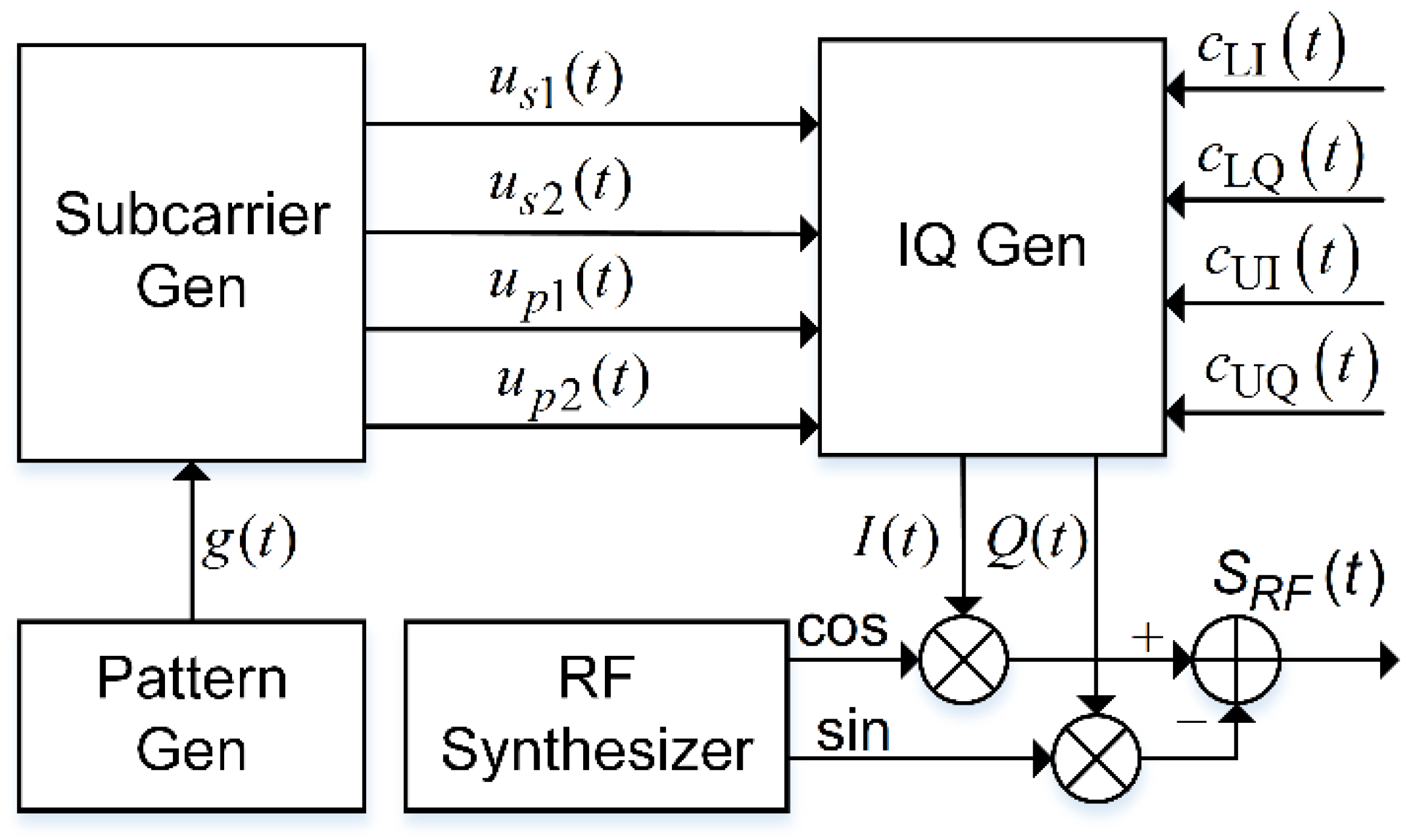
4.1. Direct Generation

The ACE-FHBOC signal can be directly generated according to (11) or its decomposed form, thus, there are two direct methods to generate ACE-FHBOC.

4.1.1. Direct Generation with Composed Subcarriers

As expressed in (11) the waveforms of both the real and imaginary parts for $s_{\mathrm{A}}\left(t\right)$ are square waves, which are functions with $g\left(t\right)$, ${\alpha }_i\left(t\right)$, and ${\phi }_i\left(t\right)$ with $i\in \left\{\mathrm{I},\mathrm{Q}\right\}$. Figure 3 shows the scheme of direct generation with composed subcarriers. According to the signal state and frequency-hopping pattern, the parameters of generating the subcarriers can be obtained. Then, the amplitudes ${\alpha }_i\left(t\right)$ and the subcarriers are multiplied to obtain the in-phase part $\mathrm{I}\left(t\right)$ and quadrature part $\mathrm{Q}\left(t\right)$. Finally, $\mathrm{I}\left(t\right)$ and $\mathrm{Q}\left(t\right)$, which are modulated on the cosine-phase and the sine-phase radio-frequency carriers, are combined to obtain $s_{RF}\left(t\right)$.

4.1.2. Direct Generation with Decomposed Subcarriers

Figure 4 shows the scheme of direct generation with decomposed subcarriers. First, under the control of the frequency-hopping pattern, the subcarrier generator generates the decomposed subcarriers corresponding to each signal component and IM component. Second, the signal components and IM components are multiplied by the corresponding subcarriers to generate the in-phase part $\mathrm{I}\left(t\right)$ and quadrature parts $\mathrm{Q}\left(t\right)$. Finally, $\mathrm{I}\left(t\right)$ and $\mathrm{Q}\left(t\right)$, which are modulated on the cosine-phased and the sine-phased radio-frequency carriers, are combined to obtain $s_{RF}\left(t\right)$.

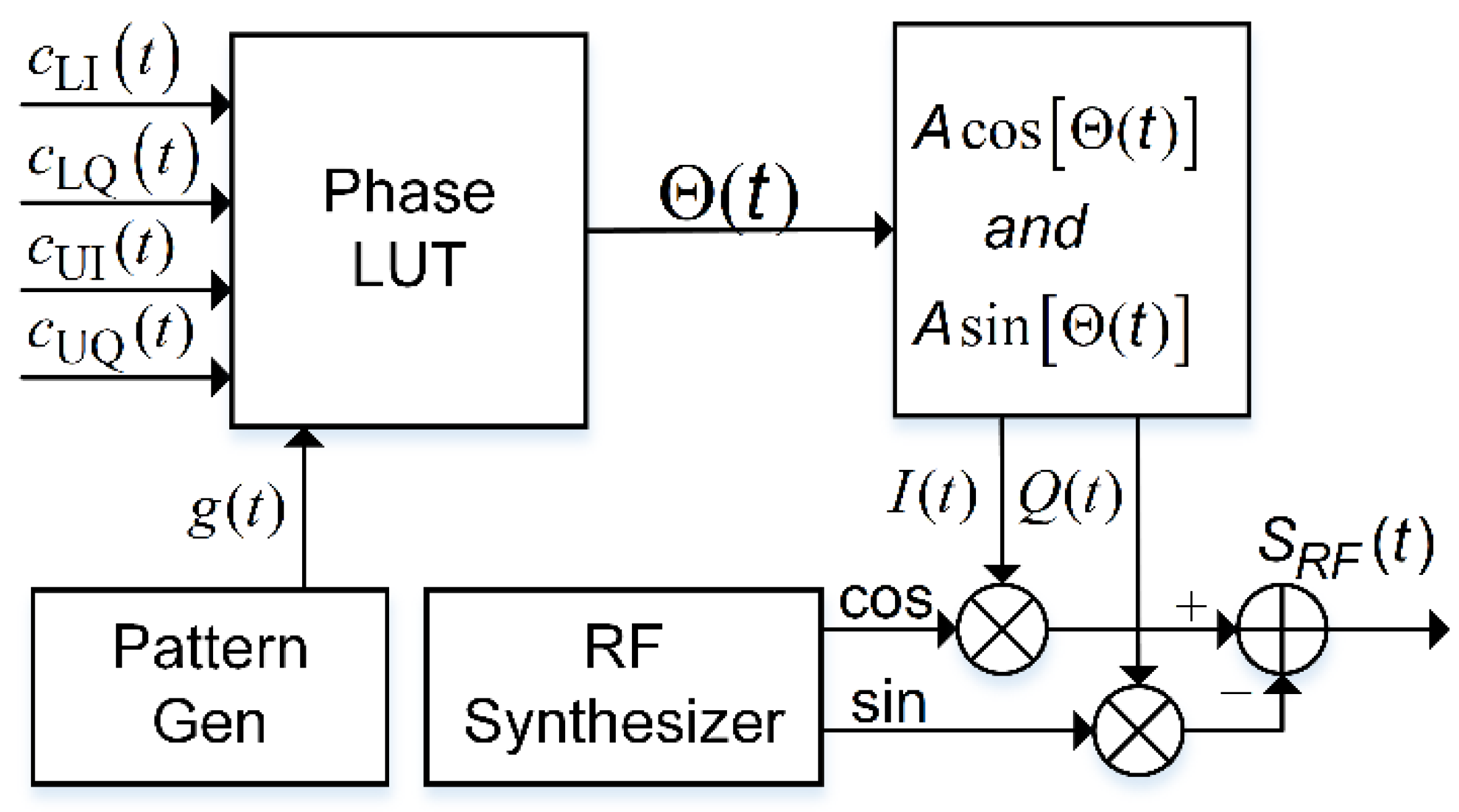
4.2. Phase Rotation Generation

The scheme of phase rotation generation is shown in Figure 5. According to the value of the signal components, frequency-hopping pattern, and time index, $\Theta \left(t\right)$, as the input of the $A\cos \left[\Theta \left(t\right)\right]$ and $A\sin \left[\Theta \left(t\right)\right]$ generator, can be obtained from the phase LUT. Then, the in-phase output $\mathrm{I}\left(t\right)$ and quadrature-phase output $\mathrm{Q}\left(t\right)$ are modulated on the cosine-phased and the sine-phased radio-frequency carriers, respectively. Finally, they are combined to obtain $s_{RF}\left(t\right)$.

The example signal ACE-FHBOC(10:1:1,1), shown in Figure 1, is generated via the direct generation scheme with decomposed subcarriers. The simulated and theoretical normalized ACF results are compared in the top panel of Figure 6, and the simulated and theoretical PSD results are compared in the bottom panel.

4.3. Generation Complexity

Due to the frequency-hopping subcarrier, the generation of ACE-FHBOC generally requires more resources than ACE-BOC. For the sake of clarity, we selected Type-I ACE-FHBOC(${\alpha }_{M-1}$:$d$:${\alpha }_0$, $1$) in comparison with Type-I ACE-BOC($\alpha$, $\beta$).

Table 2. Generation complexity comparison summary.

Resource Consumption	ACE-FHBOC	ACE-BOC
Minimum Subchip Rate	$12{\alpha }_{M-1}{f}_0$	$12\alpha f_0$
Minimum number of Bits of Direct Subcarriers Generator	3	3
LUT of Phase Rotation Generation Method	$M\times 12\times 16$ LUT	$12\times 16$ LUT

lists their generation complexity comparison summary. The minimum number of bits of direct subcarriers generators is three for ACE-FHBOC and ACE-BOC. If the phase rotation generation method is adopted, ACE-BOC, as a special case of ACE-FHBOC, has one subcarrier frequency, which requires $12\times 16$ LUT. However, ACE-FHBOC has $M$ subcarrier frequencies, and the resource consumption of ACE-FHBOC is $M$ times that of ACE-BOC.

5. Performance Analysis

5.1. ACF and PSD

The ACF and PSD are essential in signal simulation, performance evaluation, and acquisition and tracking algorithm design [28,29]. We first derive the expressions of ACF and PSD for each type of ACE-BOC signal. Then, we selected several representative ACE-FHBOC signals in comparison with ACE-BOC. These signals are ACE-FHBOC(24:1:1,1), ACE-FHBOC(24:1:6,1), ACE-BOC(12,1), and ACE-BOC(15,10). ACE-FHBOC(24:1:1,1) has the same PSD main lobe bandwidth (MLB) as ACE-BOC(15,10), and its zero-crossing near the ACF main peak (ZCNM) is approximately equal to that of ACE-BOC(12,1). ACE-FHBOC(24:1:6,1) has the same MLB and ZCNM as ACE-BOC(15,10), and its spectrum compatibility is also similar to ACE-BOC(15,10).

In general, there are two main approaches for processing an ACE-FHBOC: one is to process each signal component independently, and the other is to process the whole ACE-FHBOC signal with a wideband receiver to realize better performance. Under the assumption that an ACE-FHBOC signal has an ideal spreading code and infinite bandwidth, we derive the ACF and PSD of the whole ACE-FHBOC signal in Appendix B.

The top panel of Figure 7 shows the normalized ACFs of the Type-I example signals. ACE-FHBOC(24:1:1,1) has the lowest ACF side peaks among the example signals, which means the lightest ACF ambiguity. The ACF side peaks of ACE-FHBOC(24:1:6,1) are lower than ACE-BOC(15,10). The ACF main peak of ACE-FHBOC(15,10) is the narrowest among the example signals, which means the best potential ranging performance among the example signals. The ACF main peak of ACE-FHBOC(24:1:1,1) is narrower than that of ACE-BOC(12,1).

The bottom panel of Figure 7 shows the normalized PSDs of the Type-I example signals. The power in the PSD main lobes is evenly distributed within the bands for ACE-FHBOC(24:1:1,1), and the maximum value of PSD envelope is the smallest among the example signal. The PSD main lobes of ACE-BOC(12,1), ACE-BOC(15,10), and ACE-FHBOC(24:1:6,1) are offset from the band center.

Table 3. SSCs of the example signals.

${\mathit{K}}_{\mathit{X}\mathit{Y}}$ (dB/Hz)	(12,1)	(15,10)	(24:1:1,1)	(24:1:6,1)
BPSK(1)	−92.2	−83.9	−82.4	−92.0
BPSK(10)	−86.5	−84.2	−78.3	−84.7
MBOC(6,1,1/11)	−92.2	−84.1	−78.5	−86.1
BOC(10,5)	−76.1	−79.4	−78.4	−78.1
Self	−66.7	−76.6	−78.6	−78.0

lists the spectral separation coefficients (SSC) of the example signals with the legacy satellite navigation signals. ACE-FHBOC(24:1:1,1) has a larger cross-SSCs than ACE-BOC(15,10) and ACE-FHBOC(24:1:6,1), but has a smaller self-SSC. Thus, ACE-FHBOC(24:1:1,1) has a worse intersystem compatibility but a better intrasystem compatibility than ACE-BOC(15,10) and ACE-FHBOC(24:1:6,1).

Figure 8 and Figure 9 show the normalized ACFs of the Type-II and Type-III example signals, respectively. Interestingly, the ACFs of these signals are complex. The real parts are even functions and the imaginary parts are odd functions.

Figure 10 shows the normalized PSDs of the Type-II and Type-III example signals, respectively. It can be seen that the upper and lower sidebands are assigned different signal powers.

5.2. Numerical Simulation

To verify the performance of ACE-FHBOC, a computer simulation is carried out based on MATLAB. As is shown in Figure 11, the original navigation signal is first generated. Second, we add noise and interference signals to the original signal. Then, after filtering and sampling, the digital intermediate frequency (IF) signal is generated. Finally, the IF signal is processed by a software-defined receiver (SDR) that is developed based on a generic GNSS SDR [30].

Table 4. Common parameters of the simulated signal.

Parameters	Value
Signal Power Ratio	[1,1,3,3]
Data Rate	50 bit/s
Length of Spreading Code	10230
Length of Frequency-hopping Pattern	10230
Sampling Frequency	286.44 MHz
Intermediate Frequency	71.61 MHz
Filter Bandwidth	50 MHz
Simulated Signal Duration	100 ms
Data Type of Sampled Signal	Eight bit signed char values

lists the main parameters of the simulated signal. According to the acquisition and tracking results of the SDR, we discuss the multiplexing performance, the probabilities of false locking on ACF side peaks, the tracking performance, the anti-narrowband interference performance, and the multipath performance for ACE-FHBOC(24:1:1,1), ACE-FHBOC(24:1:6,1), ACE-BOC(12,1), and ACE-BOC(15,10).

5.2.1. Multiplexing Efficiency

Multiplexing efficiency represents the power proportion of useful signal components in the whole constant-envelope signal, which is not only influenced by the IM power in the ACE-FHBOC but also depends on the receiving strategy. If the whole ACE-FHBOC signal can be reproduced for a local replica and processed with a wideband receiver, the multiplexing efficiency can reach 100%. Another strategy is to receive each signal component independently with a local replica of the corresponding subcarrier in the decomposed form of ACE-FHBOC. For the second strategy, the multiplexing efficiency is defined as

$$\eta =\frac{{\displaystyle \sum _i{R}_i^2\left(0\right)}}{A^2},\hspace{0.17em}\hspace{0.17em}i\in \left\{\mathrm{UI},\mathrm{LI},\mathrm{UQ},\mathrm{LQ}\right\}$$

(27)

where $A$ is the amplitude of the multiplexed signal. $R_i\left(t\right)$ is the autocorrelation for the $i\mathrm{th}$ signal component. Figure 12 shows the multiplexing efficiency versus power ratio ${\beta }^2$. It is evident that Type-I, Type-II, and Type-III ACE-FHBOC and ACE-BOC have the same multiplexing efficiency. A larger power ratio ${\beta }^2$ means higher multiplexing efficiency.

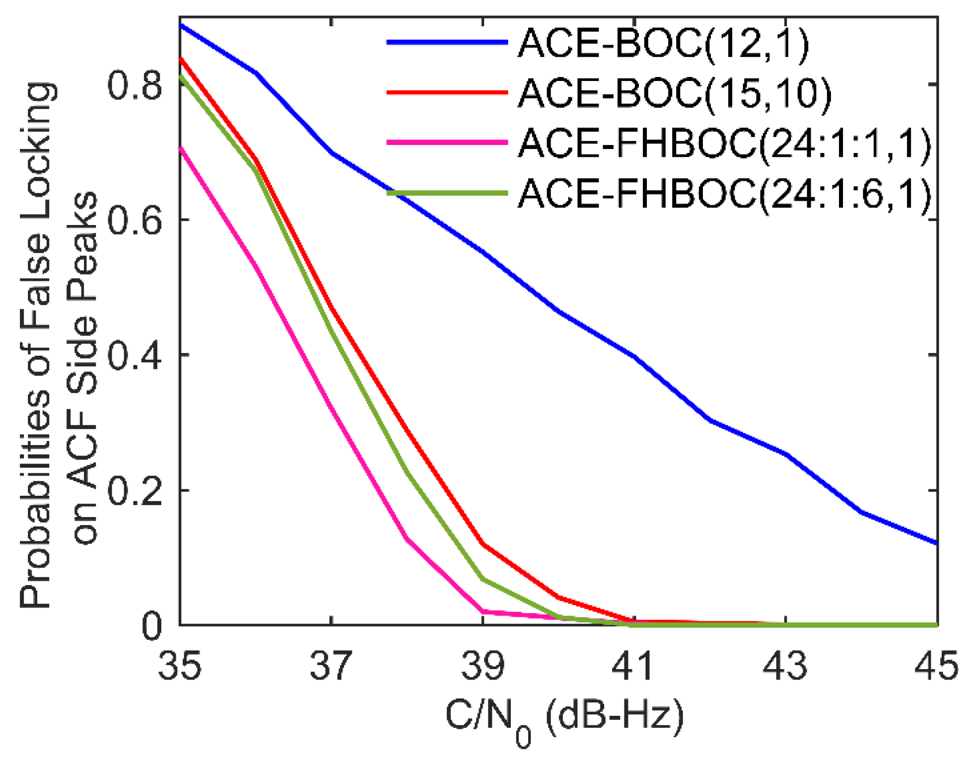
5.2.2. Probability of False Locking on ACF Side Peaks

Low ACF side peak ambiguity is an important advantage of ACE-FHBOC compared to ACE-BOC. To explore the ACF peak ambiguity for the example signals during signal acquisition, we conduct a Monte Carlo simulation. For an early-late spacing of 10.2 ns for ACE-BOC(12,1), 8.15 ns for ACE-BOC(15,10) and ACE-FHBOC(24:1:6,1), 9.8 ns for ACE-FHBOC(24:1:1,1), and a coherent integration time of 1 ms, Figure 13 shows the probabilities of false locking on ACF side peaks versus carrier-to-noise density ratio ($C/N_0$) for the example signals. ACE-FHBOC(24:1:1,1) has the smallest false locking probability among the example signals, whereas ACE-BOC(12,1) has the largest. ACE-FHBOC(24:1:6,1) has a smaller false locking probability than ACE-BOC(15,10).

5.2.3. Tracking Performance

The code tracking for the SDR relies on a discriminator based on noncoherent early-late processing (NELP) [31]. For an early-late spacing of 10.2 ns for ACE-BOC(12,1), 8.15 ns for ACE-BOC(15,10) and ACE-FHBOC(24:1:6,1), 9.8 ns for ACE-FHBOC(24:1:1,1), a coherent integration time of 1 ms, a one-side equivalent rectangular bandwidth of the code tracking loop of 1 Hz, and interference power of zero, Figure 14 shows the simulated code tracking errors versus $C/N_0$ for the example signals. The tracking error for ACE-BOC(15,10) is the smallest among the example signals. The tracking error for ACE-FHBOC(24:1:1,1) is larger than ACE-FHBOC(24:1:6,1) but smaller than ACE-BOC(12,1).

5.2.4. Anti-Narrowband Interference Performance

GNSS signals are vulnerable to interference, resulting in performance degradation [32,33]. A modulation scheme with better anti-interference performance could improve signal tracking performance. We compare the anti-narrowband interference performance for the example signals.

Processing gain is an important index to reflect anti-interference performance for a spread spectrum signal. A larger processing gain means better anti-interference performance. The processing gain for ACE-BOC($\alpha$, $\beta$, $p$) can be expressed as

$$G_{\mathrm{ACE}-\mathrm{BOC}}\approx 10\log (\beta \times \frac{f_0}{f_D})+3$$

(28)

where $f_D$ is the data rate. The processing gain for ACE-FHBOC(${\alpha }_{M-1}$:1:${\alpha }_0$, $\beta$, $p$) is

$$G_{\mathrm{ACE}-\mathrm{FHBOC}}\approx 10\log \left(\beta \times \frac{f_0}{f_D}\right)+10\log \left(\frac{{\alpha }_{M-1}-{\alpha }_0}{\beta }+1\right)+3$$

(29)

The processing gain for ACE-FHBOC(${\alpha }_{M-1}$:1${\alpha }_0$, $\beta$, $p$) is $10\log \left[\left({\alpha }_{M-1}-{\alpha }_0\right)/\beta +1\right]$ dB higher than that for ACE-BOC($\alpha$, $\beta$, $p$). The processing gains for the example signals are listed in

Table 5. Processing gain for the example signals.

Parameters	(24:1:1,1)	(24:1:6,1)	(15,10)	(12,1)
$G$ (dB)	59.9	58.9	56.1	46.1

. ACE-FHBOC(24:1:1,1) has the largest processing gain, and ACE-BOC(12,1) has the smallest. The processing gain for ACE-FHBOC(24:1:6,1) is 2.8 dB larger than that for ACE-BOC(15,10).

To verify the anti-narrowband interference performance for the example signals, we conduct a simulation. The interference signal is assumed to be a periodic chirp signal, defined as follows:

$$I(t)=A\cos \left(2\pi f_{I}t\pm \pi \frac{B_I}{T_I}{t}^2+{\phi }_0\right),\hspace{0.17em}\hspace{0.17em}-\frac{T_I}{2}<t<\frac{T_I}{2}$$

(30)

where $A$ is the amplitude, and $f_I$ is the center frequency of the chirp, $T_I$ is the chirp duration, $B_I$ is the sweeping bandwidth. It is assumed that the $B_I$ of the chirp is 1 MHz and $T_I$ is 0.1 ms in the simulation.

For an early-late spacing of 10.2 ns for ACE-BOC(12,1), 8.15 ns for ACE-BOC(15,10) and ACE-FHBOC(24:1:6,1), 9.8 ns for ACE-FHBOC(24:1:1,1), a coherent integration time of 1 ms, a one-side equivalent rectangular bandwidth of the code tracking loop of 1 Hz, $C/N_0$ of 43 dB, and the chirp interference whose center frequency located at the center of the main lobes of the signal, the simulated tracking errors versus the ratio of interference power to signal power for the example signals are shown in Figure 15. The differences in the processing gains for the example signals are evident. ACEBOC(24:1:1,1) is the most resistant to interference among the example signals. ACE-FHBOC(24:1:6,1) is more resistant to interference than ACE-BOC(15,10).

5.2.5. Multipath Performance

Multipath interference is one of the main sources of error in satellite navigation [34]. For a multipath situation with one direct path and one reflected path with a multipath-to-direct ratio of −6 dB, an early-late spacing of 10.2 ns for ACE-BOC(12,1), 8.15 ns for ACE-BOC(15,10) and ACE-FHBOC(24:1:6,1), 9.8 ns for ACE-FHBOC(24:1:1,1), Figure 16 shows the simulated NELP multipath error envelopes versus the multipath delay for the example signal. When the multipath delay is less than 30 m, the most common multipath delay in urban environments [35], the error envelopes for ACE-FHBOC(24:1:1,1) is the smallest among the example signals, and the error envelopes for ACE-FHBOC(24:1:6,1) are smaller than those for ACE-BOC(15,10) and ACE-BOC(12,1).

6. Conclusions

In order to combine several FH-BOC signal components into a constant-envelope signal, we propose ACE-FHBOC modulation that is not only a generalized ACE-BOC but also a multicarrier constant-envelope multiplexing modulation. The ACE-FHBOC provides higher design flexibility in the number of subcarrier frequencies than ACE-BOC while maintaining the same flexibility of signal design as ACE-BOC in the number of signal components and power ratio among components. The subcarrier frequencies of ACE-FHBOC can be flexibly specified by changing the frequency-hopping pattern, and the number and power of its signal components can be allocated by adjusting the power ratio vector. The number of the signal components of ACE-FHBOC ranges from 1 to 4.

There are two expression forms of ACE-FHBOC, namely the time domain form and the phase domain form, which can be converted to each other. The time domain form is intuitive and easy to understand, while the phase domain form can be implemented flexibly and conveniently in hardware. According to these two expression forms, we give two signal generation schemes, which are direct generation and phase rotation generation. As a generalized modulation of ACE-BOC, the generation schemes of ACE-FHBOC can be implemented based on those of ACE-BOC with minor modifications. Due to the frequency-hopping subcarrier, the generation of the ACE-FHBOC generally requires more resources than ACE-BOC.

In addition, the performance analysis of ACE-FHBOC by comparing different example signals of ACE-FHBOC and ACE-BOC is conducted. The frequency-hopping pattern and power ratio vector determine the shapes of ACF and PSD of an ACE-FHBOC signal, which affect the measurement performance and spectrum compatibility of the signal. Therefore, we can shape the ACF and PSD according to the signal performance index by adjusting the frequency-hopping pattern and power ratio vector. The numerical simulation results show that ACE-FHBOC and ACE-BOC have the same multiplexing efficiency. The probabilities of false locking on ACF side peaks of ACE-FHBOC is lower than that of ACE-BOC under the same condition because ACE-FHBOC has a lower ACF side peak ambiguity. Furthermore, the tracking error of ACE-BOC is smaller than that of ACE-FHBOC under the same condition. But the anti-narrowband interference and multipath performance of ACE-FHBOC is better than that of ACE-BOC under the same condition.

ACE-FHBOC is essentially a hybrid DS/FH spread spectrum modulation, which inherits the advantages of the direct-sequence spread spectrum and the frequency-hopping spread spectrum. Unlike the traditional DS/FH signal, the ACE-FHBOC signal is multilevel and can be realized digitally. Furthermore, the performance for carrier phase measurements and Doppler measurements is not affected because the frequency hopping for ACE-FHBOC is implemented in subcarriers. Since ACE-FHBOC has a two-dimensional multiple access space, it enables more multiple accesses than ACE-BOC. ACE-FHBOC improves the flexibility of GNSS signal design and has advantages in low ACF ambiguity and anti-interference, which can be used in new generation GNSS signal design, especially military signal design. With high design flexibility, it can also be used in signal design for GNSS-like systems.

References

1. Zhu, N.; Marais, J.; Bétaille, D.; Berbineau, M. GNSS position integrity in urban environments: A review of literature. IEEE Trans. Intell. Transport. Syst. 2018, 19, 2762–2778. [Google Scholar] [CrossRef] [Green Version]
2. Causa, F.; Fasano, G. Improving navigation in GNSS-challenging environments: Multi-UAS cooperation and generalized dilution of precision. IEEE Trans. Aerosp. Electron. Syst. 2020, 57, 1462–1479. [Google Scholar] [CrossRef]
3. Chiang, K.-W.; Le, D.T.; Duong, T.T.; Sun, R. The performance analysis of INS/GNSS/V-SLAM integration scheme using smartphone sensors for land vehicle navigation applications in GNSS-challenging environments. Remote Sens. 2020, 12, 1732. [Google Scholar] [CrossRef]
4. Ye, L.; Yang, Y.; Jing, X.; Ma, J.; Deng, L.; Li, H. Single-Satellite Integrated Navigation Algorithm Based on Broadband LEOConstellation Communication Links. Remote Sens. 2021, 13, 703. [Google Scholar] [CrossRef]
5. Ma, J.G.; Yang, Y.K.; Li, H.N.; Li, J.S. FH-BOC: Generalized low-ambiguity anti-interference spread spectrum modulation based on frequency-hopping binary offset carrier. GPS Solut. 2020, 24, 70. [Google Scholar] [CrossRef]
6. Yao, Z.; Lu, M.Q. Signal multiplexing techniques for GNSS: The principle, progress, and challenges within a uniform framework. IEEE Signal Process Mag. 2017, 34, 16–26. [Google Scholar] [CrossRef]
7. Xue, L.; Li, X.; Wu, W.; Dong, J. Multifunctional Signal Design for Measurement, Navigation and Communication Based on BOC and BPSK Modulation. Remote Sens. 2022, 14, 1653. [Google Scholar] [CrossRef]
8. Yao, Z.; Lu, M.Q. Next-Generation GNSS Signal Design: Theories, Principles, and Technologies; Springer Nature: Berlin/Heidelberg, Germany, 2021. [Google Scholar]
9. Butman, S.; Timor, U. Interplex—An efficient multichannel PSK/PM telemetry system. IEEE Trans. Commun. 1972, 20, 415–419. [Google Scholar] [CrossRef]
10. Spilker, J.J.; Orr, R.S. Code multiplexing via majority logic for GPS modernization. In Proceedings of the ION GPS 1998, Institute of Navigation, Nashville, TN, USA, 15–18 September 1998; pp. 265–273. [Google Scholar]
11. Dafesh, P.; Nguyen, T.; Lazar, S. Coherent adaptive subcarrier modulation (CASM) for GPS modernization. In Proceedings of the ION NTM 1999, San Diego, CA, USA, 25–27 January 1999; pp. 649–660. [Google Scholar]
12. Dafesh, P.; Cahn, C. Phase-optimized constant-envelope transmission (POCET) modulation method for GNSS signals. In Proceeding of the ION GNSS 2009, Savannah, GA, USA, 22–25 September 2009; pp. 2860–2866. [Google Scholar]
13. Yan, T.; Tang, Z.P.; Wei, J.L.; Qu, B.; Zhou, Z.H. A Quasi-constant Envelope Multiplexing Technique for GNSS Signals. J. Navig. 2015, 68, 791–808. [Google Scholar] [CrossRef] [Green Version]
14. Lestarquit, L.; Artaud, G.; Issler, J.L. AltBOC for dummies or everything you always wanted to know about AltBOC. In Proceedings of the ION GNSS 2008, Savannah, GA, USA, 16–19 September 2008; pp. 961–970. [Google Scholar]
15. Tang, Z.P.; Zhou, H.; Wei, J.L.; Yan, T.; Liu, Y.Q.; Ran, Y.J.; Zhou, Y.L. TD-AltBOC: A new COMPASS B2 modulation. In Proceedings of the China Satellite Navigation Conference 2010, Shanghai, China, 18–22 October 2010. [Google Scholar]
16. Zhu, L.; Yao, Z.; Lu, M.Q.; Feng, Z. Non-symmetrical AltBOC multiplexing for Compass B1 signal design. J. Tsinghua Univ. 2012, 52, 869–873. [Google Scholar]
17. Zhang, K. Generalised constant-envelope DualQPSK and AltBOC modulations for modern GNSS signals. Electron. Lett. 2013, 49, 1335–1337. [Google Scholar] [CrossRef]
18. Zhang, K.; Zhou, H.; Wang, F. Unbalanced AltBOC: A Compass B1 candidate with generalized MPOCET technique. GPS Solut. 2013, 17, 153–164. [Google Scholar] [CrossRef]
19. Yao, Z.; Lu, M.Q. Design, Implementation, and Performance Analysis of ACE-BOC Modulation. In Proceedings of the ION GNSS+ 2013, Nashville, TN, USA, 16–20 September 2013; pp. 361–368. [Google Scholar]
20. Huang, X.; Zhu, X.; Tang, X.; Gong, H.; Ou, G. GCE-BOC modulation: A generalized multiplexing technology for modern GNSS dual-frequency signals. In Proceedings of the China satellite navigation conference (CSNC) 2015, Xi’an, China, 13–15 May 2015; pp. 47–55. [Google Scholar]
21. Yan, T.; Wei, J.L.; Tang, Z.P.; Zhou, Z. General AltBOC Modulation with Adjustable Power Allocation Ratio for GNSS. J. Navig. 2016, 69, 531–560. [Google Scholar] [CrossRef] [Green Version]
22. Yao, Z.; Zhang, J.; Lu, M.Q. ACE-BOC dual-frequency constant envelope multiplexing for satellite navigation. IEEE Trans. Aerosp. Electron. Syst. 2016, 52, 466–485. [Google Scholar] [CrossRef]
23. Guo, F.; Yao, Z.; Lu, M.Q. BS-ACEBOC: A generalized low-complexity dual-frequency constant-envelope multiplexing modulation for GNSS. GPS Solut. 2017, 21, 561–575. [Google Scholar] [CrossRef]
24. Dafesh, P.A.; Cahn, C.R. Application of POCET Method to Combine GNSS Signals at Different Carrier Frequencies. In Proceedings of the ION ITM 2011, San Diego, CA, USA, 24–26 January 2011; pp. 1201–1206. [Google Scholar]
25. Yao, Z.; Guo, F.; Ma, J.; Lu, M.Q. Orthogonality-based generalized multicarrier constant envelope multiplexing for DSSS signals. IEEE Trans. Aerosp. Electron. Syst. 2017, 53, 1685–1698. [Google Scholar] [CrossRef]
26. Ma, J.; Yao, Z.; Lu, M.Q. Multicarrier Constant-Envelope Multiplexing Technique by Subcarrier Vectorization for New Generation GNSSs. IEEE Commun. Lett. 2019, 23, 991–994. [Google Scholar] [CrossRef]
27. Zhang, X.; Zhang, X.; Yao, Z.; Lu, M.Q. Implementations of constant envelope multiplexing based on extended Interplex and inter-modulation construction method. In Proceedings of the ION GNSS 2012, Nashville, TN, USA, 17–21 September 2012; pp. 1201–1206. [Google Scholar]
28. Xie, G. Principle of GNSS: GPA, GLONASS, and Galileo; Publishing House of Electronics Industry: Beijing, China, 2013; p. 54. [Google Scholar]
29. Sousa, F.M.; Nunes, F.D. New expressions for the autocorrelation function of BOC GNSS signals. NAVIGATION J. Inst. Navig. 2013, 60, 1–9. [Google Scholar] [CrossRef]
30. Borre, K.; Akos, D.M.; Bertelsen, N.; Rinder, P.; Jensen, S.H. A Software-Defined GPS and Galileo Receiver: A Single-Frequency Approach; Springer Science & Business Media: Berlin/Heidelberg, Germany, 2007. [Google Scholar]
31. Betz, J.W.; Kolodziejski, K.R. Generalized theory of code tracking with an early-late discriminator part II: Noncoherent processing and numerical results. IEEE Trans. Aerosp. Electron. Syst. 2009, 45, 1557–1564. [Google Scholar] [CrossRef]
32. Zhang, J.; Cui, X.; Xu, H.; Lu, M. A Two-Stage Interference Suppression Scheme Based on Antenna Array for GNSS Jamming and Spoofing. Sensors 2019, 19, 3870. [Google Scholar] [CrossRef] [Green Version]
33. Qin, W.; Gamba, M.T.; Falletti, E.; Dovis, F. An assessment of impact of adaptive notch filters for interference removal on the signal processing stages of a GNSS receiver. IEEE Trans. Aerosp. Electron. Syst. 2020, 56, 4067–4082. [Google Scholar] [CrossRef]
34. Huang, L.; Lu, Z.; Xiao, Z.; Ren, C.; Song, J.; Li, B. Suppression of Jammer Multipath in GNSS Antenna Array Receiver. Remote Sens. 2022, 14, 350. [Google Scholar] [CrossRef]
35. Hein, G.W.; Avila-Rodriguez, J.-A.; Wallner, S.; Pratt, A.R.; Owen, J.; Issler, J.; Betz, J.W.; Hegarty, C.J.; Lenahan, S.; Rushanan, J.J.; et al. MBOC: The new optimized spreading modulation recommended for GALILEO L1 O.S. and GPS L1C. In Proceedings of the IEEE/ION PLANS 2006, San Diego, CA, USA, 25–27 April 2006; pp. 883–892. [Google Scholar]
Figure 1. Waveforms of the real part and the imaginary part for the example signal.
Remotesensing 14 03871 g001
Figure 2. Modulation constellation for the example signal.
Remotesensing 14 03871 g002
Figure 3. Direct generation with composed subcarriers.
Remotesensing 14 03871 g003
Figure 4. Direct generation with decomposed subcarriers.
Remotesensing 14 03871 g004
Figure 5. Phase rotation generation.
Remotesensing 14 03871 g005
Figure 6. Simulated and theoretical results for normalized ACF and PSD of ACE-FHBOC(10:1:1,1).
Remotesensing 14 03871 g006
Figure 7. Normalized ACFs and PSDs of the Type-I example signals.
Remotesensing 14 03871 g007
Figure 8. Normalized ACFs of the Type-II example signals.
Remotesensing 14 03871 g008
Figure 9. Normalized ACFs of the Type-III example signals.
Remotesensing 14 03871 g009
Figure 10. PSDs of the Type-II and Type-III example signals.
Remotesensing 14 03871 g010
Figure 11. Simulation scheme.
Remotesensing 14 03871 g011
Figure 12. Multiplexing efficiency of Type-I, -II, and –III ACE-FHBOC and ACE-BOC.
Remotesensing 14 03871 g012
Figure 13. Probabilities of false locking on ACF side peaks for the example signals.
Remotesensing 14 03871 g013
Figure 14. NELP code tracking errors for the example signals.
Remotesensing 14 03871 g014
Figure 15. Tracking errors for the example signals.
Remotesensing 14 03871 g015
Figure 16. NELP multipath errors for the example signals.
Remotesensing 14 03871 g016