
An Illumination-Invariant Shadow-Based Scene Matching Navigation Approach in Low-Altitude Flight


 ,
,  and
and
Abstract
:
1. Introduction
2. Related Work
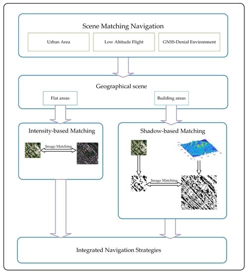
3. Problem Description
4. Methodology
4.1. Consistency of Shadow in Orthophoto
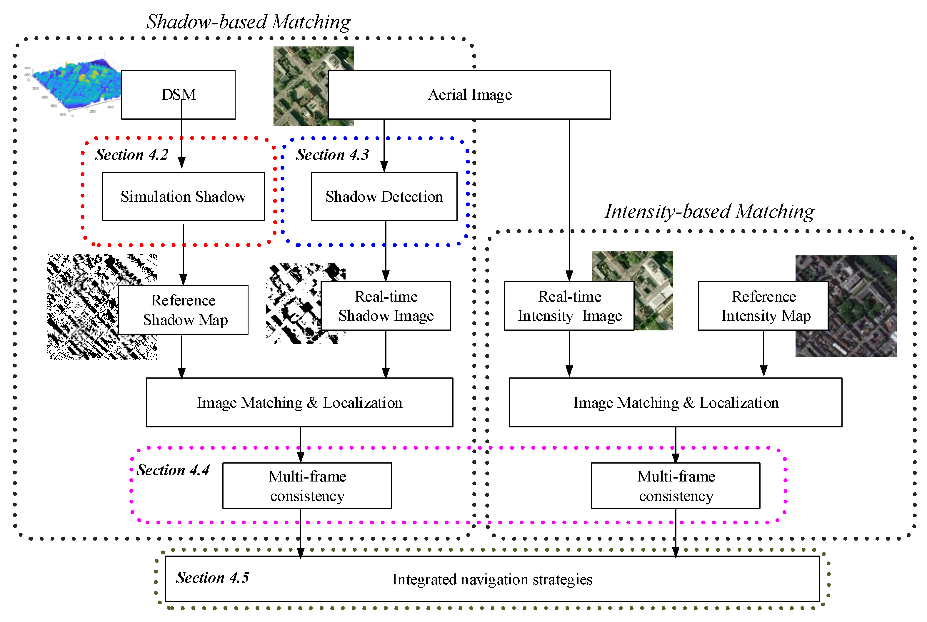
4.2. Generation of the Reference Shadow Map
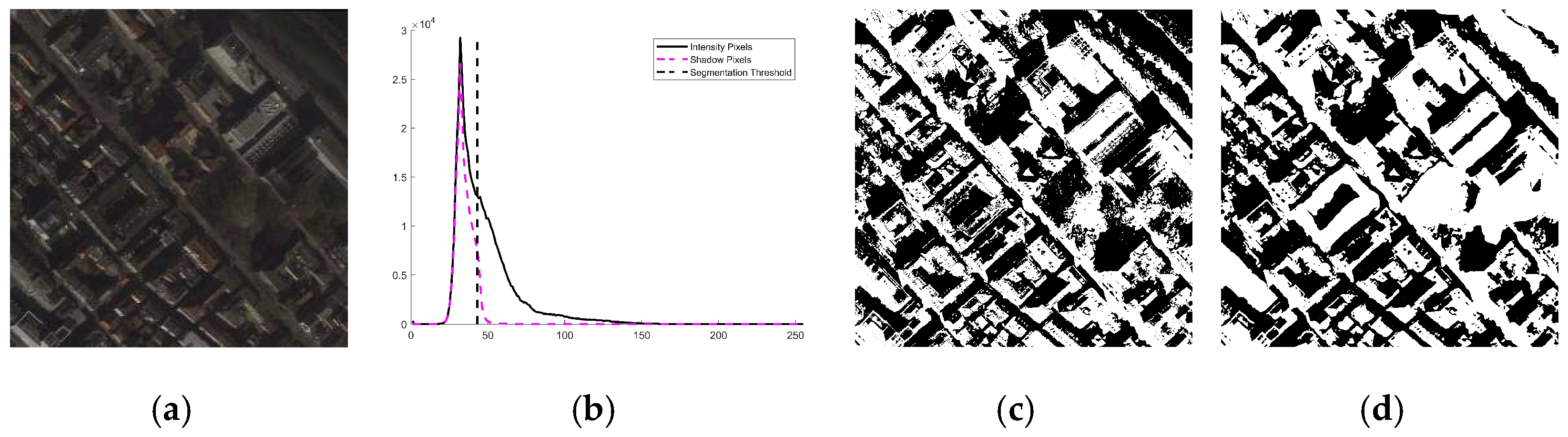
4.3. Shadow Detection from Aerial Photos
- Find the first valley in respective red, green, and blue channels.
- (a)
- Assume that is the valley width parameter. The initial value is set to 9.
- (b)
- Find the minimum on the histogram of the channel image with the parameter satisfying the following condition:If exists, the histogram distribution is not unimodal and the value of is found. Otherwise, go to sub-step c.
- (c)
- Make , if (), repeat sub-step b, or else set to 256, to indicate that the search for has failed with any and that the histogram of the channel is unimodal.After the “first valley” is detected for each channel, the thresholds , , and of red, green, and blue channels can be obtained.
- If at least one channel is not unimodal, the final shadow image can be obtained by the intersection of the three-channel shadow images , , and , i.e.,
- If all three channels are unimodal, the range-constrained Otsu method [54] is applied in the combined channel ():
- (a)
- Evaluate the threshold by the Otsu method [45] in the whole image .
- (b)
- Evaluate the threshold by the Otsu method in the pixels with the range in .
- (c)
- Then, the final shadow image can be produced by .
4.4. Scene Matching with Constraints Based on Multi-Frame Consistency
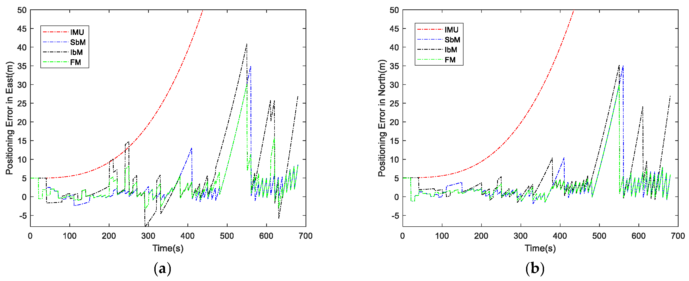
4.5. Integrated Navigation Strategies
- If one of the results of SbM and IbM is available, the available one is used.
- If both the results of SbM and IbM are available, the final matching result is the arithmetic mean of both.
- If neither the results of SbM nor IbM are available, the position update is based on IMU only.
5. Experimental Results
5.1. Data Acquisition and Evaluation Metrics
- Satellite images from Google Earth that have a spatial resolution of 0.5 m. Photographs from Google Earth are used to test shadow detection algorithms and in navigation experiments as geo-referenced images.
- Ground truth of shadow images for assessment of the shadow detection algorithm. All images used in the evaluation of the shadow detection algorithm were manually calibrated to generate the corresponding ground truth shadow images.
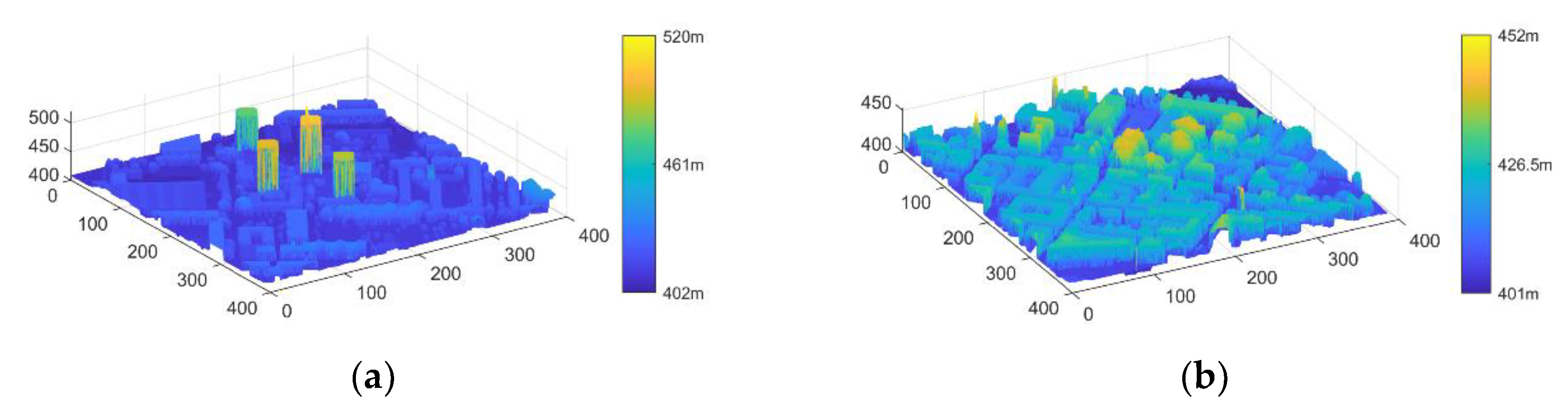
- Rasterized DSM data at 0.5 m spatial resolution from the GIS information project of the cantonal government of Zurich (http://maps.zh.ch/, accessed on 18 March 2021).
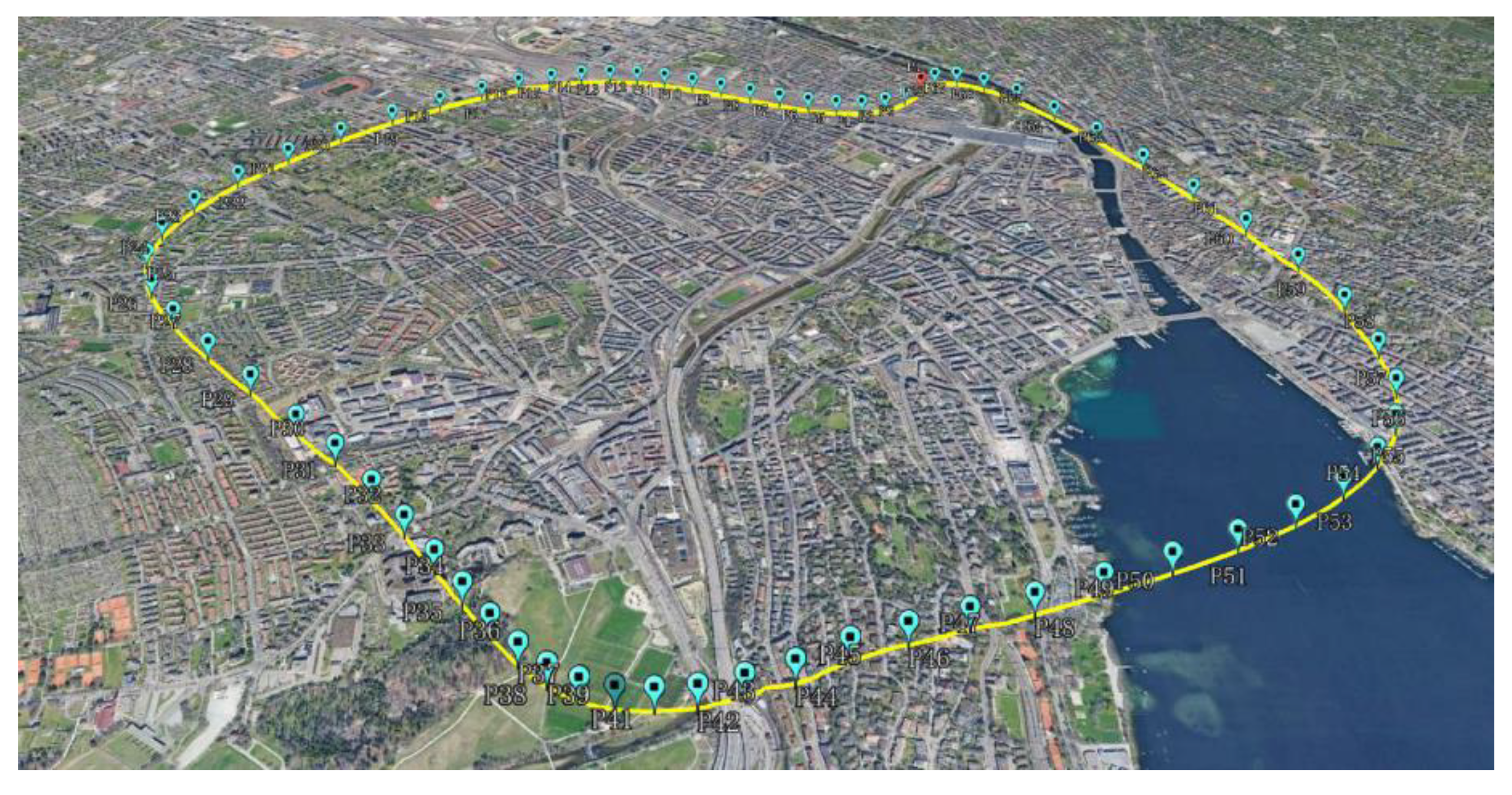
- Downward-looking aerial image with a resolution of 0.25 m taken in the summer of 2018 over Zurich. In the navigation experiment, this aerial photograph was used as a real-time image.
5.2. Shadow Detection and Evaluation
5.3. Simulation and Experiment
6. Discussion
7. Conclusions
Author Contributions
Funding
Data Availability Statement
Conflicts of Interest
References
- Grewal, M.S.; Weill, L.R.; Andrews, A.P. Global Positioning Systems, Inertial Navigation, and Integration; John Wiley & Sons: New York, NY, USA, 2007; ISBN 0470099712. [Google Scholar]
- Tang, Y.; Jiang, J.; Liu, J.; Yan, P.; Tao, Y.; Liu, J. A GRU and AKF-Based Hybrid Algorithm for Improving INS/GNSS Navigation Accuracy during GNSS Outage. Remote Sens. 2022, 14, 752. [Google Scholar] [CrossRef]
- Piasco, N.; Sidibé, D.; Demonceaux, C.; Gouet-Brunet, V. A survey on Visual-Based Localization: On the benefit of heterogeneous data. Pattern Recognit. 2018, 74, 90–109. [Google Scholar] [CrossRef]
- Kim, Y.; Park, J.; Bang, H. Terrain-Referenced Navigation using an Interferometric Radar Altimeter. Navig. J. Inst. Navig. 2018, 65, 157–167. [Google Scholar] [CrossRef]
- Jin, Z.; Wang, X.; Moran, B.; Pan, Q.; Zhao, C. Multi-Region Scene Matching Based Localisation for Autonomous Vision Navigation of UAVs. J. Navig. 2016, 69, 1215–1233. [Google Scholar] [CrossRef]
- Choi, S.H.; Park, C.G. Robust aerial scene-matching algorithm based on relative velocity model. Robot. Auton. Syst. 2020, 124, 103372. [Google Scholar] [CrossRef]
- Qu, X.; Soheilian, B.; Paparoditis, N. Landmark based localization in urban environment. ISPRS J. Photogramm. Remote Sens. 2018, 140, 90–103. [Google Scholar] [CrossRef]
- Wan, X.; Liu, J.; Yan, H.; Morgan, G.L.K. Illumination-invariant image matching for autonomous UAV localisation based on optical sensing. ISPRS J. Photogramm. Remote Sens. 2016, 119, 198–213. [Google Scholar] [CrossRef]
- Nistér, D.; Naroditsky, O.; Bergen, J. Visual Odometry. In Proceedings of the 2004 IEEE Computer Society Conference on Computer Vision and Pattern Recognition, Washington, DC, USA, 27 June–2 July 2004; IEEE: Piscataway, NJ, USA, 2004; Volume 1, p. I. [Google Scholar]
- Mur-Artal, R.; Montiel, J.M.M.; Tardos, J.D. ORB-SLAM: A Versatile and Accurate Monocular SLAM System. IEEE Trans. Robot. 2015, 31, 1147–1163. [Google Scholar] [CrossRef]
- Forster, C.; Pizzoli, M.; Scaramuzza, D. SVO: Fast semi-direct monocular visual odometry. In Proceedings of the 2014 IEEE International Conference on Robotics and Automation (ICRA), Hong Kong, China, 31 May–7 June 2014; pp. 15–22. [Google Scholar] [CrossRef]
- Brown, L.G. A survey of image registration techniques. ACM Comput. Surv. 1992, 24, 325–376. [Google Scholar] [CrossRef]
- Shukla, P.K.; Goel, S.; Singh, P.; Lohani, B. Automatic geolocation of targets tracked by aerial imaging platforms using satellite imagery. Int. Arch. Photogramm. Remote Sens. Spat. Inf. Sci. ISPRS Arch. 2014, XL-1, 381–388. [Google Scholar] [CrossRef]
- Jacobsen, K. Very High Resolution Satellite Images—Competition to Aerial Images. 2009. Available online: https://www.ipi.uni-hannover.de/fileadmin/ipi/publications/VHR_Satellites_Jacobsen.pdf (accessed on 8 March 2022).
- Zhuo, X.; Koch, T.; Kurz, F.; Fraundorfer, F.; Reinartz, P. Automatic UAV Image Geo-Registration by Matching UAV Images to Georeferenced Image Data. Remote Sens. 2017, 9, 376. [Google Scholar] [CrossRef]
- Yoo, J.-C.; Han, T.H. Fast Normalized Cross-Correlation. Circuits Syst. Signal Process. 2009, 28, 819–843. [Google Scholar] [CrossRef]
- Mo, N.; Zhu, R.; Yan, L.; Zhao, Z. Deshadowing of Urban Airborne Imagery Based on Object-Oriented Automatic Shadow Detection and Regional Matching Compensation. IEEE J. Sel. Top. Appl. Earth Obs. Remote Sens. 2018, 11, 585–605. [Google Scholar] [CrossRef]
- Wang, H.; Cheng, Y.; Liu, N.; Kang, Z. A Method of Scene Matching Navigation in Urban Area Based on Shadow Matching. In Proceedings of the 2018 IEEE CSAA Guidance, Navigation and Control Conference (CGNCC), Xiamen, China, 10–12 August 2018; pp. 1–6. [Google Scholar] [CrossRef]
- Wan, X.; Liu, J.G.; Yan, H. The Illumination Robustness of Phase Correlation for Image Alignment. IEEE Trans. Geosci. Remote Sens. 2015, 53, 5746–5759. [Google Scholar] [CrossRef]
- Movia, A.; Beinat, A.; Crosilla, F. Shadow detection and removal in RGB VHR images for land use unsupervised classification. ISPRS J. Photogramm. Remote Sens. 2016, 119, 485–495. [Google Scholar] [CrossRef]
- Song, L.; Cheng, Y.M.; Liu, N.; Song, C.H.; Xu, M. A Scene Matching Method Based on Weighted Hausdorff Distance Combined with Structure Information. In Proceedings of the 32nd Chinese Control Conference, Xi’an, China, 26–28 July 2013; pp. 5241–5244. [Google Scholar]
- Sim, D.-G.; Park, R.-H. Two-dimensional object alignment based on the robust oriented Hausdorff similarity measure. IEEE Trans. Image Process. 2001, 10, 475–483. [Google Scholar] [CrossRef]
- Cesetti, A.; Frontoni, E.; Mancini, A.; Zingaretti, P.; Longhi, S. A Vision-Based Guidance System for UAV Navigation and Safe Landing using Natural Landmarks. J. Intell. Robot. Syst. 2010, 57, 233–257. [Google Scholar] [CrossRef]
- Bay, H.; Ess, A.; Tuytelaars, T.; Van Gool, L. Speeded-up robust features (SURF). Comput. Vis. Image Underst. 2008, 110, 346–359. [Google Scholar] [CrossRef]
- Rublee, E.; Rabaud, V.; Konolige, K.; Bradski, G. ORB: An efficient alternative to SIFT or SURF. In Proceedings of the IEEE International Conference on Computer Vision, Barcelona, Spain, 6–13 November 2011; pp. 2564–2571. [Google Scholar] [CrossRef]
- Ma, J.; Jiang, X.; Fan, A.; Jiang, J.; Yan, J. Image matching from handcrafted to deep features: A survey. Int. J. Comput. Vis. 2021, 129, 23–79. [Google Scholar] [CrossRef]
- Lowry, S.; Sunderhauf, N.; Newman, P.; Leonard, J.J.; Cox, D.; Corke, P.; Milford, M.J. Visual Place Recognition: A Survey. IEEE Trans. Robot. 2016, 32, 1–19. [Google Scholar] [CrossRef]
- Krajník, T.; Cristóforis, P.; Kusumam, K.; Neubert, P.; Duckett, T. Image features for visual teach-and-repeat navigation in changing environments. Robot. Auton. Syst. 2017, 88, 127–141. [Google Scholar] [CrossRef]
- Azzalini, D.; Bonali, L.; Amigoni, F. A Minimally Supervised Approach Based on Variational Autoencoders for Anomaly Detection in Autonomous Robots. IEEE Robot. Autom. Lett. 2021, 6, 2985–2992. [Google Scholar] [CrossRef]
- Michaelsen, E.; Meidow, J. Stochastic reasoning for structural pattern recognition: An example from image-based UAV navigation. Pattern Recognit. 2014, 47, 2732–2744. [Google Scholar] [CrossRef]
- Yang, X.; Wang, J.; Qin, X.; Wang, J.; Ye, X.; Qin, Q. Fast Urban Aerial Image Matching Based on Rectangular Building Extraction. IEEE Geosci. Remote Sens. Mag. 2015, 3, 21–27. [Google Scholar] [CrossRef]
- Dawadee, A.; Chahl, J.; Nandagopal, D.; Nedic, Z. Illumination, Scale and Rotation Invariant Algorithm for Vision-Based Uav Navigation. Int. J. Pattern Recognit. Artif. Intell. 2013, 27, 1359003. [Google Scholar] [CrossRef]
- McCabe, J.S.; DeMars, K.J. Vision-based, terrain-aided navigation with decentralized fusion and finite set statistics. Navig. J. Inst. Navig. 2019, 66, 537–557. [Google Scholar] [CrossRef]
- Talluri, R.; Aggarwal, J. Position estimation for an autonomous mobile robot in an outdoor environment. IEEE Trans. Robot. Autom. 1992, 8, 573–584. [Google Scholar] [CrossRef]
- Woo, J.; Son, K.; Li, T.; Kim, G.; Kweon, I.S. Vision-Based UAV Navigation in Mountain Area. In Proceedings of the IAPR Conference on Machine Vision Applications, Tokyo, Japan, 16–18 May 2007; pp. 236–239. [Google Scholar]
- Baboud, L.; Cadik, M.; Eisemann, E.; Seidel, H.-P. Automatic photo-to-terrain alignment for the annotation of mountain pictures. In Proceedings of the IEEE Computer Society Conference on Computer Vision and Pattern Recognition, Colorado Springs, CO, USA, 20–25 June 2011; pp. 41–48. [Google Scholar] [CrossRef]
- Wang, T.; Celik, K.; Somani, A.K. Characterization of mountain drainage patterns for GPS-denied UAS navigation augmentation. Mach. Vis. Appl. 2016, 27, 87–101. [Google Scholar] [CrossRef]
- Taneja, A.; Ballan, L.; Pollefeys, M. Registration of Spherical Panoramic Images with Cadastral 3D Models. In Proceedings of the 2012 Second International Conference on 3D Imaging, Modeling, Processing, Visualization & Transmission, Zurich, Switzerland, 13–15 October 2012; pp. 479–486. [Google Scholar] [CrossRef]
- Ramalingam, S.; Bouaziz, S.; Sturm, P.; Brand, M. SKYLINE2GPS: Localization in urban canyons using omni-skylines. In Proceedings of the 2010 IEEE/RSJ International Conference on Intelligent Robots and Systems, Taipei, Taiwan, 18–22 October 2010; pp. 3816–3823. [Google Scholar] [CrossRef]
- Muja, M.; Lowe, D.G. Fast Approximate Nearest Neighbors with Automatic Algorithm Configuration. In Proceedings of the Fourth International Conference on Computer Vision Theory and Applications, Lisboa, Portugal, 5–8 February 2009; pp. 331–340. [Google Scholar] [CrossRef]
- Ahmar, F.; Jansa, J.; Ries, C. The Generation of True Orthophotos Using a 3D Building Model in Conjunction With a Conventional Dtm. Int. Arch. Photogramm. Remote Sens. 1998, 32, 16–22. [Google Scholar]
- Zhang, T.; Stackhouse, P.W.; Macpherson, B.; Mikovitz, J.C. A Solar Azimuth Formula That Renders Circumstantial Treatment Unnecessary without Compromising Mathematical Rigor: Mathematical Setup, Application and Extension of a Formula Based on the Subsolar Point and Atan2 Function. Renew. Energy 2021, 172, 1333–1340. [Google Scholar] [CrossRef]
- Woo, A. Efficient shadow computations in ray tracing. IEEE Comput. Graph. Appl. 1993, 13, 78–83. [Google Scholar] [CrossRef]
- McCool, M.D. Shadow volume reconstruction from depth maps. ACM Trans. Graph. 2000, 19, 1–26. [Google Scholar] [CrossRef]
- Otsu, N. A threshold selection method from gray-level histograms. IEEE Trans. Syst. Man Cybern. 1979, 9, 62–66. [Google Scholar] [CrossRef]
- Tsai, V.J.D. A comparative study on shadow compensation of color aerial images in invariant color models. IEEE Trans. Geosci. Remote Sens. 2006, 44, 1661–1671. [Google Scholar] [CrossRef]
- Chung, K.-L.; Lin, Y.-R.; Huang, Y.-H. Efficient Shadow Detection of Color Aerial Images Based on Successive Thresholding Scheme. IEEE Trans. Geosci. Remote Sens. 2009, 47, 671–682. [Google Scholar] [CrossRef]
- Nagao, M.; Matsuyama, T.; Ikeda, Y. Region extraction and shape analysis in aerial photographs. Comput. Graph. Image Process. 1979, 10, 195–223. [Google Scholar] [CrossRef]
- Richter, R.; Müller, A. De-shadowing of satellite/airborne imagery. Int. J. Remote Sens. 2005, 26, 3137–3148. [Google Scholar] [CrossRef]
- Chen, Y.; Wen, D.; Jing, L.; Shi, P. Shadow Information Recovery in Urban Areas from Very High Resolution Satellite Imagery. Int. J. Remote Sens. 2007, 28, 3249–3254. [Google Scholar] [CrossRef]
- Rau, J.-Y.; Chen, N.-Y.; Chen, L.-C. True Orthophoto Generation of Built-Up Areas Using Multi-View Images. Photogramm. Eng. Remote Sens. 2002, 68, 581–588. [Google Scholar]
- Tappen, M.F.; Freeman, W.T.; Adelson, E.H. Recovering intrinsic images from a single image. IEEE Trans. Pattern Anal. Mach. Intell. 2005, 27, 1459–1472. [Google Scholar] [CrossRef]
- Adeline, K.R.M.; Chen, M.; Briottet, X.; Pang, S.K.; Paparoditis, N. Shadow detection in very high spatial resolution aerial images: A comparative study. ISPRS J. Photogramm. Remote Sens. 2013, 80, 21–38. [Google Scholar] [CrossRef]
- Xu, X.; Xu, S.; Jin, L.; Song, E. Characteristic analysis of Otsu threshold and its applications. Pattern Recognit. Lett. 2011, 32, 956–961. [Google Scholar] [CrossRef]
- Maxar Technologies. Maxar 3D Data Integrated Into Swedish Gripen Fighter Jet for GPS-Denied Navigation. Available online: https://blog.maxar.com/earth-intelligence/2021/maxar-3d-data-integrated-into-swedish-gripen-fighter-jet-for-gps-denied-navigation (accessed on 12 July 2022).
- Said, A.F. Robust and Accurate Objects Measurement in Real-World Based on Camera System. In Proceedings of the 2017 IEEE Applied Imagery Pattern Recognition Workshop (AIPR), Washington, DC, USA, 10–12 October 2017; pp. 1–5. [Google Scholar] [CrossRef]
- Albéri, M.; Baldoncini, M.; Bottardi, C.; Chiarelli, E.; Fiorentini, G.; Raptis, K.G.C.; Realini, E.; Reguzzoni, M.; Rossi, L.; Sampietro, D.; et al. Accuracy of Flight Altitude Measured with Low-Cost GNSS, Radar and Barometer Sensors: Implications for Airborne Radiometric Surveys. Sensors 2017, 17, 1889. [Google Scholar] [CrossRef] [PubMed]


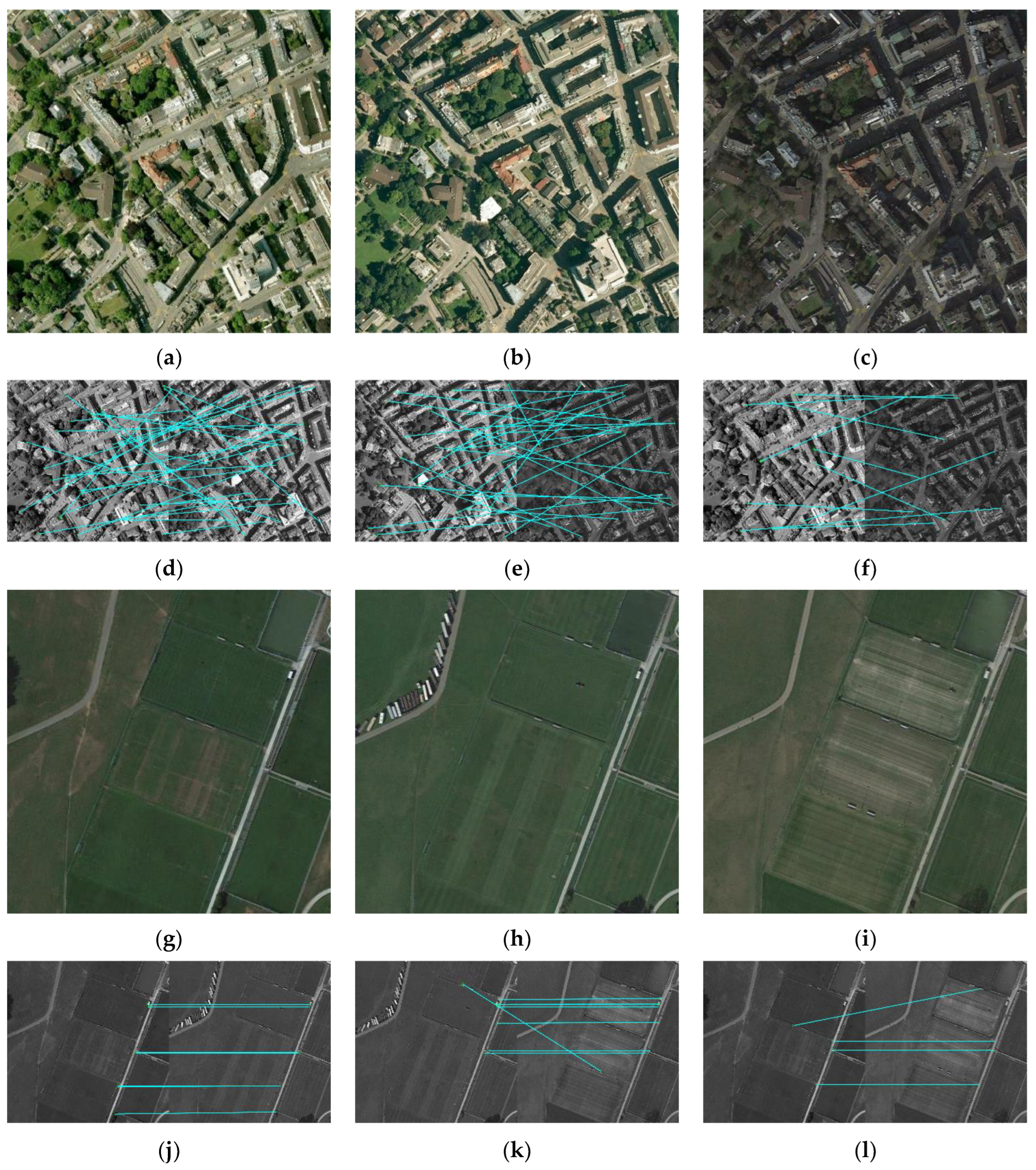
| Similarity | Image Pairs (with Buildings) | Image Pairs (Flat Area) | ||||
|---|---|---|---|---|---|---|
| (a,b) | (b,c) | (a,c) | (f,g) | (g,h) | (f,h) | |
| SURF features using FLANN (inliers/correspondences) | (0/29) | (1/28) | (0/10) | (7/7) | (7/8) | (3/4) |
| Correlation coefficients [16] | 0.17 | 0.24 | 0.26 | 0.64 | 0.47 | 0.56 |
| (18°, 45°) | (36°, 135°) | (54°, 225°) | (72°, 315°) | |
| OP Shadow Images of DSM (a) | 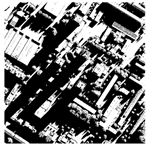 | 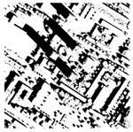 |  | 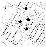 |
| OP Shadow Images of DSM (b) | 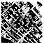 |  |  |  |
| Methods | Spectral Band or Color Space | Descriptions | Shortcomings |
|---|---|---|---|
| Mathematical based | |||
| Otsu [45] | Gray-level pictures | Calculating the maximum value between-class variance. | Unsatisfactory shadow detection results when the histogram is unimodal or the variance difference between shadow and non-shadow is large. |
| Tsai et al. [46] | HSI; YIQ color space | Applying Otsu’s [45] method on ratio map between hue and intensity in color space. | |
| Chung et al. [47] | HSI color space | Iterative thresholding algorithm in independent areas based on Tsai’s [46] method. | |
| Morphology-based | |||
| Nagao et al. [48] | R,G,B, Near Infrared (NIR) | Uses the value of grayscale at “first valley” as a threshold. | Fails if the histogram is unimodal. |
| Richter and Muller [49] | Hyperspectral image (better in short-wave infrared band) | Identifying threshold between “first valley” and main peak. | Restricted to cases with less than 25% of shadow pixels in the scene. |
| Chen et al. [50] | R, G, B, NIR | Similar to Nagao et al.’s [48] strategy under bimodal histogram conditions; using the position of the first peak as the decision surface to solve unimodal distribution. | Prone to under-detection when the histogram is unimodal. |
| Predicted Positive | Predicted Negative | ||
|---|---|---|---|
| Reference positive | TP | FN | |
| Reference negative | FP | TN | |
| Producer’s accuracy | User’s accuracy | Overall accuracy | F-score |
| Temporal Acquisitions | T1 | T2 | T3 | T4 | T5 | T6 |
|---|---|---|---|---|---|---|
| Date (yy/mm/dd) | 10/02/27 | 12/04/02 | 15/07/15 | 16/09/07 | 18/08/16 | 20/03/18 |
| Solar azimuth angle | 164.45 | 159.24 | 251.44 | 209.25 | 224.75 | 194.90 |
| Solar elevation angle | 33.12 | 46.03 | 44.89 | 44.88 | 48.73 | 40.99 |
| Method | Overall Accuracy | F-Score | Time Cost (s) |
|---|---|---|---|
| Otsu [45] | 66.69 | 65.25 | 0.019 |
| Tsai [46] | 85.88 | 76.23 | 0.198 |
| Xu et al. [54] | 90.35 | 85.61 | 0.022 |
| Chen et al. [50] | 88.47 | 83.30 | 0.097 |
| Proposed method | 91.56 | 86.96 | 0.038 |
| Navigation Model | RMSE(m) | Average RMSE (m) | |||||
|---|---|---|---|---|---|---|---|
| Ref1 (T1) | Ref2 (T2) | Ref3 (T3) | Ref4 (T4) | Ref5 (T5) | Ref6 (T6) | ||
| IMU | 95.95 | 95.95 | 95.95 | 95.95 | 95.95 | 95.95 | 95.95 |
| IbM | 19.10 | 16.58 | 42.09 | 13.41 | 14.40 | 17.15 | 20.45 |
| SbM | 10.31 | 10.31 | 10.31 | 10.31 | 10.31 | 10.31 | 10.31 |
| FM | 9.28 | 10.13 | 10.30 | 7.90 | 8.66 | 9.05 | 9.27 |
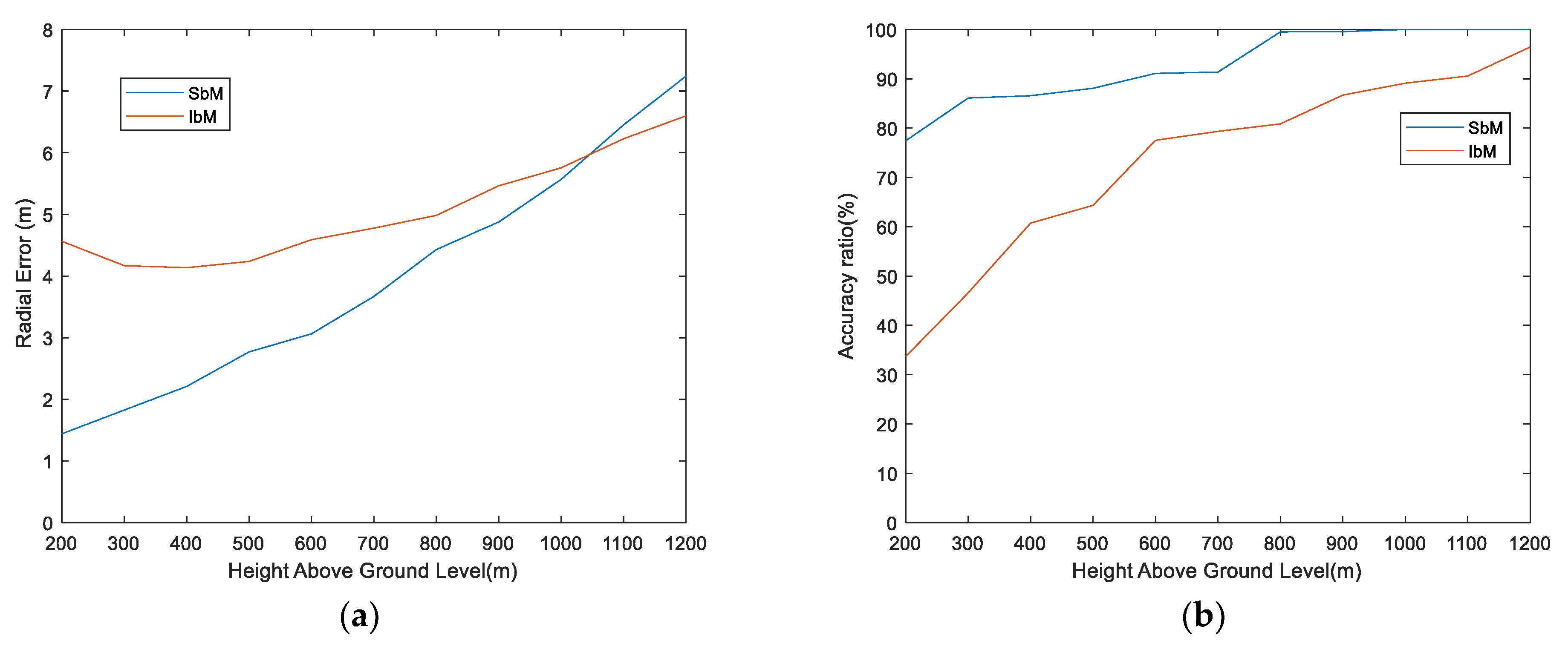
| Matching Model | Ref1 (T1) | Ref2 (T2) | Ref3 (T3) | Ref4 (T4) | Ref5 (T5) | Ref6 (T6) | Average Ratio (%) |
|---|---|---|---|---|---|---|---|
| IbM | 31 | 33 | 6 | 35 | 37 | 26 | 42.4% |
| SbM | 52 | 52 | 52 | 52 | 52 | 52 | 78.8% |
| FM | 53 | 54 | 52 | 57 | 59 | 55 | 83.3% |
| IbM (N) and SbM (P) | 22 | 21 | 46 | 22 | 22 | 29 | 40.9% |
| IbM (P) and SbM (N) | 1 | 2 | 0 | 5 | 7 | 3 | 4.5% |
| Matching Model | Ref1 (T1) | Ref2 (T2) | Ref3 (T3) | Ref4 (T4) | Ref5 (T5) | Ref6 (T6) | Total Average Radial Error (m) |
|---|---|---|---|---|---|---|---|
| IbM | 6.37 | 2.92 | 4.72 | 4.90 | 3.77 | 4.61 | 4.55 |
| SbM | 1.22 | 1.22 | 1.22 | 1.22 | 1.22 | 1.22 | 1.22 |
| Time (s) | IbM | SbM | ||
|---|---|---|---|---|
| Real-Time Intensity Image | Reference Intensity Map | Real-Time Shadow Image | Reference Shadow Map | |
| 121 |  |  |  |  |
| 151 |  |  |  |  |
| 171 | 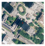 |  | 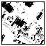 |  |
| 521 |  |  | 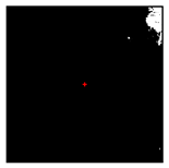 | 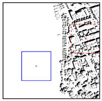 |
| 611 |  |  |  |  |
Publisher’s Note: MDPI stays neutral with regard to jurisdictional claims in published maps and institutional affiliations. |
© 2022 by the authors. Licensee MDPI, Basel, Switzerland. This article is an open access article distributed under the terms and conditions of the Creative Commons Attribution (CC BY) license (https://creativecommons.org/licenses/by/4.0/).
Share and Cite
Wang, H.; Cheng, Y.; Liu, N.; Zhao, Y.; Cheung-Wai Chan, J.; Li, Z. An Illumination-Invariant Shadow-Based Scene Matching Navigation Approach in Low-Altitude Flight. Remote Sens. 2022, 14, 3869. https://doi.org/10.3390/rs14163869
Wang H, Cheng Y, Liu N, Zhao Y, Cheung-Wai Chan J, Li Z. An Illumination-Invariant Shadow-Based Scene Matching Navigation Approach in Low-Altitude Flight. Remote Sensing. 2022; 14(16):3869. https://doi.org/10.3390/rs14163869
Chicago/Turabian StyleWang, Huaxia, Yongmei Cheng, Nan Liu, Yongqiang Zhao, Jonathan Cheung-Wai Chan, and Zhenwei Li. 2022. "An Illumination-Invariant Shadow-Based Scene Matching Navigation Approach in Low-Altitude Flight" Remote Sensing 14, no. 16: 3869. https://doi.org/10.3390/rs14163869
APA StyleWang, H., Cheng, Y., Liu, N., Zhao, Y., Cheung-Wai Chan, J., & Li, Z. (2022). An Illumination-Invariant Shadow-Based Scene Matching Navigation Approach in Low-Altitude Flight. Remote Sensing, 14(16), 3869. https://doi.org/10.3390/rs14163869