1. Introduction
The standing wood characteristics of trees provide important three-dimensional data [
1] that can be extracted to obtain detailed information, such as a tree’s position, height, wood volume, and diameter at breast height [
2]. While the information on standing characteristics is important for forest resource management [
3], field inventories [
4], and artificial afforestation, it can also assist in the research of tree animal habitats and their habitat structures [
5] and in urban gardens for landscape design [
6]. Traditional methods to obtain tree information generally require manual field measurements, and there are many tools and methods to measure forestry information directly [
7]. However, this process is highly time-consuming and may cause some damage to the trees. The development of modern remote sensing techniques, particularly light detection and ranging (LiDAR) sensor-based simultaneous localization and mapping (SLAM) [
8,
9,
10,
11], has made the exploration of imaging is gradually increasing [
12,
13] and has made it possible for technicians without considerable training to easily collect high-quality 3D information on forestry and reconstruct forestry point cloud maps. The laser scanning systems commonly used to collect forestry information can be divided into the following categories depending on the carrier platform: terrestrial laser scanning (including terrestrial laser, backpack laser, and vehicle-borne laser), satellite lidar scanning, and airborne laser scanning. Among them, terrestrial laser scanning systems are widely used in forest remote sensing because of their high flexibility and portability and good point cloud quality [
14,
15,
16,
17,
18]. The datasets we collected in this paper are based on terrestrial laser scanning. While the extraction of forestry 3D information has become increasingly rich and high quality, its complexity creates processing challenges.
Deep learning is currently one of the most widely researched areas of machine learning, with applications in object part segmentation, natural language processing, target detection, instance segmentation, semantic segmentation, and many other areas. Two-dimensional deep learning algorithms have been effectively used for the automatic classification of images and videos, such as the automatic recognition of whether fruit is corrupt for precision agriculture [
19], autonomous driving [
20,
21,
22], and town survey planning [
23]. While more of the representational information of 3D objects is reflected in point clouds, there have been many attempts to use deep learning on large 3D point clouds. For example, SnapNet [
24] converted a 3D point cloud into a set of virtual 2D RGBD snapshots, which could then be semantically segmented and projected onto the original point cloud data. SegCloud [
25] used 3D convolution on voxels and applied 3D fully convolutional neural networks to generate downsampled voxel labels. However, these methods do not capture the intrinsic structure of the 3D point cloud, and converting the point cloud to a 2D format also causes the loss of original information and spatial features. There are also methods for directly processing point clouds that have shown good performance. Point-Net [
26] was a pioneering work that used raw point clouds as deep learning inputs in each voxel, while PointNet++ [
27] built on PointNet with enhanced local structural information integration capabilities. These point cloud segmentation methods have many extensions and applications in forestry point cloud segmentation. For example, PointNet is used for the independent segmentation of tree crowns [
28], and PointNet++ is employed for the semantic segmentation of forestry environments [
29]. This paper focuses on the segmentation of tree point clouds (both stem and foliage) as we believe that good tree point cloud segmentation is a prerequisite for obtaining more accurate stand information.
Although all of the above methods have performed well in forestry point cloud se-mantic segmentation, the semantic segmentation of tree point clouds in artificial forestry scenarios still faces many challenges, one of which is the mismatch of point cloud geo-metric features in the scene. In an artificial forest environment where tree trunks are mainly characterized by linearity and verticality, tree crowns are mainly characterized by linearity and scattering, the ground is mainly characterized by planarity, and the number of point clouds for each geometric feature does not match the scene, making the network unable to learn the features of each label better. For example, the different numbers of planarity and vertical feature point clouds of branches affect the network’s learning of stem labels. The network does not learn enough about the rest of the geometric features, which affects segmentation when there are too many point clouds of one geometric feature. At the same time, as forestry point clouds are characterized by their large scale and disorder, it is difficult to achieve the same results on forestry point clouds with some convolution methods that work well in indoor environments. However, the energy partitioning proposed by [
30,
31] can partition largescale forestry point clouds into geometric partitions unsupervised, and then our proposed geometric feature balance model (GFBM) is employed to balance the overall geometric features and finally embed PointCNN [
32] for feature learning. PointCNN can preserve the spatial location information of point clouds due to the introduction of X-Conv, which can solve the problem of disorder in forestry point clouds to a certain extent.
In the context of previous studies, extracting tree parameters directly using commercial software is possible but does not exclude the rest of the point cloud in the environment [
17]. The Fully Convolutional Neural Network (FCN) series of networks can also be used to classify foliage and stem point clouds, but the results are mediocre [
33]. Our paper presents a method based on deep learning for extracting tree feature parameters from artificially planted forest. It removes distracting points from the environment by semantic segmentation and has good segmentation accuracy. It focuses on the following key points: (1) Energy segmentation partitions the original point cloud into geometric partitions; (2) Geometric feature matching balances the geometric features of the whole scene; (3) The geometrically balanced point clouds are embedded in the PointCNN network for learning; (4) The software 3D Forest [
34] and TreeQSM [
35,
36,
37,
38] are used to build a quantitative structure model (QSM) and then obtain standing tree characteristics, such as tree height and diameter at breast height.
3. Methods
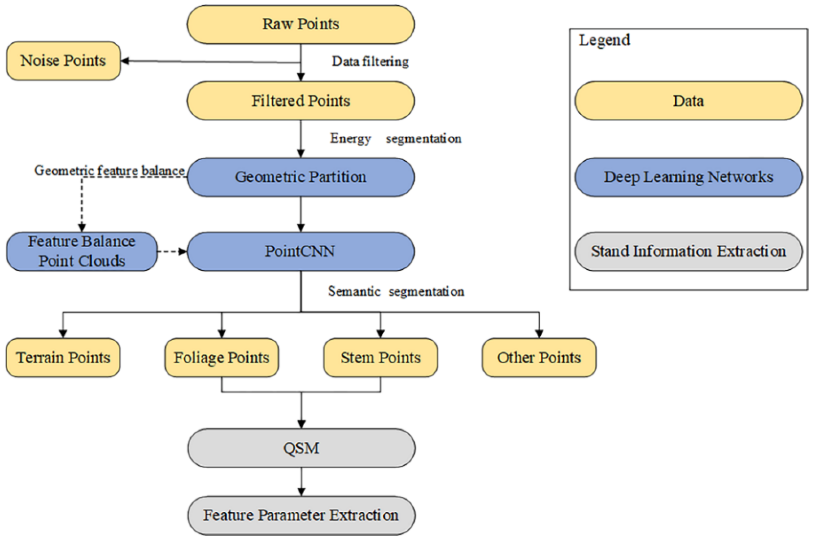
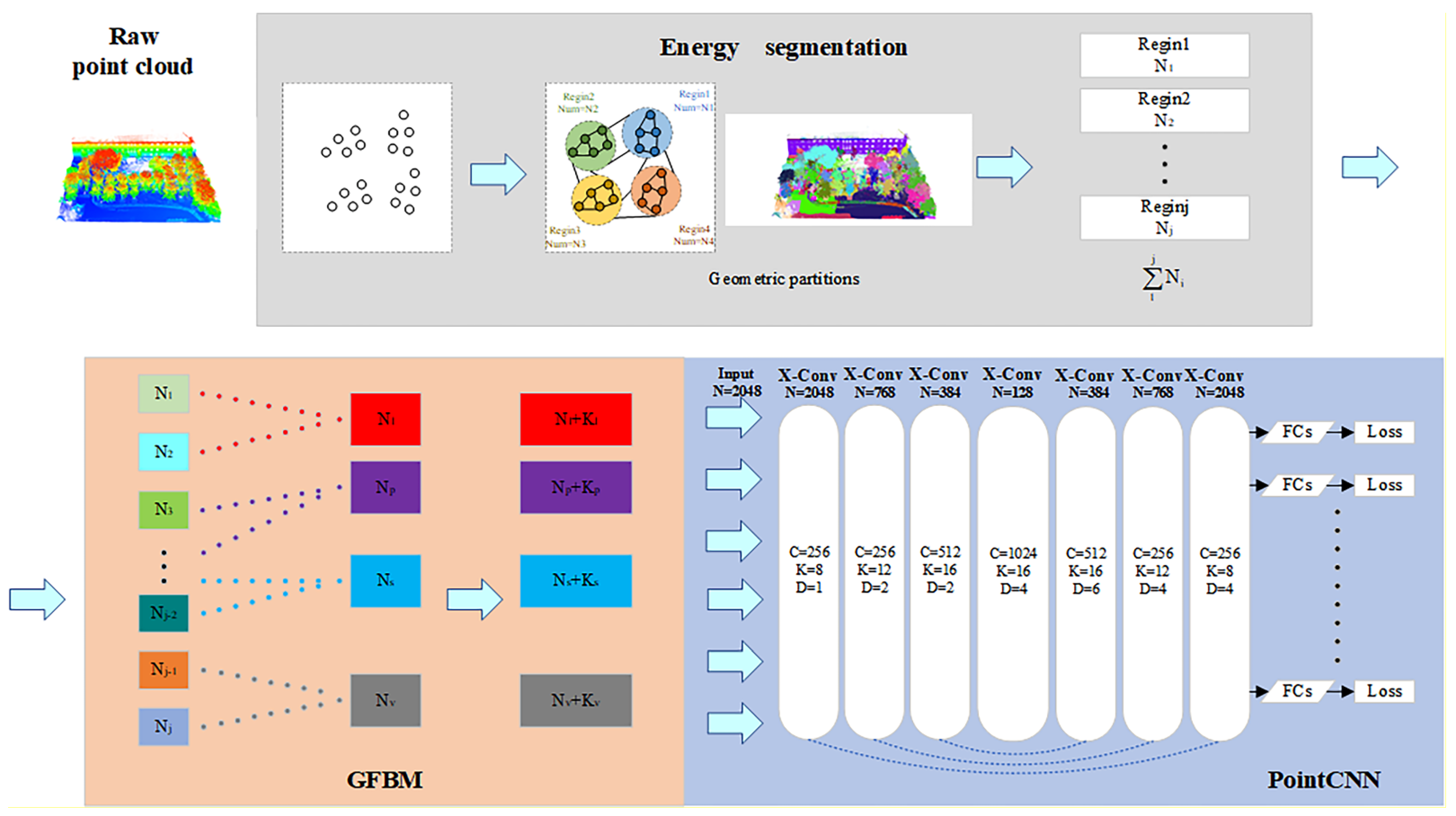
The deep learning framework we used in this work was based on energy segmentation, our proposed geometric feature balance model (GFBM), and PointCNN, as shown in
Figure 6. The energy segmentation function was used as a pre-segmentation framework for point clouds, allowing point clouds to be efficiently segmented into smaller geometric partitions based on object geometry without losing major fine details, and its energy segmentation method for forming geometric partitions is mainly listed here. Each geometric partition matched the geometric features after entering the GFBM so that the geometric features of the whole scene were balanced. A PointCNN based on TensorFlow [
43] was embedded in the subsequent semantic segmentation using a convolutional network to learn the input point cloud features.
3.1. Energy Segmentation Network
We describe the process of energy segmentation network in this section, where the input raw point cloud was computationally energy segmented, allowing the transformation of raw input point cloud data of millions of points into a few hundred geometric partitions, where the local geometry of the points within each partition was similar.
For the input point cloud P, the geometric partitioning was calculated based on the features of its 3D geometry. The point cloud was geometrically partitioned according to the above four features: linearity, planarity, scattering, and verticality. Each point will only belong to one geometric partition.
According to [
44], these features were defined by the local domain of each point in the point cloud. The eigenvalues for each point
λ1 ≥
λ2 ≥
λ3 were calculated of the covariance matrix of the positions of the neighbors. The neighborhood size was chosen such that it minimized the eigentropy E of the vector (
λ1/Λ,
λ2/Λ,
λ3/Λ), where E represents the point cloud adjacency relationship. According to the best neighbor principle proposed by Weinmann et al. [
44],
, which is in accordance with the optimal adjacency:
According to the findings of [
45], a formula for the linearity, planarity, and scattering of the local neighborhood can be presented based on these eigenvalues.
Linearity describes how elongated the neighborhood is, planarity describes how well it is fitted by a plane, and high-scattering values correspond to an isotropic and spherical neighborhood. These three characteristics combine to form dimensionality. Verticality can also be obtained from the definition of eigenvectors and the values defined above. Let μ
1, μ
2, μ
3 be the three eigenvectors associated with, respectively,
λ1,
λ2,
λ3. We then define the unary vector of principal direction in R
3 as the sum of the absolute values of the coordinate of the eigenvectors weighted by their eigenvalues.
We considered that the vertical part of this vector characterizes the verticality of a point field.
In this article, the generalized minimal partition problem was studied by referring to the partition problem of global properties. For each point
i, we computed a vector of geometrical features and associated its local geometric feature vector f
i ∈ R
4 (dimensionality and verticality) to calculate piecewise constant approximation g*, where g* is defined as the vector of R
4×P minimizing the following Potts segmentation energy. We obtained the point cloud geometric partition by solving this optimization problem.
In the above equation, [ ] is an Iverson bracket; for any point
i belonging to
P,
is the regularization factor and influences the coarseness of the partition; ω
i,j is the edge weight, equal to 0 in 0 and 1 everywhere else. For the partition, l
0-cut pursuit [
46] was used to solve this energy partitioning problem. The advantage of this method is that it does not require the definition of the size of the point cloud and the different energy partitions of the whole scene are obtained quickly after calculation.
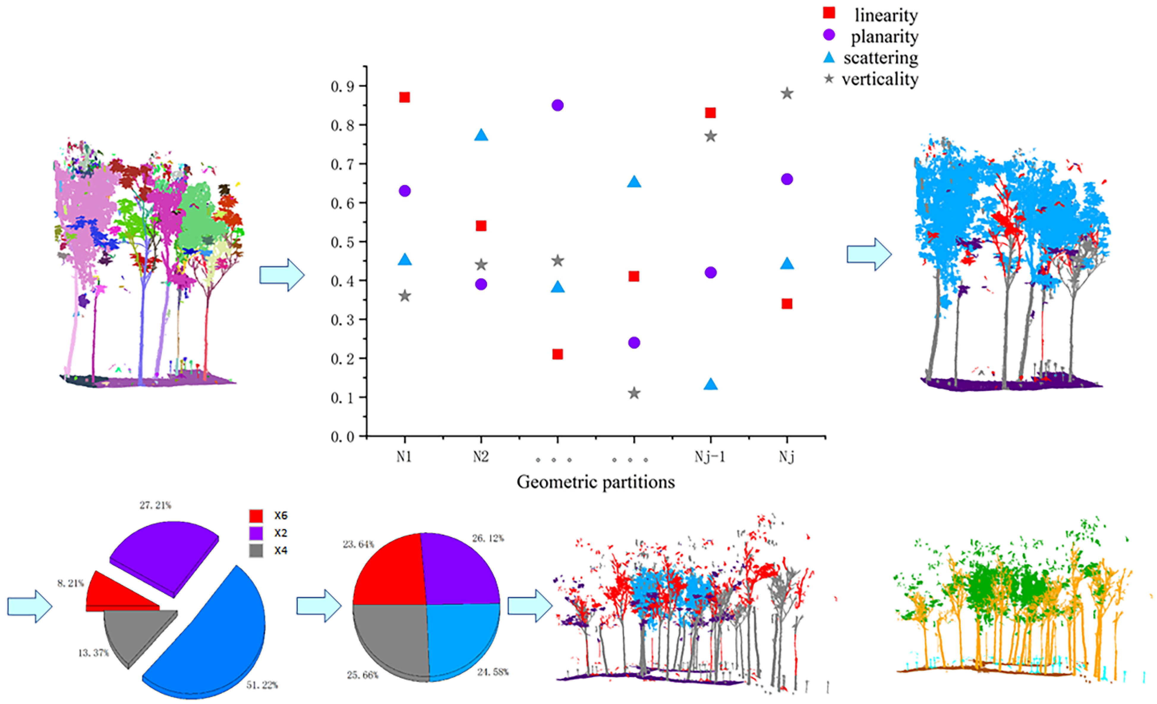
3.2. Geometric Feature Balance Model
The main function of this module is to balance the geometric features of the point cloud input to the network. For example, for the trees in the point cloud, most of the branches have scattering geometric features predominantly, but there are also branches with more vertical or planarity geometric features, and increasing the number of these branches in the training set is beneficial to enhance the network’s learning of the details of the stem label. In this paper, the geometric features of the whole scene are balanced in-stead of a particular label, which is beneficial for global features and less computationally intensive. The overall process is shown in
Figure 7.
The formula for calculating the four geometric features of the local neighborhood was shown in the previous
Section 3.1. For each geometric partition, the average value of its four geometric features was calculated separately, and then the most representative feature of each geometric partition was selected as the geometric feature of this partition so that the number of point clouds with the four features as the main features in the whole scene could be obtained, respectively.
After the above operation, we obtained four types of point clouds with linearity, planarity, scattering, and verticality as the main features, namely, Pl, Pp, Ps, and Pv. The geometric feature balancing strategy was to use the largest number of point clouds in the four-point cloud feature sets as the quantitative benchmark, and the rest of the geometric feature sets were aligned by this benchmark in order of magnitude, as shown in Equations (7)–(9) below. The geometric features were balanced by copying and panning the point cloud, adding a random angle of rotation to the panning to increase the generalizability of the network. Meanwhile, to ensure that the overall geometric features of the scene do not change as a result of the rotation operation, the rotation was performed with a reference axis paired with Z.
3.3. PointCNN Deep Learning Network
PointCNN solves the point cloud disorder problem by employing transpose matrices. Compared to PointNet, which uses symmetric functions to deal with point cloud disorder, PointCNN can reduce feature loss. In PointCNN, we used an encoder–decoder paradigm, it is called X-conv, where the encoder reduces the number of points while increasing the number of channels. Then, the decoder part of the network increases the number of points, and the number of channels is incrementally reduced. The network also uses the same “skip connection” architecture as U-Net [
47]. The most important characteristic of X-conv is that it can both weight and guarantee the invariance of the input features, and then apply the traditional convolution to the features, it is the basic block of PointCNN.
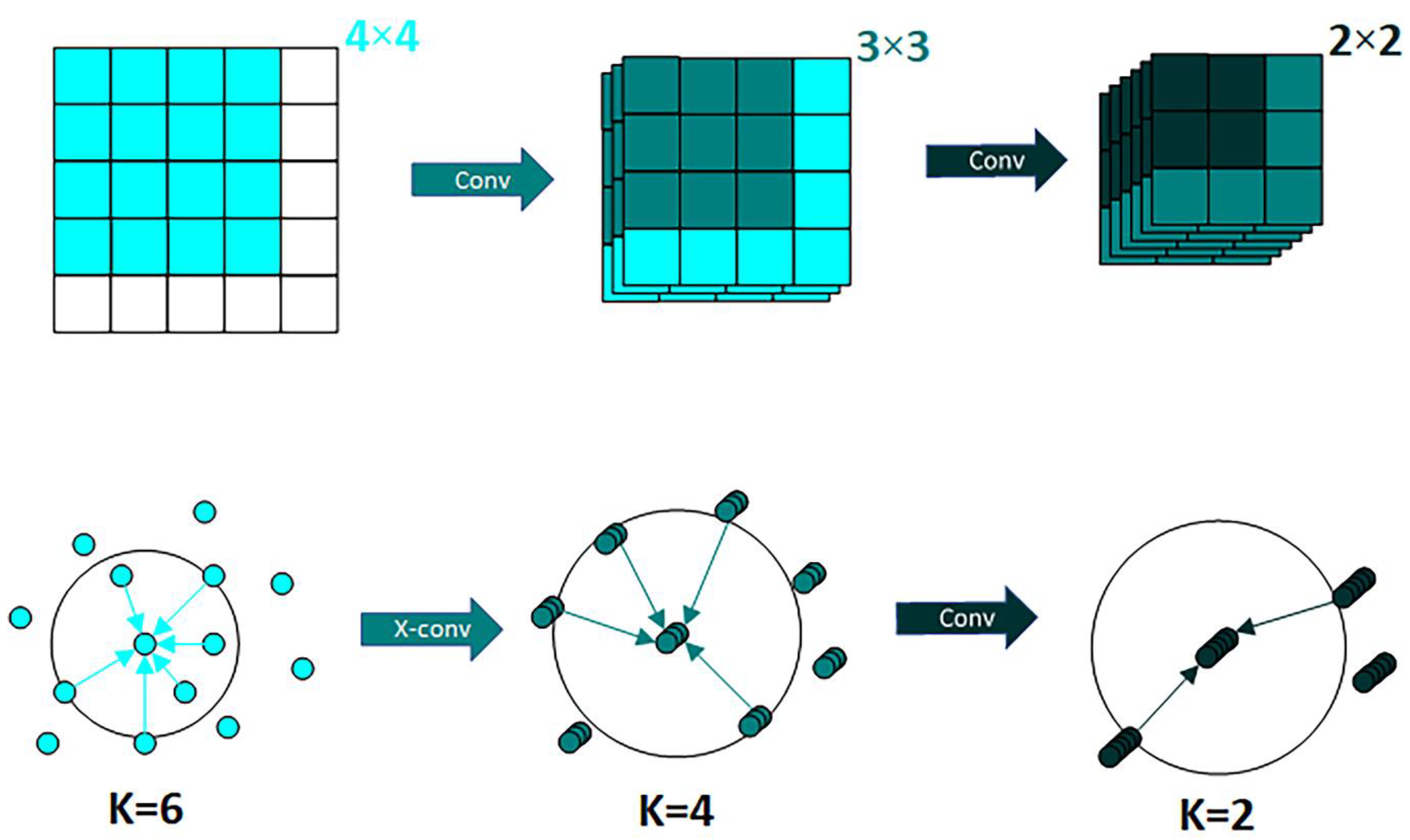
PointCNN differs from traditional grid-based CNNs in two main ways. First, the method of local region extraction is different. While CNN extracts local features directly through K × K blocks, PointCNN extracts local features by representing K neighboring points on a point and then fusing the features in the K neighborhood by weighting the sum, enabling it to achieve the same effect as a convolution operator fusing domain features in regular data. Second, the method of local region information learning is also different. CNN usually extracts image features by Conv and then pools downsampling, while PointCNN uses X-Conv to extract features, aggregating them into fewer points to increase the channels to recursively learn the correlation with the surrounding points. A comparison of the two methods is shown in
Figure 8.
3.4. Training Details and Performance Measures
We provide more details of the training in this section. All training and testing were conducted on a personal computer, with CUDA-accelerated computation using an Nvidia 3060 GPU during the training process. A development environment of Python 3.6 and TensorFlow GPU 2.4.1 was set up on Ubuntu 18.04, with a basic learning rate of 0.0002 and batch study size of 8. The network was trained over 150 rounds, and all were trained using a randomized dropout method, which was applied before the last fully connected layer to reduce over-fitting. This method can effectively improve the generalization of the training process and make the algorithm perform well on sparse point clouds.
A comparison between the manually measured real values and the QSM measurements was carried out as a reference for the effectiveness of standing wood feature information extraction. The Softmax cross-entropy function was used as the loss function of the deep learning network. To evaluate the performance of the semantic segmentation model, Python packages Numpy and Seaborn were used to evaluate our results and generate confusion matrices.
IoU is the evaluation index for each category, and
OA is the overall precision evaluation index of the dataset. Precision indicates the proportion of actual positives to predicted positives and Recall indicates the proportion of actual positives that are correctly predicted.
where
TP is the true positive,
TN is the true negative,
FP is the false positive, and
FN is the false negative.
3.5. QSM Formation and Feature Parameter Extraction
The QSM of a tree is the structural model of the tree, describing its basic branch structure and geometric and volumetric properties. These properties also include the total number of branches of the tree and the parent–child relationship of the branches, the length, volume, and angle of individual branches, and the branch size distribution. There are other properties and distributions that can be easily calculated from the QSM. The QSM consists of construction blocks, usually of some geometric shape, such as cylinders and cones. The cylinder was used here as it is the most reliable and is highly accurate for estimating diameters, lengths, orientations, angles, and volumes in most situations. A QSM consisting of cylinders provides a downsampled representation of the tree and can store a lot of information about the tree, as mentioned previously.
In actual cases, using the semantically segmented tree point cloud followed by QSM and standing wood feature information extraction can reduce the interference of the rest of the point cloud in the environment on the accuracy of the tree information and also prove the necessity and accuracy of our point cloud segmentation method.
In this paper, 3D Forest software was used to instance segment the semantic segmented tree point clouds, and then TreeQSM was used to extract standing wood feature information from our segmented point clouds by fitting columns to convert the point clouds into QSM models, which can represent over 99% of our segmented tree trunk point clouds with an accuracy of over sub-millimeter. TreeQSM has two key steps in extracting tree parameters; the first step is the topological reconstruction of branching structure, which is the segmentation of the point cloud into stem and individual branches. The second step is the geometrical reconstruction of branch surfaces, which is realized by fitting cylinders. For more details on the original TreeQSM method, please refer to the original articles [
35,
36,
37,
38].
4. Results
The segmentation results for the two test datasets are shown here, including the energy segmentation results, the semantic segmentation results, and the results of standing wood feature parameter extraction for the processed tree point clouds.
4.1. Semantic Segmentation Results
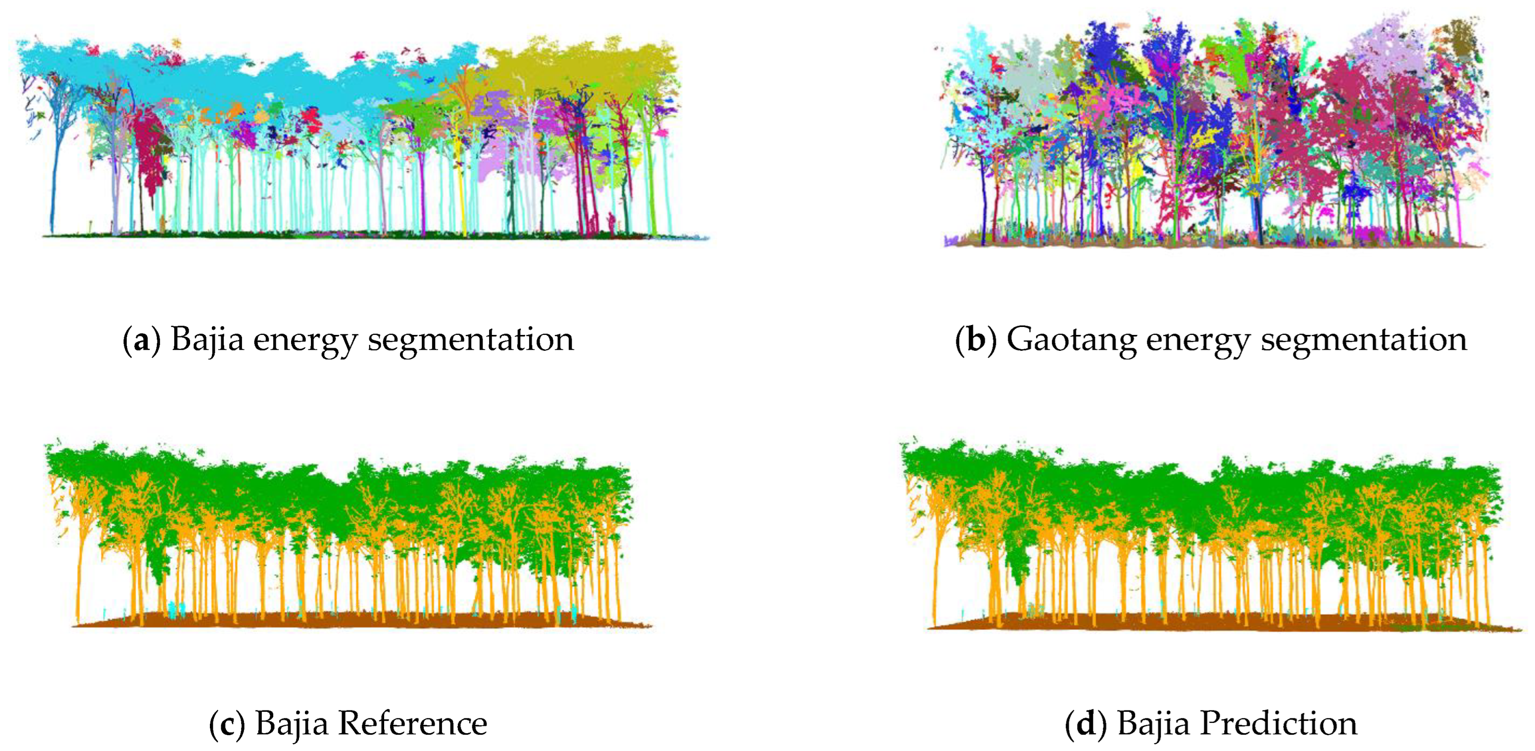
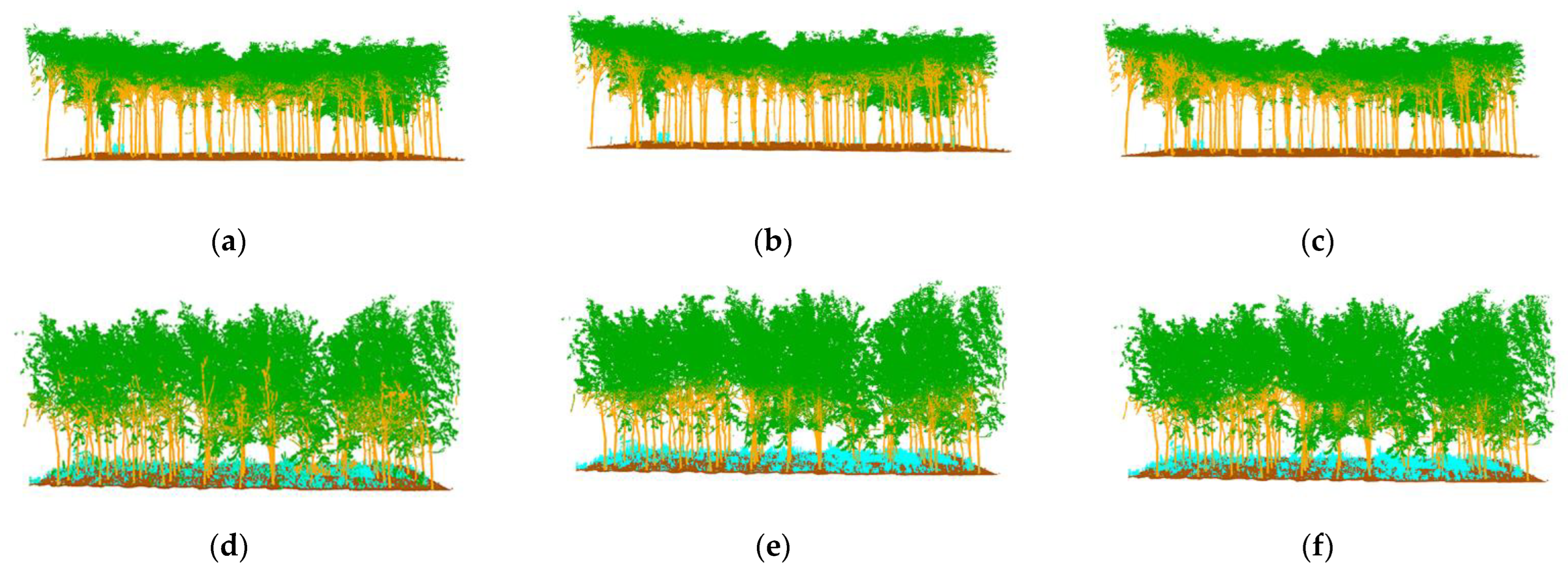
The energy partitioning results for the test set are shown in
Figure 9a,b, where the left-hand side shows the partitioning results for the Bajia dataset and the right-hand side shows the partitioning results for the Gaotang dataset. It can be seen that the morphology of the poplar and Tsubaki trees in the two datasets are completely different; the Gaotang dataset that has more branches and leaves has significantly more geometric partitioning. Due to the disorderly nature of the point cloud, the energy partitioning of the test set does not affect the final result of the semantic partitioning and is only shown here to demonstrate the process of unsupervised segmentation.
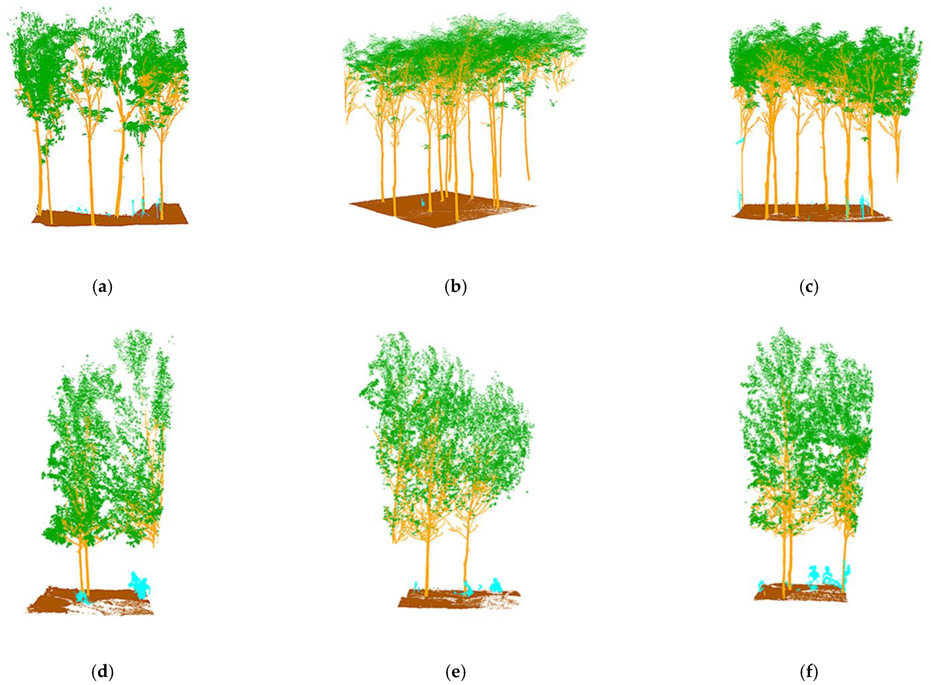
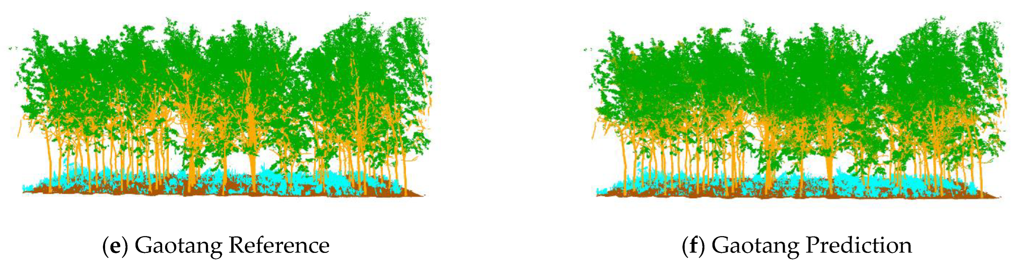
The semantic segmentation results are shown in
Figure 9c–f, with the manually annotated point clouds on the left and the segmented point clouds on the right, which are the result of energy segmentation into geometric partitions followed by semantic segmentation. These point cloud inspection sets are visually very similar to the reference data for manual segmentation. For the segmentation results, the tree point cloud is well-segmented from the whole point cloud. While some stems and foliage are misclassified into ground and other points, and some ground is misclassified into foliage, which is not common. In the Bajia test set, a small number of points of trees are misclassified as ground, which occurs in point clouds located at the edges of the data sample and in the Gaotang dataset. While some of the shrubs in the other point categories are misclassified as stems mainly in the root point cloud, the number of misclassifications is not significant.
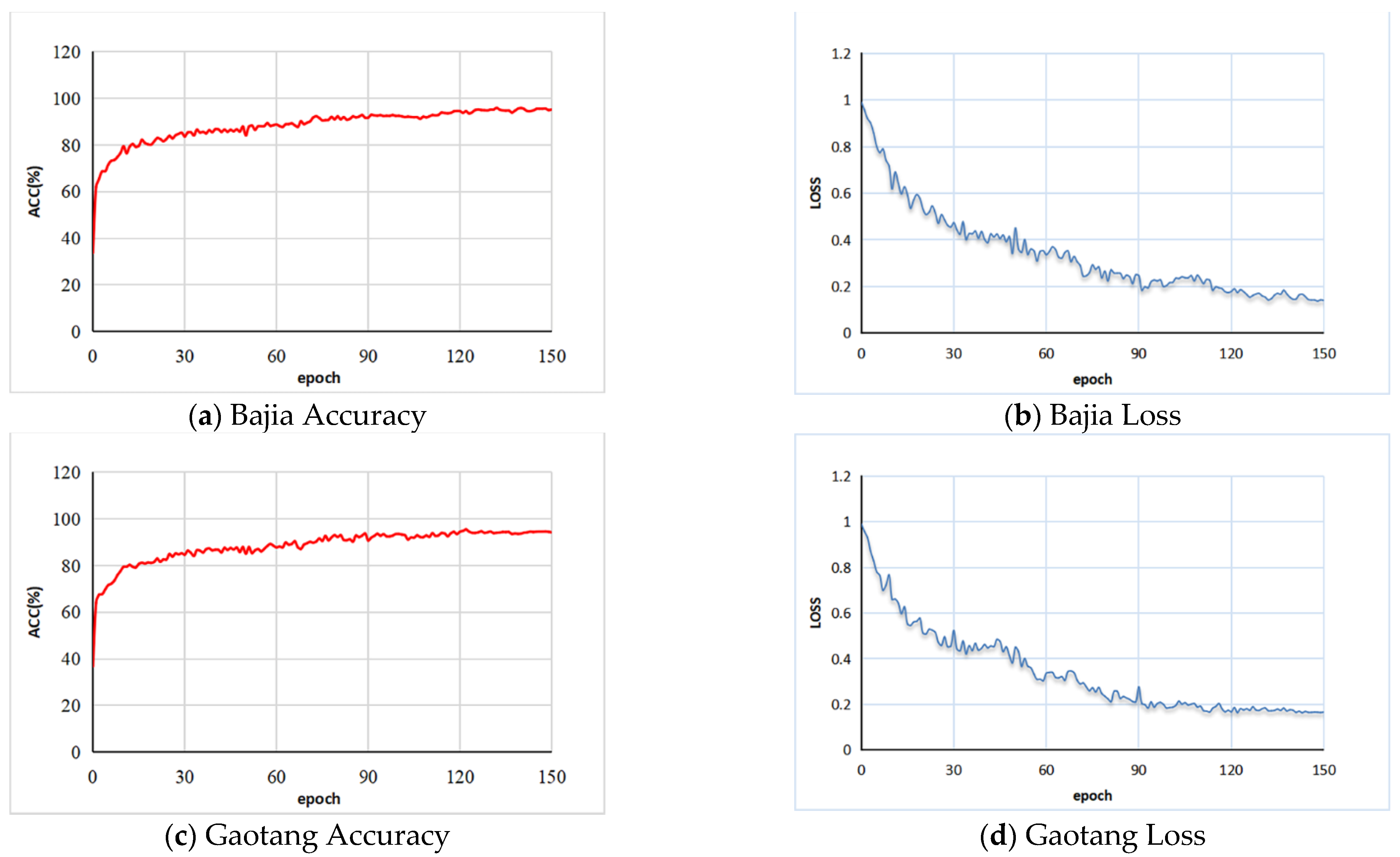
The training accuracy and loss curves during the training process of the Bajia and Gaotang data sets are shown in
Figure 10. In the training process, the training accuracy tends to increase while the training loss function tends to decrease, which indicates that our network has a good learning ability for global features. For the Bajia dataset, the total training and validation time is approximately 120 h. Additionally, for the Gaotang dataset, the total training and validation time is approximately 110 h. After 130 rounds of training, the training accuracy and loss curve stabilize in the Bajia dataset, with the training accuracy and loss function converging to 0.95 and 0.14, respectively, and in the Gaotang dataset, these figures are closer to 0.93 and 0.18, respectively.
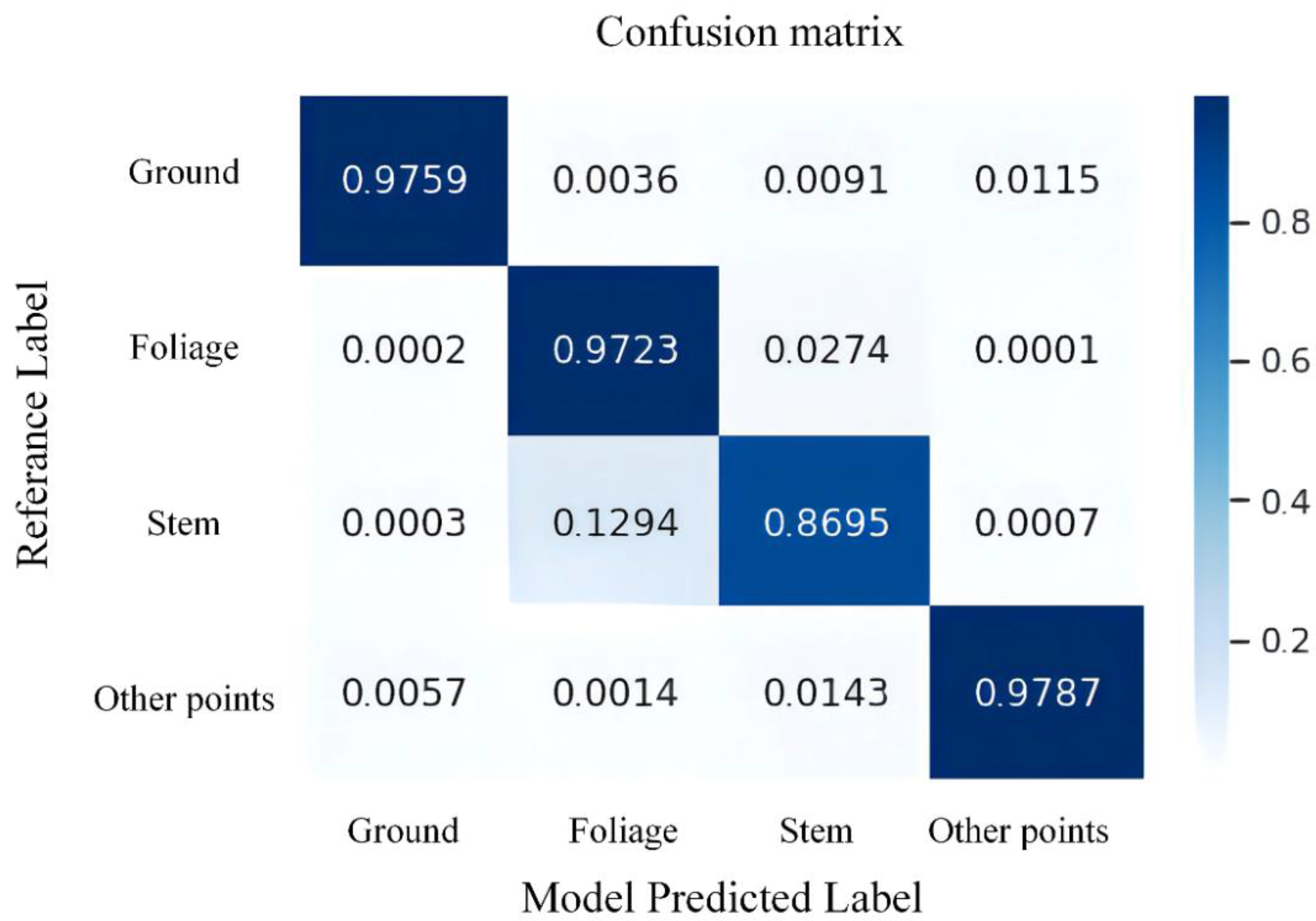
For the Bajia and Gaotang datasets, the segmentation results achieve our goal of data processing, and the tree point cloud is well-segmented from the overall point cloud. Of the four labels, we observed that for the three categories of ground, foliage, and other points, the model has significantly higher accuracy than the stem label when predicting and that the other point category with the fewest points in the entire map has the highest precision. This is illustrated in
Figure 11, which shows the semantic partitioning confusion matrix for the overall two test sets.
In both test datasets, the overall accuracy of trees (including stem and foliage) in the Bajia dataset is 0.94, significantly higher than the 0.90 of the Gaotang dataset. This may be because the leaves of the Tsubaki trees in the Bajia dataset are mainly concentrated at the top of the trees, and the branch angle is large, so the leaf feature network is easier to learn. In contrast, the triploid poplar planted in the Gaotang dataset has a large number of branches and a large branch-to-diameter ratio, the tree canopy envelope is tighter, the leaves are smaller and more numerous, and there are a large number of ground plants that affect the segmentation accuracy of the tree point cloud and cause the trunk to be misclassified into leaves more often.
In these two datasets, the ground class had the highest Recall, reaching 0.983 and 0.988, respectively. The other classes have high Precision but low Recall in the Bajia dataset, probably because the other point classes contain several types of unappreciated points, including light-emitting instruments and human shadows. As these objects are more different and less numerous in the overall point cloud map, their features are not well learned by the network, which leads to their misclassification as stems. The detailed metric parameters are shown in
Table 2.
4.2. Comparison of QSM Results with Manual Measurements
The segmented point cloud was used to generate a QSM model using 3D Forest software and MATLAB-based TreeQSM and then extracted to analyze the tree feature information, which was an important step in our overall workflow. Semantic segmentation was carried out to prepare for the extraction of stand information to deal with the interference of distracting objects in the artificially planted woods on the extraction of tree feature information.
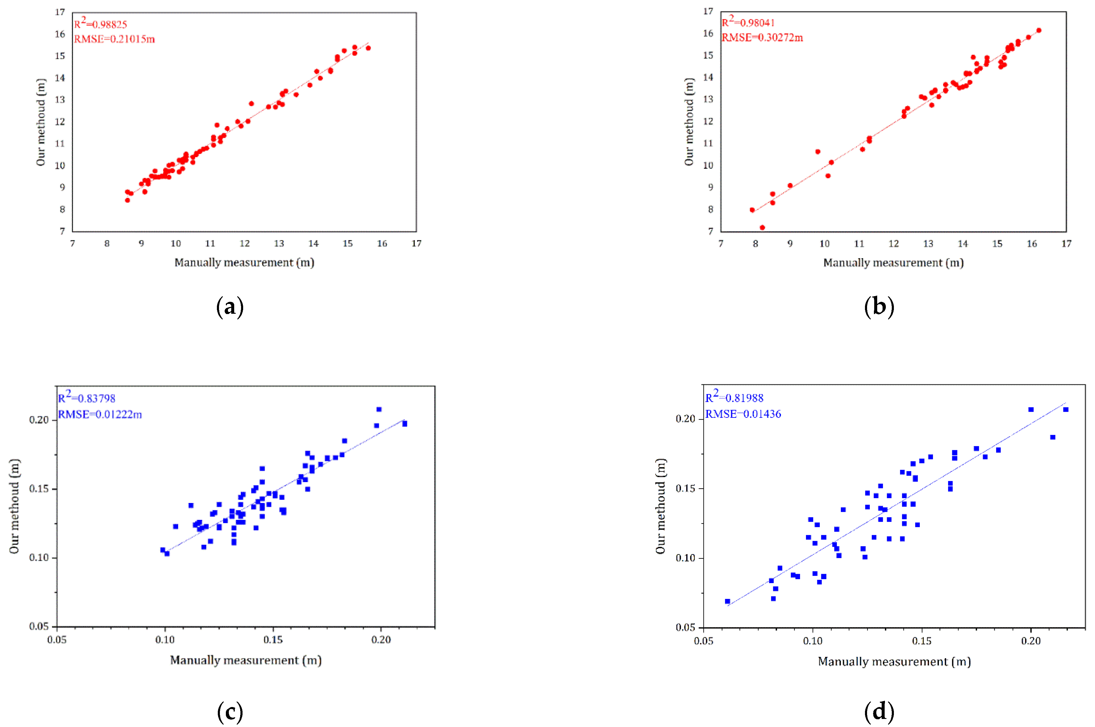
A brief demonstration of the extracted tree height and diameter at breast height data and its comparison with the actual measurements after forming the QSM model for the test dataset is shown in
Figure 12. The correlation coefficient
R2 and the root-mean-square error were calculated separately for both datasets to qualitatively evaluate our results.
As shown in
Figure 12, a total of 74 trees from the Bajia dataset and 57 trees in the Gaotang dataset were counted for both height and diameter at breast height compared to the manual measurements. It can be seen that the accuracy of both height and diameter at breast height is higher in the Bajia dataset, likely because the branches of the Tsubaki tree branch are at large angles and cross over less, and the diameter at breast height is relatively larger.
In both datasets, the accuracy of tree height seems better than diameter at breast height, the point clouds of the trees are fitted frame by frame, and some deviations may occur during the fitting process, but this is acceptable and the QSM algorithm still does not fit the diameter at breast height well enough, increasing the measurement error. The results of the standing wood information extraction achieved by QSM are briefly presented here, illustrating the importance and effectiveness of the semantic segmentation work in this paper.
5. Discussion
5.1. Evaluation of Our Approach
Extracting information on standing tree characteristics in forestry environments through LiDAR scanning techniques is of great importance for forestry automation. Analyzing the physical parameters of trees can be very helpful for studying the relationship between the standing canopy and sap flow, light, soil, etc. Our approach provides a new method to reliably extract tree feature information from TLS point clouds of artificially planted woods. The automatic extraction of tree point clouds from laser scanned data is an important prerequisite for standing feature information extraction, tree phenotype, and biophysical parameter estimation. The semantic segmentation method in this paper provides a new and reliable method for extracting tree point clouds from LiDAR-scanned forestry point clouds. This semantic segmentation method enhances the learning of the network for artificially planted woodland object features by balancing the geometric features in the scene, and the point clouds are segmented by PointCNN. The semantic segmentation in both forestry scenes obtains good segmentation results, and this method has high robustness.
However, there are still some limitations to this work. For example, the manual labeling of point clouds remains highly subjective. While the ground and other points are generally correctly labeled, when labeling tree stem and foliage, although the majority of points are labeled accurately, a small number of points are inevitably incorrectly labeled due to the limited time available and the fact that some of the blurred points are difficult to distinguish manually. In
Section 2.4.1, we also showed the scale of our labeling of point cloud categories, where the fuzzy stem-like point clouds are labeled as foliage-like so that the network can learn the features of the complete stem point cloud to the maximum ex-tent and better segment the stem point cloud from the overall point cloud. We believe that the obtained overall segmentation accuracy of 0.9 for the tree point cloud achieves our de-sired goal. According to our segmentation study on the two datasets, the accuracy of tree segmentation in the Bajia dataset is 4% higher than that in the Gaotang dataset. The main reason for this phenomenon may be the fact that the physical parameters of the Tsubaki tree in the Bajia dataset are completely different from those of the triploid aspen in the Gaotang dataset. The Tsubaki tree has an oblate crown with many branches, and the leaves are relatively large, whereas the long branch leaves of the triploid hairy poplar are broadly ovate or triangular–ovate leaf-shaped and relatively small.
Additional results are also significant. For example, in the Bajia dataset, some tree point clouds on the upper boundary of the point cloud edge are misclassified as ground class, although the number of misclassifications is very small, which may be due to the similarity between the point cloud boundary features and ground features. In the Gaotang dataset, leaves on branches are misclassified as stems, which may be due to the lack of de-tailed labeling or poor learning of network features. However, this does not have a negative impact on the extraction of standing tree information.
Overall, the method of extracting information from artificially planted woods explored in this paper effectively extracts standing tree feature information, and the semantic segmentation method maximizes the preservation of spatial features of the point cloud and achieves good performance in the final test. The network obtains optimal weights through iteration during the training process, making the model robust in identifying the point clouds that form the structure of tree trunks and leaves.
5.2. Comparison with Similar Methods
We also compared our experimental results with the results of other papers. It is worth noting that as different data and methods of labeling the data were employed, these values do not necessarily characterize the absolute performance of the algorithm, but still provide a certain reference for our research.
A comparison of our study with other papers can be seen in
Table 3, where the definitions of the classes are different in each paper, but essentially all contain two classes: leaves and trunk. In the above study, of the four classes counted, [
29] performs best in terms of overall accuracy, which employs a method based on PointNet++. By comparison, our method performs better in the ground and other point classes, with similar accuracy in the foliage and lower accuracy in the stem classes. In contrast, [
48] compares a variety of methods, applying a 3D convolutional neural network on voxels and PointNet to segment the dataset, and also compares data with intensity and without intensity, respectively. An overall accuracy of 0.925 was obtained in [
49], which used an approach based on unsupervised learning.
Although there are a number of limitations to our comparisons here, our method obtained more accurate results. This comparison provides a clear understanding of the differences between methods, which will remain a reference for our future research work.
We also compared different semantic segmentation methods on both the Bajia and Gaotang datasets using three algorithms, including the MVF CNN [
50] (which also uses CNNs), the point-based method PointNet, and the original unaltered PointCNN network.
MVF CNN is a deep learning-based multi-scale voxel and feature fusion algorithm for large-scale point cloud classification. First, the point cloud is transformed into two different-sized voxels. The voxels are then fed into a three-dimensional convolutional neural network (3D CNN) to extract features. Next, the output features are fed into a recommended global and local feature fusion classification network (GLNet), and the multi-scale features of the main branch are finally fused to obtain their classification results.
PointNet uses the input of the original point cloud to maximize the spatial characteristics of the point cloud, partitioning the input into voxels of uniform size. The input of the network is the 3D coordinates (n × 1024 × 3) of the three-dimensional point cloud containing n voxels and 1024 points within a voxel. This is then fed into the network for training.
PointCNN takes the structure from the original paper and does not change it, partitioning the input point cloud into uniformly sized voxels to feed into the network for training and prediction of the test set.
In this work, the network was trained, the test set was partitioned, and the maximum epoch was set to 200. The batch size used eight samples, and the learning rate was 0.0002. The segmentation results are shown in
Figure 13, and quantitative evaluations of the results are provided in
Table 4.
Among them, MVF CNN and PointNet show a similar accuracy of 0.85, and both methods have good accuracy in trunk and foliage classes. The original PointCNN has a higher accuracy of 0.91 compared to the previous two methods, and its stem precision is the best among the four methods. The overall accuracy of these three methods is not as good as our method. This suggests that our deep learning framework performs better in extracting spatial features of trees when processing point clouds of artificially planted trees captured by TLS.
5.3. Future Research Directions
In future work on this project, our focus will be on improving the accuracy of network segmentation. In practice, the higher the accuracy of the semantic segmentation, the less manual correction will be required, which will significantly reduce manual effort and facilitate the fully automated segmentation of the forest point cloud. We intend to increase the amount of data in the training set, add the manually corrected test set after segmentation to the training set, and iterate the training model again to enhance the recognition capability of the network. We will also explore the applicability of our method in different acquisition techniques, such as backpack radar and aerial radar. This will enable us to determine its applicability on point clouds collected by more devices, test its effectiveness in different forestry contexts, such as primary forest or urban greenery, and explore its segmentation effectiveness in larger contexts. The problem of shading between branches can affect the accuracy of manual labelling and the classification results of trees, just as shading can also have an impact on leaf area calculations [
51]. In future work, we will also consider how to address this issue, for example, by considering whether the use of aerial radar data [
52] would reduce this effect or by considering some graph-based deep learning networks [
53].
We will also explore the effectiveness of different neural networks for segmenting point clouds of artificially planted trees in future work. The varied results of the two datasets in this paper indicate that different tree species may behave differently on the same network when using the same tree feature information extraction method, thus whether different neural networks are suitable for different tree species point cloud data. Exploring whether there is a relationship between the choice of neural network and the ability to segment tree point clouds in a forestry environment is of great significance for establishing a fully automated method for extracting stand information.
6. Conclusions
This work aimed to obtain a complete ground-based radar point cloud tree information extraction method of artificially planted trees to help us to better investigate the relationship between the 3D physical information of trees, tree growth, and tree cultivation practices. We divided the work into forestry point cloud map building, deep learning-based semantic segmentation, and QSM-based tree feature information extraction.
The forestry map was built using RIEGL equipment and this paper focused on our proposed semantic segmentation method based on deep learning as the forestry point cloud collected by LiDAR has noise, and point clouds of other objects are not relevant. Semantic segmentation is an extremely important component for excluding the influence of other point clouds on the tree point cloud. Although the need for extracting tree point clouds in some practical applications can also be solved by direct manual segmentation, as human energy is limited and the forestry environment has a vast volume of data, semantic segmentation based on deep learning is undoubtedly the best approach. The point clouds are then processed using existing QSM methods to effectively obtain information on the standing wood features of the target.
Our method showed good segmentation results on the dataset, with RMSEs of 0.30272 and 0.21015 m for tree height and 0.01436 and 0.01222 m for diameter at breast height in both datasets, respectively, with a high overall accuracy of 0.95 for semantic segmentation and 0.93 for trees. Compared to the manual segmentation of point clouds, our method has considerable advantages as an automated process for extracting feature information from artificial woodland point clouds collected by TLS, providing a strong foundation for creating a fully automated and high-precision method for extracting information from artificial woodland stands.


