Supervised Machine Learning Algorithms for Ground Motion Time Series Classification from InSAR Data

Abstract

The increasing availability of Synthetic Aperture Radar (SAR) images facilitates the generation of rich Differential Interferometric SAR (DInSAR) data. Temporal analysis of DInSAR products, and in particular deformation Time Series (TS), enables advanced investigations for ground deformation identification. Machine Learning algorithms offer efficient tools for classifying large volumes of data. In this study, we train supervised Machine Learning models using 5000 reference samples of three datasets to classify DInSAR TS in five deformation trends: Stable, Linear, Quadratic, Bilinear, and Phase Unwrapping Error. General statistics and advanced features are also computed from TS to assess the classification performance. The proposed methods reported accuracy values greater than 0.90, whereas the customized features significantly increased the performance. Besides, the importance of customized features was analysed in order to identify the most effective features in TS classification. The proposed models were also tested on 15000 unlabelled data and compared to a model-based method to validate their reliability. Random Forest and Extreme Gradient Boosting could accurately classify reference samples and positively assign correct labels to random samples. This study indicates the efficiency of Machine Learning models in the classification and management of DInSAR TSs, along with shortcomings of the proposed models in classification of nonmoving targets (i.e., false alarm rate) and a decreasing accuracy for shorter TS.

1. Introduction

Ground deformation is the consequence of physical events caused by natural or human activities, which can be analysed to provide the status of natural and anthropic hazards. Remote Sensing (RS) supplies tools to explore the temporal and spatial distribution in ground deformation. In May 2022, the European Ground Motion Service (EGMS) published the ground displacements of Europe [1,2], derived using Differential Interferometric SAR (DInSAR) techniques. The EGMS will make use of both Persistent Scatterers (PS) and Distributed Scatterers (DS). The EGMS consists of huge datasets of measurement points, thus appropriate procedures are required to manage such a large volume of information and to extract valuable outcomes.

Ground displacement classification has been proposed to categorize targets based on their Time Series (TS). For instance, a procedure was proposed by Cigna et al. (2011) [3] using the changes in the intensity of deformation velocities. Then, Berti et al. (2013) [4] presented six trends of ground displacements (stable, linear, quadratic, bilinear, discontinuous with constant velocity, and discontinuous with variable velocity). This approach has been recently improved to include TS affected by Phase Unwrapping Error (PUE) [5]. TS have also been categorized to detect accelerations and decelerations of TS related to landslides and slope failures [6,7].

Machine Learning (ML) classification/clustering approaches are able to improve the management of big geodata [8] and the accuracy of ground deformation classification [9]. Supervised and unsupervised learning approaches have been the main techniques employed in classification/clustering using Earth observation images. Supervised learning classifies and predicts data based on the characteristics of predefined classes, whereas unsupervised learning is based on algorithms that investigate similarities within the data to categorize them into the most similar clusters. Supervised algorithms have been widely employed to map input data using in situ reference samples. K-Nearest Neighbours, Random Forest (RF), Support Vector Machine (SVM), and different types of Deep Learning (DL) algorithms (e.g., Convolution Neural Network (CNN) and autoencoders) have been the most popular techniques in supervised classification. Various studies have investigated the potential of these algorithms in applications of InSAR TS, such as land subsidence [10] and landslide risk assessment [11], landslide detection [9,12,13], land subsidence prediction [14,15,16], fault slip [17], land subsidence susceptibility mapping [18,19], sinkhole [20] and volcanic activity [21], volcanic deformation classification [22,23], and co-seismic or co-seismic-like surface deformation identification [8]. Additionally, Zheng et al., (2021) [9] addressed the applicability of different ML models (e.g., Naive Bayes (NB), Decision Tree (DT), SVM, and RF) to identify potential active landslides. It has also been investigated that ML algorithms combined with deformation information and multisource landslide can increase the feasibility of early identification of active landslide cases [9]. Moreover, a precise co-seismic-like surface deformation classification has been achieved using a CNN and transfer model [8]. Apart from the InSAR datasets, various studies [24,25,26,27,28] have utilized LiDAR and photogrammetry datasets and ML algorithms to monitor geohazards.

Additionally, unsupervised learning can categorize deformation TS in clusters according to their trends and temporal structures. Since unsupervised models have not attracted studies to explore TS classification, only a limited number of studies have been published. For instance, unsupervised models have been applied to detect the onset of a period of volcanic unrest [29], improve the quality of time-dependent deformation assessments [30], analyse temporal patterns of deformation [31], increase the number of training data for the landslide detection [32], and monitor the damage of a bridge [33].

Because of the temporal and spatial characteristics of TS products of DInSAR techniques, various analyses can be performed on the past, the present, and even the future status of TS. Different ML-based methodologies have been proposed to classify deformation TSs for monitoring and predicting natural hazards, such as landslides [34], volcanic activity [35], reclaimed lands [36], subsidence [37,38], and sinkholes [39]. It was highlighted in these studies that ML models are practical approaches in terms of accurate classification and big data management. These types of investigations provide numerical summaries, which fastens the analysis of big datasets. The overall goal of this study is to leverage ML and DL models to identify and evaluate unstable temporal trends within InSAR data. To this aim, we propose the following contributions:

• We tailor KNN, RF, XGB, SVM, and a deep Artificial Neural Network (ANN) to classify five deformation trends (e.g., Stable, Linear, Quadratic, Bilinear, and PUE) within three DInSAR datasets.
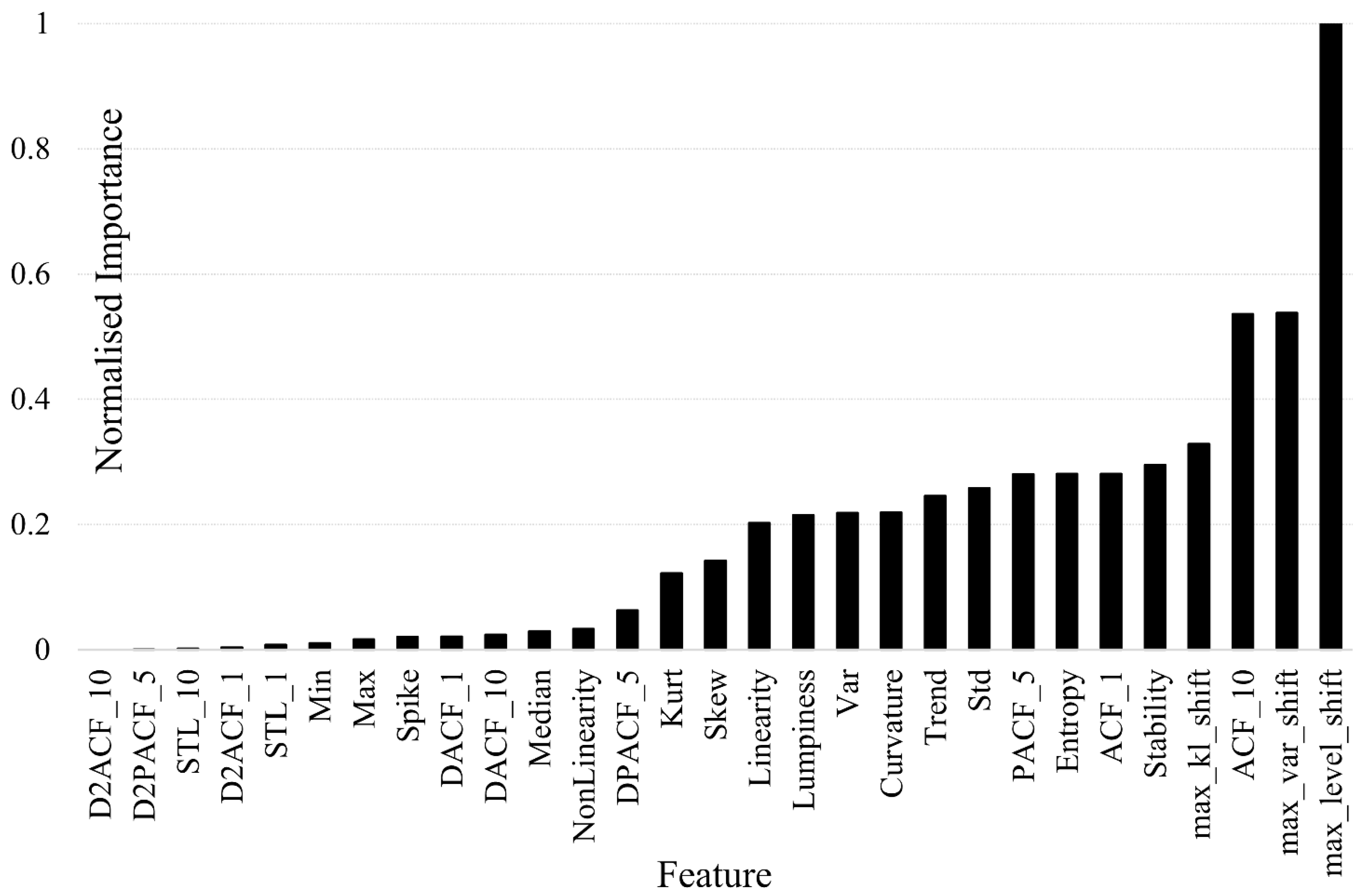
• Twenty-nine customized features are computed to distinguish the temporal properties of the five deformation trends, including autocorrelation, decomposition, and TS-based statistical metrics. Moreover, more effective features are introduced using a feature importance method based on the RF model.
• We assess the performance of algorithms based on False Alarm Rate (FAR) values in 99% confidence intervals to assess the impact of misclassifications in big DInSAR data analysis.
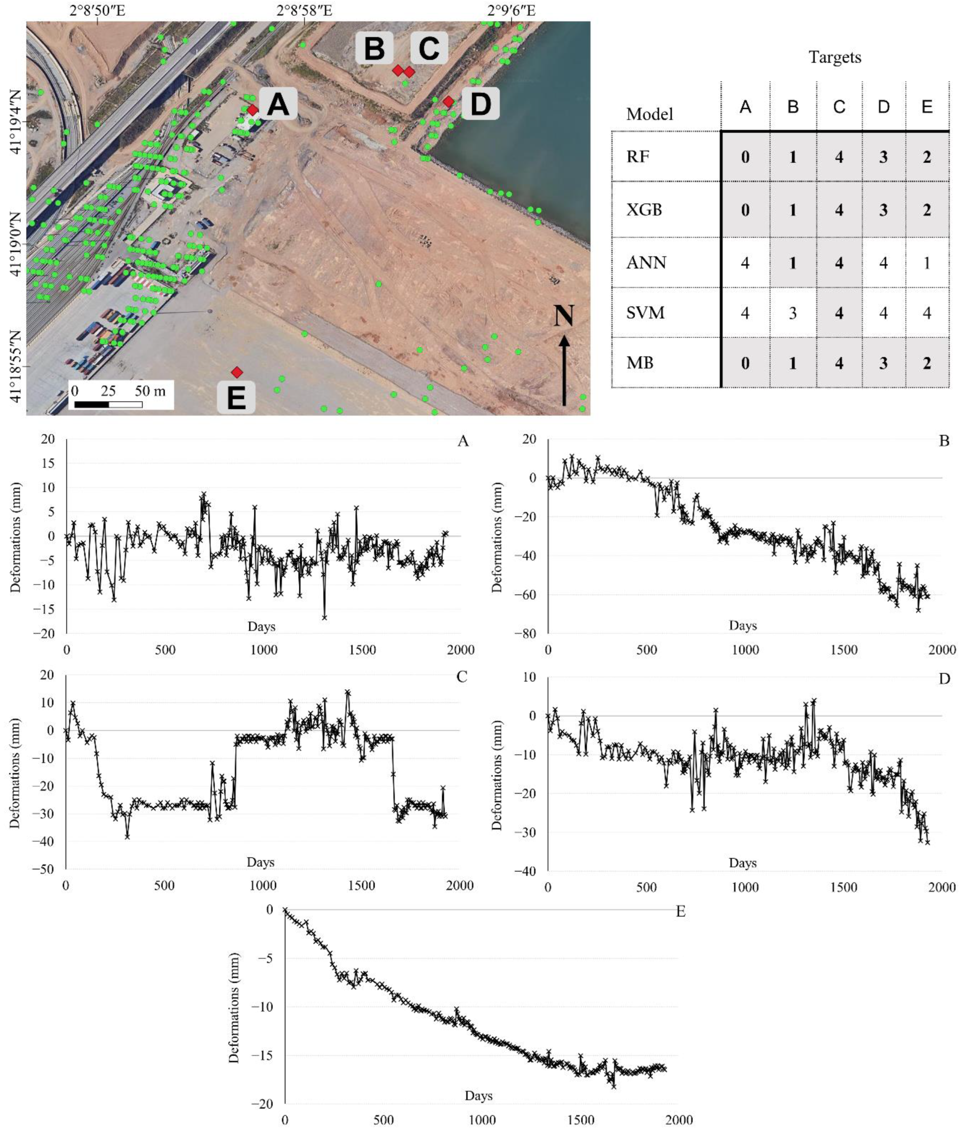
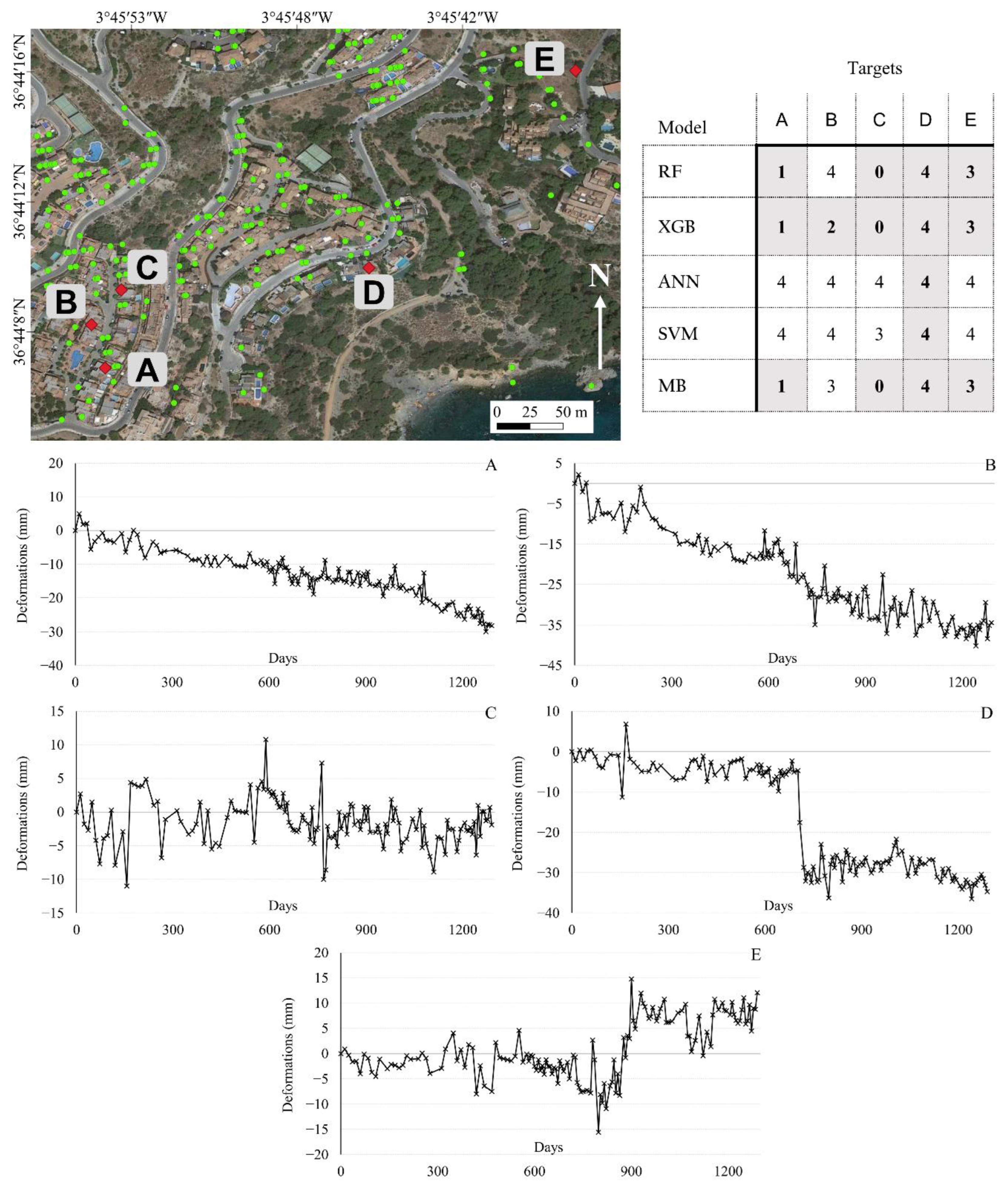
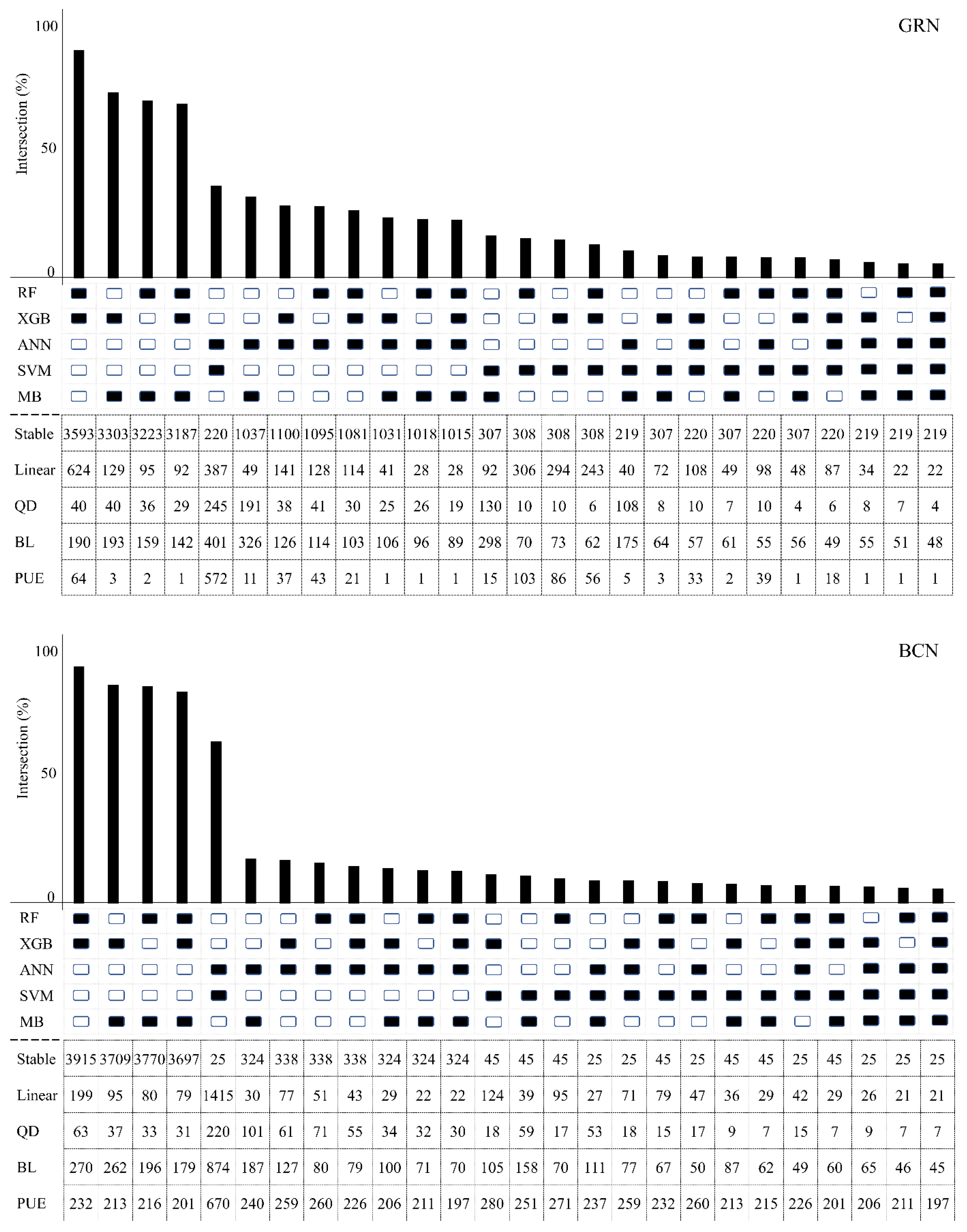
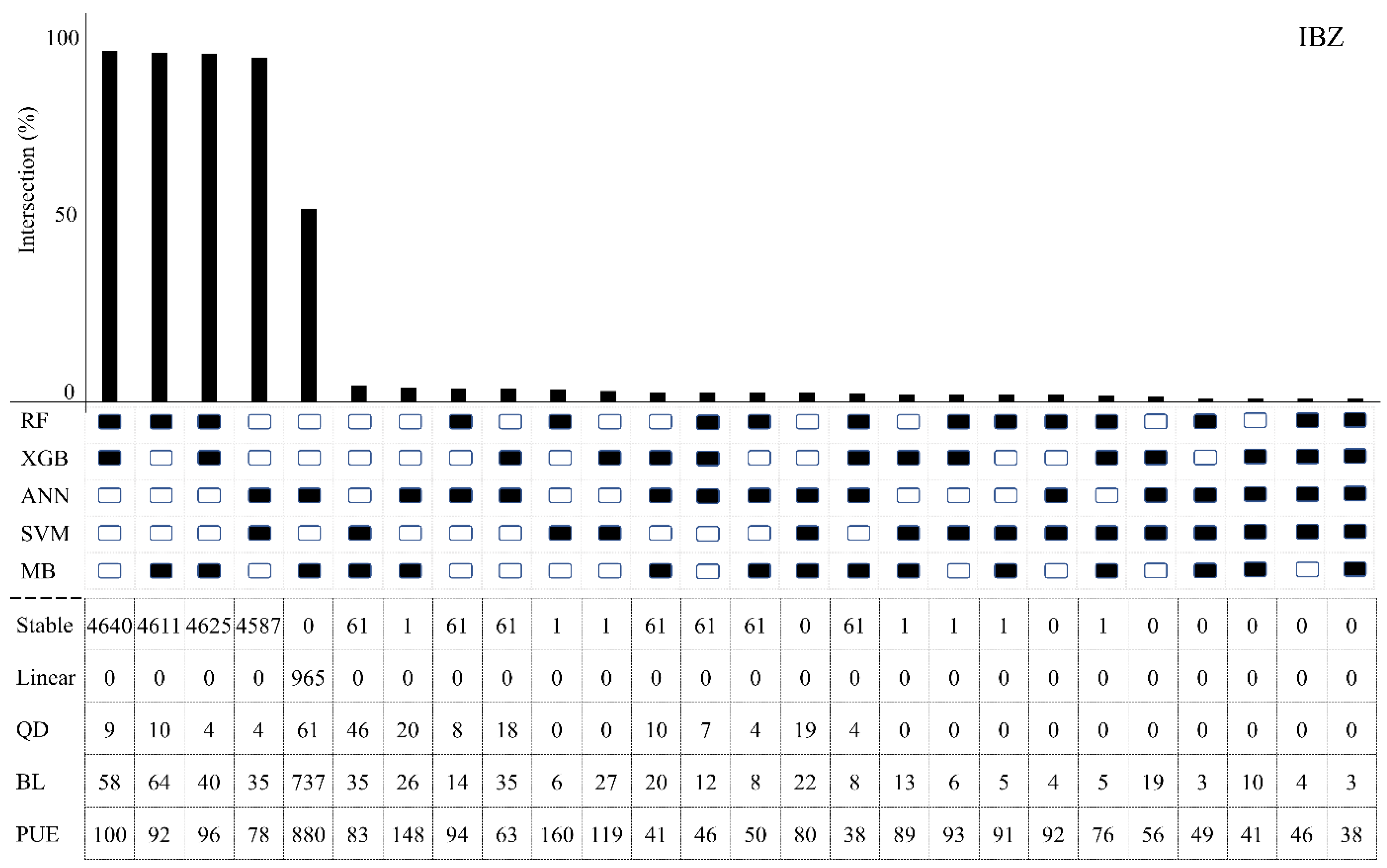
• Two validation steps are evaluated to examine the reliability of the proposed models, consisting of two deformation case studies in Spain and analysing the intersection of the proposed models and a benchmark classifier (the Model-Based (MB) method) classification results.

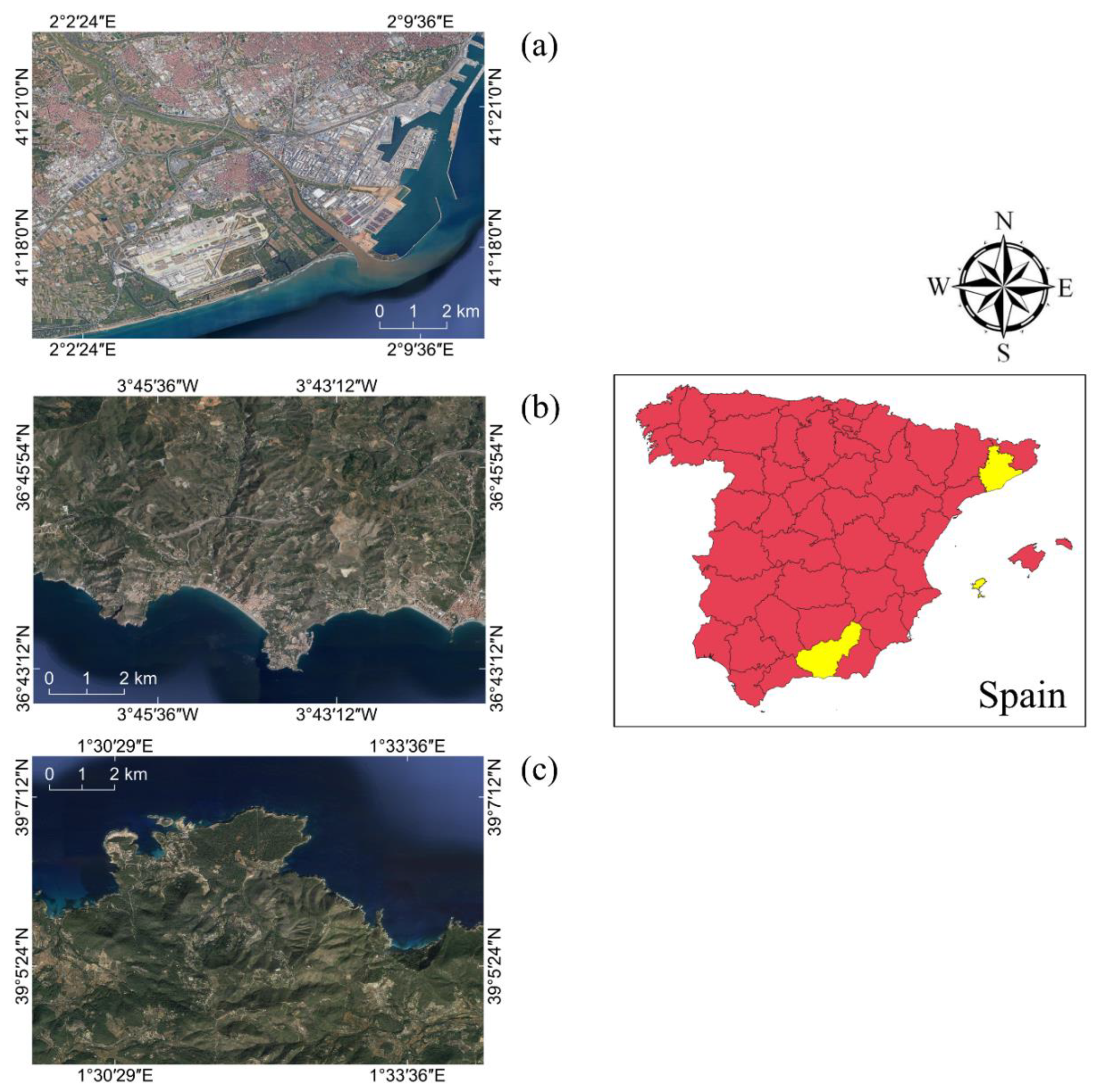
This article is structured as follows. Section 2 presents three datasets utilized in this study, along with characteristics and visual examples of each class. Afterward, the classification algorithms and definitions of TS-based features are explained in Section 3. Accuracy and validation assessment metrics are also presented in this section. Section 4 first assesses the performance of classification algorithms, and then the importance of customized features and validation of proposed methods are discussed. Finally, limitations and suggestions are discussed in Section 5, and some concluding remarks are provided in Section 6.

2. Dataset

2.1. Deformation Time Series

In this study, TSs from three different datasets (

Table 1. Characteristics of the three SAR datasets, along with the duration and average interval of interferograms.

Dataset	Satellite	#Observations in TS	Acquisition Span	Duration (Days)	Average Interval (Days)
GRN	Sentinel-1	138	10 March 2015–26 September 2018	1296	9.4
BCN	Sentinel-1	249	06 March 2015–19 June 2020	1926	7.7
IBZ	Sentinel-1	171	01 January 2017–27 February 2020	1152	6.7

) were used, which were generated using the PSI chain of the Geomatics Division of CTTC (PSIG) [40]. The Granada (GRN, Figure 1b) dataset was applied to train and test the proposed models, whereas the two other datasets were used for accuracy assessment and validation purposes. The TSs of GRN, Barcelona (BCN, Figure 1a), and Ibiza (IBZ, Figure 1c) were extracted from 138, 249, and 171 Sentinel-1 A/B images, respectively.

2.2. Reference Samples

DInSAR outputs include two main displacement categories: moving and nonmoving points. The TSs are first categorised into two primary classes, i.e., stable and unstable; then, the unstable TSs are categorised into predefined classes. The four most common unstable TS classes, along with the stable TS class, are introduced (see more details in [4,5]):

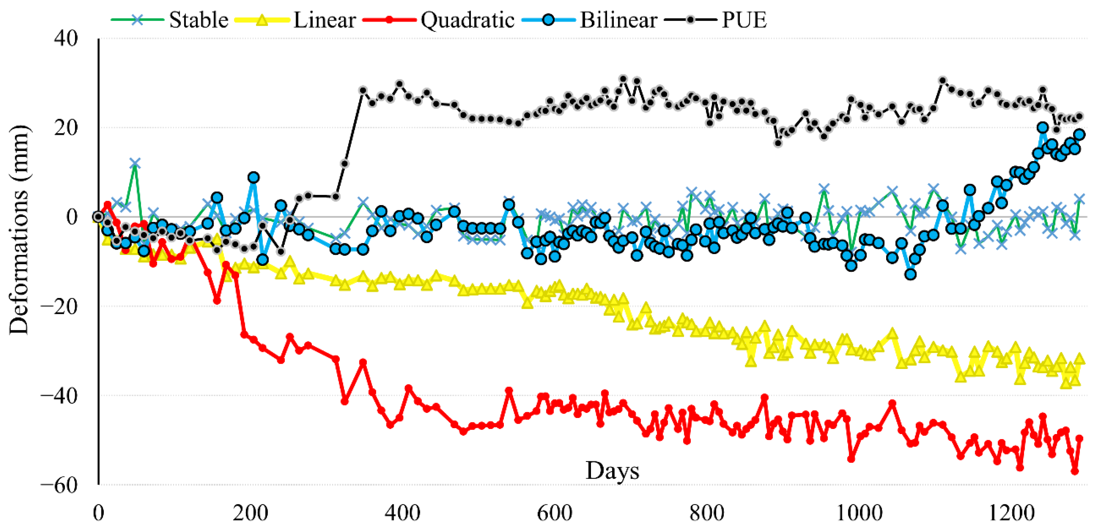
• Stable: The Stable class includes the nonmoving targets (see the green trend in Figure 2), i.e., the TS is dominantly characterized by random fluctuations included approximately between −5 and +5 mm. This class contains points for which significant deformation phenomena have not been detected during the observation period.
• Linear: A constant velocity (i.e., a slope) characterizes the TS, meaning that the deformation constantly increases or decreases over time (yellow trend in Figure 2).
• Quadratic: The deformation TS can be approximated by a second-order polynomial function, which demonstrates displacements characterized by continuous movements (red trend in Figure 2).
• Bilinear: The second nonlinear class includes two linear subperiods separated by a breakpoint (blue trend in Figure 2). This class mainly reflects an increasing deformation rate after a breakpoint, as in the case of collapse of a landslide or an infrastructure failure.
• PUE: Despite two steps of PUE removal in the PSIG procedure, there may still be TS affected by deformation jumps (see the black trend in Figure 2). Considering the C-band wavelength of Sentinel-1, the PUE value is about 28 mm (i.e., half the wavelength). Since the PUE value may change depending on the noise source [5], those TSs affected by vertical jumps of −15 to 28 mm (and greater than 28 mm) are classified as PUE. Indeed, the TS is divided into two or more segments by jumps, where separated segments are characterized by stable behaviour with different observation values (i.e., y-intercept). For example, the segment before the jump in the black trend of Figure 2 has values of approximately zero, while it is close to 30 mm in the second segment.

It should be noted that these classes are defined based on dominant trends inside the TS. For instance, the Stable TS of Figure 2 contains several points with values out of the [−5, +5] mm interval; however, these single points are not characterizing a representative trend. Moreover, Stable, Linear, and Quadratic trends can contain periodic fluctuations, while the TS is still following the dominant trend.

In this study, 1000 samples per class were classified by DInSAR experts from the GRN dataset. They were used first to train the proposed models and then evaluate the obtained accuracies. Seventy percent of the samples were used for training and the remaining 30% for testing.

3. Method

Six ML/DL algorithms and one model-based method were selected to evaluate the aforementioned datasets. In this section, first, an overview of each model is provided; then, in Section 3.2, we illustrate the metrics that are employed as features with the aim of improving the performance of the adopted models. Finally, Section 3.3 presents the accuracy assessment and the validation procedure.

3.1. Models

3.1.1. Support Vector Machine (SVM)

The SVM model is a kernel-based learning algorithm with a linear binary form to assign a boundary between two classes. In the case of multiclass supervised learning, SVM uses training samples to determine nonlinear hyperplanes (or margins), separating the classes optimally. The concept of support vectors refers to estimating the maximum separating margins. The SVM model has been effectively used in TS and sequence classifications [41]. Defining the kernel function is the most challenging part of SVM. The kernel selection and its parameters highly affect the performance of SVM. In this study, a radial basis function was chosen as the kernel, which has been widely utilized [42]. The kernel parameter, gamma, was evaluated using a diagnostic tool (i.e., a validation curve) to tune the model from the underfitting and overfitting performances.

Additionally, a developed version of SVM, based on the Dynamic Time Warping (DTW) distance, is implemented in [43]. Inspired by the works [44,45,46], an SVM-DTW employing a Global Alignment Kernel (GAK) was applied in our implementation.

3.1.2. Random Forest (RF)

Two learning methods have been extensively proposed in ML studies, bagging and boosting, which combine several learners to form a learner with better performance [47]. The bagging learners, such as RF, are independently built and trained parallelly. In fact, RF is one of the most popular ensemble ML models based on a simple nonparametric classification algorithm, the DT [48]. RF makes use of multiple DTs by incorporating a mean estimator to increase the accuracy by bagging learning [48]. RF is less sensitive to overfitting due to assembling various structures of trees and splitting points. It can also handle missing data and be robust to outliers and noise. Since the most influential parameter is the number of trees, a validation curve is generated to identify its optimum value. RF is also employed to evaluate the importance of the proposed features adopted in the classification. This subject is discussed in Section 4.2.

3.1.3. Extreme Gradient Boosting (XGB)

Boosting learners are sequential ensemble methods, where models are built considering previous performance. Gradient boosting models are based on an optimisation problem to minimize the differentiable loss function of the model by adding weak learners using gradient descent. The XGB model is designed by DT to improve the processing time and performance of predictions. Encountering missing values, flexibility, and parallel processing are the most notable features of XGB [47].

3.1.4. Artificial Neural Network (ANN)

ANN is a feedforward DL network and a Neural Network (NN) supervised algorithm learning via backpropagation training [49]. It comprises three types of layers, including input, output, and hidden layers. Multiple perceptron layers, i.e., the hidden layers, can learn a nonlinear function for classification purposes. The supervised ANN trains a large portion of input–output sets to investigate a model with the highest correlation among inputs and outputs. Numerous weights and biases are adjusted throughout the training stage to minimize the error of the layer above. The backpropagation algorithm computes the partial derivatives of the error function considering the biases and weights in the backward pass [50]. In this study, 200 iterations of three hidden layers are examined to drive the optimum structure of ANN.

3.1.5. K-Nearest Neighbour (KNN)

KNN is one of the most common ML methods, assuming similar characteristics exist among samples. Considering its properties in representation, prediction, and implementation, KNN has been widely applied in various classification and regression applications. KNN is structured on a detecting similarity by a majority vote among the identical nearest neighbours of each training sample. KNN can also consider a predefined radius to compute similarities [51]. Despite its simplicity, KNN is categorized as a lazy learner algorithm since input samples are stored to train during the classification. This algorithm is also inefficient in computational procedures, as it computes numerous distances among training samples.

3.1.6. Model-Based (MB)

The MB approach [5] distinguishes the dominant trend of each TS and was proposed as an advanced version of the PS Time Series method [4] that clusters the TS deformation into seven predefined trends. This model implements multiple statistical tests to categorise TSs by maximising the similarity with the predefined displacement types. The MB method analyses each TS based on three main characteristics, i.e., nonmoving, linear, and nonlinear behaviours. It was stated that this model could classify synthetic and real TSs with around 77% accuracy [5], where the highest accuracies were reported for PUE and Stable trends. We implemented this model to evaluate the performance of the proposed ML/DL models.

3.2. Time Series Features

Generally, a TS includes a list of deformation values associated with the correspondent acquisition times. A TS can be defined by fundamental patterns, such as temporal trend, seasonality, and cycles. The trend is the dominant or long-term behaviour of a TS, such as linear or a prevalent increasing or decreasing change, which is usually combined with the cycle as a trend-cycle component [52]. Seasonal pattern refers to regular fluctuations with a fixed frequency (e.g., daily, weekly, monthly, etc.). It is worth mentioning that the following features are available in the tsfeatures Python library and R CRAN package.

3.2.1. General Features

Considering the characteristics mentioned above, a set of features have been employed to summarize the TS properties in this work (see

Table 2. List of 29 computed features.

Category	#Features	Features
General	7	var, std, median, min, max, skewness, kurtosis
Autocorrelation Function (ACF)	6	ACF_1, ACF_10, DACF_1, DACF_10, D2ACF_1, D2ACF_10
Partial Autocorrelation Function (PACF)	3	PACF_5, DPACF_5, D2PACF_5
Seasonal and Trend Decomposition Using LOESS (STL)	6	trend, spike, linearity, curvature, STL_1, STL_10
Other	7	nonlinearity, entropy, lumpiness, stability, max_level_shift, max_var_shift, max_kl_shift

). This step is aimed at reducing the size of the input data and simplifying the information carried out by the input itself. First, five general statistics, variance (Var), standard deviation (Std), median, minimum (min), and maximum (max) values, are computed to inform an initial vision of the structure of the dataset. Additionally, two coefficients related to the statistical distribution in the data for each TS are calculated: skewness and kurtosis, which are both measures of the deviation from the normal distribution. In the DInSAR TS products, the outliers may refer to various sources of errors.

3.2.2. Autocorrelation Function (ACF) and Partial Autocorrelation Function (PACF) Features

In addition to seven general features, 27 estimators are taken into account to analyse the correlation among the values in each TS. The Autocorrelation Function (ACF) measures the correlation between the values in a TS. The values of the autocorrelation coefficients are calculated as follows:

$$r_k=\frac{{{\displaystyle \sum }}_{t=k+1}^T\left(y_t-\overline{y}\right)\left(y_{t-k}-\overline{y}\right)}{{{\displaystyle \sum }}_{t=1}^T{\left(y_t-\overline{y}\right)}^2}$$

(1)

where T indicates the length of the TS, and $y_t$ and $\overline{y}$ refer to the deformation value at epoch t and its average, respectively. Generally, autocorrelation is computed to identify nonrandomness in the data. To simplify computation time regarding ACF-related parameters, six features are computed to summarize the degree of autocorrelation within a TS (see Table 2). ACF_1 is the first calculated autocorrelation coefficient. ACF_10 is the sum of squares of the first ten autocorrelation coefficients. Moreover, autocorrelations of the changes provide a TS without temporal changes (e.g., trend and seasonality). Thus, differentiating is first calculated to compute the differences between consecutive observations within a TS, and then the ACF parameters are computed. DACF_1 obtains the first autocorrelation coefficient from the differenced data. DACF_10 measures the sum of squares of the first ten autocorrelation coefficients from the differenced series. The first derivative of TSs derives velocity of deformation. Additionally, D2ACF_1 and D2ACF_10 provide similar values corresponding to the twice-differenced series (i.e., the second-order differencing operation from the consecutive differences). In fact, the second derivative obtains the displacement acceleration in TSs. Similarly, three features (see Table 2) are computed by the Partial Autocorrelation Function (PACF) of the first five partial autocorrelation coefficients, including PACF_5, DPACF_5, and D2PACF_5. The partial autocorrelation assesses the relationship of observations with shorter lags. Consequently, ACF and PACF provide an overview of a TS’s nature and temporal dynamics [52,53].

3.2.3. Seasonal and Trend Decomposition Using the LOESS (STL) Features

The Seasonal and Trend decomposition using the LOESS (STL) method decomposes a TS into a trend ($T$) (i.e., trend-cycle), seasonal ($S$), and remainder (containing components apart from the three mentioned ones, $(R$) components [54]:

$$y_t=T+S+R$$

(2)

Six features (see Table 2) are extracted by STL decomposition to investigate the trend-cycle and remainder components: (1) Trend: it shows the strength of a cyclic trend inside a TS from 0 to 1 (see Equation (3)). (2) Spike: it represents the prevalence of spikiness in the remainder component of the STL decomposition. (3) Linearity and (4) Curvature features estimate the linearity and curvature of the trend component by applied linear and orthogonal regressions, respectively [54,55]. (5) STL_1 and (6) STL_10 represent the first autocorrelation coefficient and the sum of squares of the first ten autocorrelation coefficients of the remainder series, respectively.

$$Trend=\max (0,1-\frac{Var\left(R\right)}{Var\left(T+R\right)})$$

(3)

3.2.4. Other Features

Another set of features is extracted to develop further analysis on deformation TS, including nonlinearity, entropy, lumpiness, stability, max_level_shift, max_var_shift, and max_kl_shift (see Table 2). Nonlinearity determines the log of a ratio consisting of the sum of squared residuals from a nonlinear ($SS{E}_1$) and linear ($SS{E}_0$) autoregression by Teräsvirta’s nonlinearity test (Equation (4)), respectively, [56].

$$X^2=T\log \frac{SS{E}_1}{SS{E}_0}$$

(4)

The entropy metric measures the spectral density of a TS, quantifying the complexity or the amount of regularity. Lumpiness and stability features measure the variance of the means and the variances on nonoverlapping windows, which provide information on how a TS is free of trends, outliers, and shifts. Finally, the last three features, max_level_shift, max_var_shift, and max_kl_shift, denote the largest shifts in mean, variance, and Kullback–Leibler divergence (a measure between two probability distributions) of a TS based on overlapping windows, respectively. These features may distinguish valuable structures regarding the TS with jumps.

3.3. Accuracy and Validation Assessments

A way to assess the performance of a multiclass classification process is a confusion matrix or contingency table. Several metrics can be extracted through a confusion matrix, whereas four of them are employed in this study, including Overall Accuracy (OA), precision, F₁-score, and False Alarm Rate (FAR). OA obtains the classification performance by proportioning correctly classified samples to the total number of samples. Precision indicates the prediction performance in each class by the ratio of correctly classified samples to the total number of predicted samples of the correspondent class. Additionally, F₁-score computes a balanced average of precision and recall (i.e., the number of correctly classified samples to the total of a class). FAR, also referred to as false positive rate, represents the portion of the incorrectly classified samples to the total of a class, reflecting that a model may identify a target as a moving deformation without significant movement. Based on the limited number of testing samples, the Confidence Interval (CI) was computed considering a 99% significance level of the normal distribution (approximately equal to 2.58): $FAR\pm CI$ (Equation (5))

$$CI=2.58\times \sqrt{\frac{FAR\times \left(1-FAR\right)}{N}}$$

(5)

where N is the total number of other classes.

The accuracy assessment can only evaluate the prelabelled samples (i.e., seen data). Thus, two validation stages are proposed to provide an unbiased evaluation of the trained models for those data that have not been previously labelled (i.e., seen data). First, the TSs of two case studies are predicted using the proposed models and the MB approach [5], in order to investigate the performance of the models. Afterward, an intersection visualisation process, UpSet [57], is utilized to compute pairwise intersections of the classification results of five models (SVM, RF, XGB, ANN, and MB). The visualisation consists of the percent of intersection among all pairs of five selected models and the number of TSs classified as similar classes. The five models have first classified five thousand random samples per three data collections, then the portion of intersections and number of similar TSs in each class have been computed. This outcome enables a visual understanding of the performance of classification models and the quantitative analysis of the predictions. Since a large portion of the TSs have no significant movements (i.e., they belong to the Stable class), the similarities in the number of Stable points can present valuable information on the reliability of the models.

4. Results and Discussion

Six ML models were ensembled to classify deformation TS into five classes. The reference samples were divided into training and testing sets, with a 70–30% split ratio. The classification algorithms were set by configuration parameters in

Table 3. Configuration parameters for classification algorithms.

Algorithm	Parameters	Description
SVM	c = 1	regularisation parameter
	kernel = rbf	Radial Basis Function (RBF) maps input data
	gamma = auto	kernel coefficient
SVM-DTW	c = 1	regularisation parameter
	kernel = gak	Radial Basis Function (RBF) maps the input data
	gamma = auto	GAK function for mapping input data
RF	n_estimators = 150	number of trees
	criterion = gini	a function to measure the quality of a split
	max_depth = none	maximum depth of trees
	random_state = 10	controls the randomness of input samples
XGB	learning_rate = 0.3 booster = gbtree	shrinks the contribution of trees tree-based model to run at each iteration
ANN	hidden_layer_sizes = 3	number of hidden layers apart from input and output layers
	hidden_layer_neurons= [0,100]	number of neurons in each hidden layer
	activation = relu	the rectified linear unit function, returns f(x) = max (0, x)
	solver = adam	the solver for weight optimisation
	learning_rate = 0.001	controls the step-size in updating the weights
	alpha = 0.0001	regularisation term
KNN	n_neighbours = 5	number of neighbours for queries.
	weights = distance	weight points by the inverse of their distance
	metric = minkowski	the distance metric to use for the tree

. Moreover, the implementation was performed in Python using the sklearn, tslearn, and xgboost libraries. The method was carried out using an Intel Core i7 machine with 32 GB of RAM and an Intel UHD Graphics 630 GPU card.

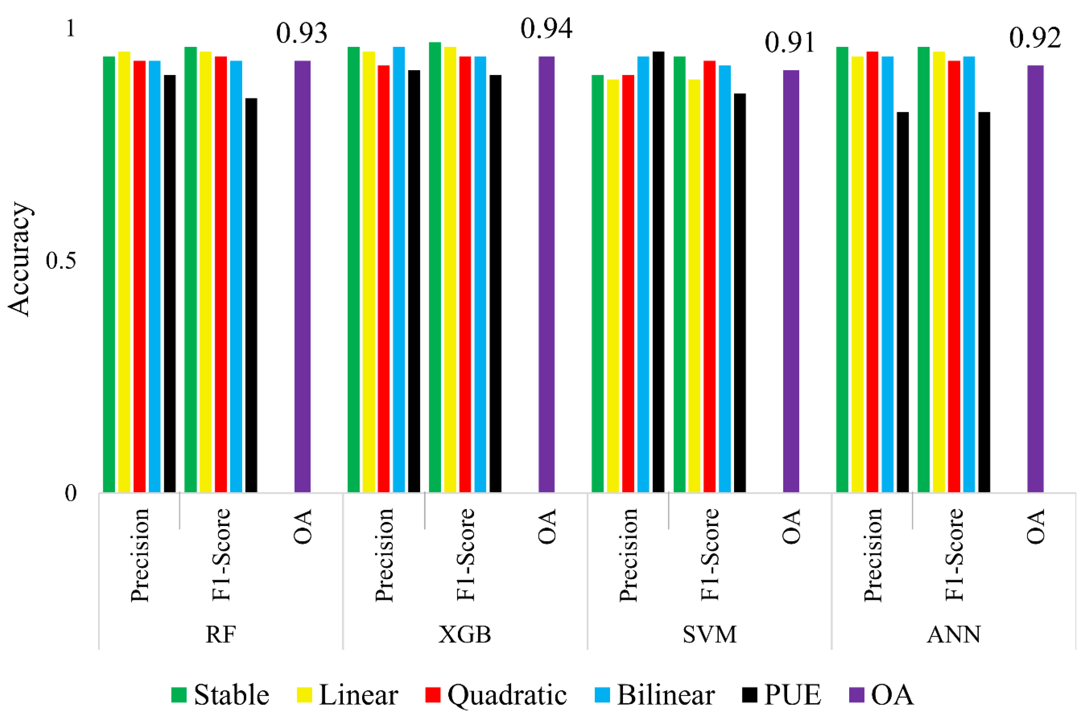
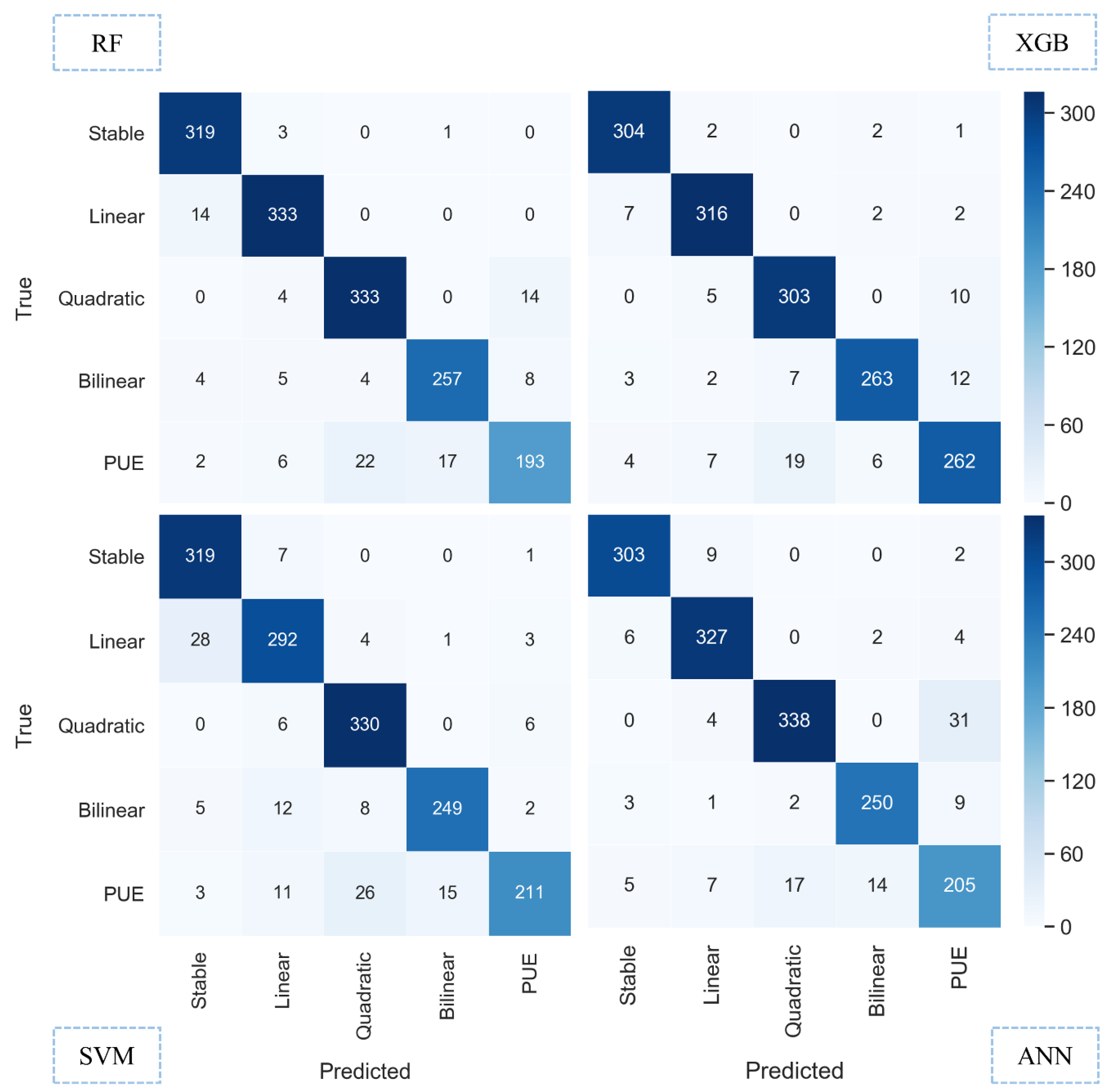
4.1. Classification Performance

Table 4. Accuracy and computational time (samples/second) performance without considering customized features.

	Model
	SVM	SVM-DTW	RF	XGB	ANN	KNN
OA	0.82	0.83	0.84	0.83	0.9	0.78
Computational Speed	190	37	296	288	218	152

presents the performance of six ML/DL models using 5000 deformation TSs with the average OAs. The highest and lowest accuracies were achieved by the ANN and KNN models, respectively. The OAs of other models ranged from 0.82 to 0.84. It was expected that the KNN model would be barely an appropriate classifier to categorise multiple TS, although SVM-DWT shows higher OA than SVM as an expense of its highest computation time. Since KNN and SVM-DTW were not efficient in terms of accuracy and computational process, in the following sections only four models are discussed: SVM, RF, XGB, and ANN.

In terms of computational time of the proposed models, we excluded the preprocessing steps (e.g., data preparation, data normalisation, train/test splitting, etc.,) from the speed of the models (approximately one minute). It was due to the fact that these steps were performed before training and prediction steps. As stated in Table 4, SVM-DTW and RF were the slowest and fastest models in classifying deformation TSs. There was also an insignificant difference between RF and XGB computational times.

Figure 3 shows the precision and F₁-score values of all classes per model, considering the customized features. The addition of the proposed features significantly increased the accuracy performance, exceeding 0.11 for XGB and 0.09 for RF and SVM. The ANN model improved by 0.02. Regarding the precision, all models were able to identify the five classes with an accuracy higher than 0.9, except the PUE class by ANN and Linear class by SVM. In total, the Stable and PUE classes were the most and least accurate classes, respectively. These outcomes indicate a strong performance of ML- and DL-based algorithms in classifying deformation TSs after employing appropriate features. The same can be concluded from the F₁-score values, demonstrating accuracy higher than 0.9 for almost all classes in the proposed models.

Figure 4 shows confusion matrices for the four models, where the values represent the predicted samples per class. The values along the diagonals indicate the number of correctly classified samples. Additionally, other cells show the number of confused (misclassified) samples. It can be concluded that PUE and Quadratic samples were confused more than the other cases, along with several samples to Bilinear. Since PUE, Quadratic, and Bilinear classes are characterized by nonlinear trends, it can be stated that most of the misclassifications occur for nonlinear trends. Among the proposed models, RF and XGB were less affected by singularities of nonlinear trends. However, around 5% of the Linear TSs were incorrectly identified as Stable by RF. Approximately 9% of similar misclassification was also found in SVM. This can be due to a similarity in Stable- and Linear-trend behaviour, where Linear trends with small values of the slope can be confused as Stable. In total, the most confusing samples occurred in the PUE class, ranging from 12% to 20%, approximately.

Table 5. FAR values (%) of the four proposed models, integrated by the CIs of a 0.01 level of significance.

	Model
Class	RF	XGB	SVM	ANN
Stable	$1.67\pm 0.96$	$1.15\pm 0.79$	$3.06\pm 1.30$	$1.16\pm 0.79$
Linear	$1.53\pm 0.93$	$1.34\pm 0.86$	$3.06\pm 1.30$	$1.78\pm 0.99$
Quadratic	$2.24\pm 1.12$	$2.18\pm 1.09$	$3.28\pm 1.35$	$1.66\pm 0.97$
Bilinear	$1.45\pm 0.87$	$0.81\pm 0.65$	$1.28\pm 0.82$	$1.27\pm 0.82$
PUE	$1.72\pm 0.94$	$2.06\pm 1.05$	$0.95\pm 0.71$	$3.69\pm 1.38$

indicates another relevant aspect of classification analysis, which has not been appropriately considered: the FAR. As previously stated, the FAR quantifies the probability of erroneously assigning a stable TS to an unstable class.

Except in the SVM model, almost all trends presented FAR values smaller than 3%. Although boosted learning is one of the best ways to decrease the FAR, the XGB model did not reach better estimation than other models. Moreover, the DInSAR TS data collection is highly affected by various sources of noise and outliers, which add distortions, preventing the proposed models from identifying the relevant trends with higher accuracy. For example, ANN identified the least number of incorrect samples, but the FAR of the PUE class varies from 2.31% to 5.07%, indicating the impact of noise on the estimation (i.e., PUE trend is defined based on noise, so-called a phase unwrapping noise). Furthermore, FAR amounts are critical in cases where nonmoving targets are incorrectly classified as moving targets, which wrongly alarms policymakers to carry out investigations and fieldwork over safe areas (i.e., economic disadvantages).

4.2. Feature Importance

As mentioned in Section 3.2, general and advanced features were integrated into the methodology to improve the classification performance. In this study, we employed an implicit feature selection of the RF, the Gini approach [48], to calculate the importance of added features, as shown in Figure 5. The most and least effective features were max_level_shift and D2ACF_10, respectively. Var and Std were the only features among the seven general statistics that improved the classification performance. The importance of shift-based features indicates their suitability in providing essential information on trends, particularly on nonlinear TS, as the values of nonlinear trends typically include large changes (i.e., shifts) affecting the mean and variance. Furthermore, ACF and PACF computations provide beneficial impacts on the classification, demonstrating the capability of these features on temporal dynamics detection. However, the first- and second-order differential of ACF and PACF did not lead to a significant performance improvement, except for DPACF_5. Similarly, the autocorrelation STL decomposition components slightly influenced the classification performance. On the other hand, three other STL features (e.g., Trend, Linearity, and Curvature) obtained importance values higher than 0.2. Consequently, the outcomes of the TS-based feature importance analysis (Figure 3 and Figure 4) demonstrate the impact of integrating features, which estimates the temporal properties of deformation TSs. Classification by representative features can help hasten the training process, reducing computational time while improving the generalisation of a specific model and its ability to perform accurately within new unseen datasets.

4.3. Validation of Proposed Algorithms

We present two validation stages to investigate the performance of the proposed methods for predicting the class of unseen data. Firstly, two case studies were analysed. Figure 6 and Figure 7 show several moving and nonmoving points in Barcelona Harbour and over a landslide in the Granada region. These figures also include the TSs of the targets and the corresponding classes.

Figure 6 shows the five selected targets and TSs in Barcelona Harbour, along with a table indicating the predicted classes by the five models. The numbers in the table refer to classes (e.g., Stable, Linear, Quadratic, Bilinear, and PUE). Considering the TS of each target, A is Stable, B is Linear, C is PUE, D is Bilinear, and E is Quadratic. The results demonstrate that ANN and SVM incorrectly predicted targets A, D, and E. However, all models could accurately identify the PUE point. It should also be noted that RF, XGB, and MB could recognize all these selected samples.

Figure 7 shows a region affected by a landslide in the Granada region, close to an urban area [58,59]. In this region, the TSs are characterized by Linear (A), Quadratic (B), Stable (C), PUE (D), and Bilinear (E) trends. Among the proposed models, XGB could classify all points correctly. However, all models predicted the target D correctly as PUE. Similarly, to the Barcelona Harbour case study, ANN and SVM hardly distinguished the trends. However, RF and XGB could accurately detect the trends, as could MB. In conclusion, these case studies illustrate the performance of the trained models in identifying targets, which were not labelled previously.

In the second stage, a recent methodology, UpSet, was applied to the classification results of the proposed models to investigate the correlation among multiple pairwise intersections of the outcomes. Figure 8 provides three subfigures, showing the predicted 15,000 random samples in five classes and the intersection percent of identical TSs in each model. Analysis of intersections can drive two main conclusions.

First, the number of Stable targets in each intersection can be considered as an indicator of the classification performance. In fact, as the vast majority of PSs in the area of interest is not affected by any relevant displacement, the large number of Stable points in the intersection between two or more models is an indicator of classification robustness. We observe a significant correlation among RF, XGB, and MB results in the number of Stable samples, along with the portion of the intersection. On the other hand, a limited performance was observed by SVM and ANN, indicating weak identification performance.

Second, there are similarities among RF and XGB models to MB in the three datasets, indicating their reliability. However, these are not as much as in the GRN dataset compared to two other datasets. The most probable reason can be the lower number of values in the TS samples of this dataset. According to Table 1 (see Section 2.2), the average acquisition interval of GRN TS data is more extensive than other datasets, which causes a mediocre misclassification. Consequently, the primary purpose of this validation stage was to obtain similarities among the models. It also showed that the usual accuracy assessment may not be the most reliable criterion to decide on the performance of the classifiers. Additionally, the number of samples in a TS can affect the reliability of classification, considering the outcomes of GRN data.

4.4. Comparison of Machine Learning Algorithms with the Model-Based Method

The 5000 reference samples were classified using the MB method to analyse its accuracy and compare its performance with the proposed ML/DL algorithms. The ratio of correctly classified to total samples was approximately 83%. In Section 4.3, the performance of the ML/DL and MB models was also evaluated in identifying unlabelled samples and deformation phenomena. However, the comparison of proposed models with the MB method is not a straightforward evaluation. The MB is a multilevel method (it can be categorised as semisupervised learning), which detects predefined trends using certain assumptions that might bound its classification accuracy. Indeed, the categorised TSs satisfied various tests based on statistical definitions of the predefined trends. Therefore, the comparison is limited to computational efficiency, big data management, and parameter tuning.

Computational efficiency refers to a tradeoff between the speed of computations and performance accuracy. MB categorises samples faster than ML/DL models considering the time of computations. However, the performance of the proposed models is approximately 10% more accurate in the number of correctly classified TSs. Big datasets can also be managed by ML/DL algorithms more conveniently than MB. Additionally, the MB method is required for selection of an empirical threshold (i.e., parameter tuning) to identify accurately the trends inside TSs. However, this procedure is not similarly time-consuming and complex in ML/DL algorithms due to their generalisation potential. In conclusion, two critical points that can affect the comparison should be noted. First, model-based methods are generally faster than ML/DL even though they lack flexibility. In comparison, ML/DL strategies are considered as black-box solutions, lacking explainability. Furthermore, the accuracy assessment of these techniques cannot be completely identical. The accuracy of ML-based proposed models was reported by confusion matrices containing several performance indicators. However, the MB method’s performance is limited to the number of correctly classified samples, i.e., accuracy. Thus, it can be stated that ML/DL models can be more practical considering their advantages in accuracy and big data management.

5. Limitations and Future Works

The classification of deformation TSs was studied in this work using ML/DL algorithms integrated with customized features. The classification performance assessment showed an accurate identification of five dominant displacements trends. Furthermore, the FAR analysis and intersection-based validation presented more aspects regarding supervised learning in deformation detection. Consequently, several limitations and recommendations for future studies follow:

• Only a 1% misclassification may negatively affect the interpretation and decision-making based on the classification outcomes. For this reason, it is recommended to decrease these false alarms using a larger source of reference samples, which enables a more robust classification. Data refinement is also suggested to clean the TSs in terms of noise and errors.
• An unsupervised learning approach is recommended to (1) supply more reference samples for the subsequent supervised classification. This enables the improvement of deformation detection for supervised classifiers by decreasing misclassification. (2) This approach is also recommended for exploring further classes. DInSAR experts proposed the five trends of this study based on their experience. Thus, unsupervised learning will be considered to obtain further information on deformation TS classes.
• Despite the proposed five classes, the adopted algorithms can be used to classify particular cases of TS. Although the prevalent trends (including uncorrelated, linear, and nonlinear) were used in this research, a different trend can be detected by the proposed models. For instance, TS with specific anomalies may provide interesting case studies that illustrate significant movements in the final sections of TSs, enabling a continuous monitoring framework with fast update times to detect changes in the analysed TSs.
• Further improvements may be achieved by utilizing more advanced algorithms, such as CNN and Recurrent Neural Network (RNN). Although the neural networks have longer computational times and greater complexity, more accurate results may be derived for small-scale regions. On the other hand, the RF and XGB algorithms are proposed for deformation identification over wide areas due to the efficient performance in terms of computational time, complexity, and reasonable accuracy.

6. Conclusions

This study evaluated supervised ML/DL algorithms to classify ground motions in five classes using DInSAR TS and customized features. The customized features enhanced the classification performance. These features also summarized TSs using the limited number of values and improving the efficiency of ML models for big DInSAR data classification. Our study showed that ML algorithms could identify ground deformation with accuracies greater than 90%. Moreover, the results demonstrated that the customized features improved the performance by 10%. Two validation stages also highlighted the reliability of RF and XGB models in predicting classes for unlabelled data. An MB method was also applied to compare classification similarities in these stages. We addressed what advantages ML algorithms can offer to ground deformation classification, such as accuracy and large DInSAR data management. It is worth noting that several unsatisfactory performances were pointed out regarding the FARs and classification of short TSs. Owing to the critical importance of moving-target FAR values in ground deformation detection, more advanced research is required to decrease FARs. Finally, our work indicated the applicability of ML algorithms in DInSAR TS analysis and prepared a framework for ML future investigations of ground deformation classification.

References

1. Crosetto, M.; Solari, L.; Mróz, M.; Balasis-Levinsen, J.; Casagli, N.; Frei, M.; Oyen, A.; Moldestad, D.A.; Bateson, L.; Guerrieri, L.; et al. The Evolution of Wide-Area DInSAR: From Regional and National Services to the European Ground Motion Service. Remote Sens. 2020, 12, 2043. [Google Scholar] [CrossRef]
2. European Ground Motion Service. Available online: https://land.copernicus.eu/pan-european/european-ground-motion-service (accessed on 30 May 2022).
3. Cigna, F.; Del Ventisette, C.; Liguori, V.; Casagli, N. Advanced Radar-Interpretation of InSAR Time Series for Mapping and Characterization of Geological Processes. Nat. Hazards Earth Syst. Sci. 2011, 11, 865–881. [Google Scholar] [CrossRef]
4. Berti, M.; Corsini, A.; Franceschini, S.; Iannacone, J.P. Automated Classification of Persistent Scatterers Interferometry Time Series. Nat. Hazards Earth Syst. Sci. 2013, 13, 1945–1958. [Google Scholar] [CrossRef] [Green Version]
5. Mirmazloumi, S.M.; Wassie, Y.; Navarro, J.A.; Palamà, R.; Krishnakumar, V.; Barra, A.; Cuevas-González, M.; Crosetto, M.; Monserrat, O. Classification of Ground Deformation Using Sentinel-1 Persistent Scatterer Interferometry Time Series. GISci. Remote Sens. 2022, 59, 374–392. [Google Scholar] [CrossRef]
6. Intrieri, E.; Raspini, F.; Fumagalli, A.; Lu, P.; Del Conte, S.; Farina, P.; Allievi, J.; Ferretti, A.; Casagli, N. The Maoxian Landslide as Seen from Space: Detecting Precursors of Failure with Sentinel-1 Data. Landslides 2018, 15, 123–133. [Google Scholar] [CrossRef] [Green Version]
7. Raspini, F.; Bianchini, S.; Ciampalini, A.; Del Soldato, M.; Montalti, R.; Solari, L.; Tofani, V.; Casagli, N. Persistent Scatterers Continuous Streaming for Landslide Monitoring and Mapping: The Case of the Tuscany Region (Italy). Landslides 2019, 16, 2033–2044. [Google Scholar] [CrossRef] [Green Version]
8. Brengman, C.M.J.; Barnhart, W.D. Identification of Surface Deformation in InSAR Using Machine Learning. Geochem. Geophys. Geosystems 2021, 22, e2020GC009204. [Google Scholar] [CrossRef]
9. Zheng, X.; He, G.; Wang, S.; Wang, Y.; Wang, G.; Yang, Z.; Yu, J.; Wang, N. Comparison of Machine Learning Methods for Potential Active Landslide Hazards Identification with Multi-Source Data. ISPRS Int. J. Geo-Inf. 2021, 10, 253. [Google Scholar] [CrossRef]
10. Fadhillah, M.F.; Achmad, A.R.; Lee, C.W. Integration of Insar Time-Series Data and GIS to Assess Land Subsidence along Subway Lines in the Seoul Metropolitan Area, South Korea. Remote Sens. 2020, 12, 3505. [Google Scholar] [CrossRef]
11. Novellino, A.; Cesarano, M.; Cappelletti, P.; Di Martire, D.; Di Napoli, M.; Ramondini, M.; Sowter, A.; Calcaterra, D. Slow-Moving Landslide Risk Assessment Combining Machine Learning and InSAR Techniques. Catena 2021, 203, 105317. [Google Scholar] [CrossRef]
12. Nava, L.; Monserrat, O.; Catani, F. Improving Landslide Detection on SAR Data through Deep Learning. IEEE Geosci. Remote Sens. Lett. 2021, 19, 4020405. [Google Scholar] [CrossRef]
13. Lu, P.; Casagli, N.; Catani, F.; Tofani, V. Persistent Scatterers Interferometry Hotspot and Cluster Analysis (PSI-HCA) for Detection of Extremely Slow-Moving Landslides. Int. J. Remote Sens. 2012, 33, 466–489. [Google Scholar] [CrossRef]
14. Liu, Q.; Zhang, Y.; Wei, J.; Wu, H.; Deng, M. HLSTM: Heterogeneous Long Short-Term Memory Network for Large-Scale InSAR Ground Subsidence Prediction. IEEE J. Sel. Top. Appl. Earth Obs. Remote Sens. 2021, 14, 8679–8688. [Google Scholar] [CrossRef]
15. Fiorentini, N.; Maboudi, M.; Leandri, P.; Losa, M.; Gerke, M. Surface Motion Prediction and Mapping for Road Infrastructures Management by PS-InSAR Measurements and Machine Learning Algorithms. Remote Sens. 2020, 12, 3976. [Google Scholar] [CrossRef]
16. Li, J.; Gao, F.; Lu, J.; Tao, T. Deformation Monitoring and Prediction for Residential Areas in the Panji Mining Area Based on an InSAR Time Series Analysis and the GM-SVR Model. Open Geosci. 2019, 11, 738–749. [Google Scholar] [CrossRef]
17. Rouet-Leduc, B.; Jolivet, R.; Dalaison, M.; Johnson, P.A.; Hulbert, C. Autonomous Extraction of Millimeter-Scale Deformation in InSAR Time Series Using Deep Learning. Nat. Commun. 2021, 12, 6480. [Google Scholar] [CrossRef]
18. Hakim, W.L.; Achmad, A.R.; Lee, C.W. Land Subsidence Susceptibility Mapping in Jakarta Using Functional and Meta-ensemble Machine Learning Algorithm Based on Time-series Insar Data. Remote Sens. 2020, 12, 3627. [Google Scholar] [CrossRef]
19. Bui, D.T.; Shahabi, H.; Shirzadi, A.; Chapi, K.; Pradhan, B.; Chen, W.; Khosravi, K.; Panahi, M.; Ahmad, B.B.; Saro, L. Land Subsidence Susceptibility Mapping in South Korea Using Machine Learning Algorithms. Sensors 2018, 18, 2464. [Google Scholar] [CrossRef] [Green Version]
20. Nefeslioglu, H.A.; Tavus, B.; Er, M.; Ertugrul, G.; Ozdemir, A.; Kaya, A.; Kocaman, S. Integration of an InSAR and ANN for Sinkhole Susceptibility Mapping: A Case Study from Kirikkale-Delice (Turkey). ISPRS Int. J. Geo-Inf. 2021, 10, 119. [Google Scholar] [CrossRef]
21. Fadhillah, M.F.; Achmad, A.R.; Lee, C.W. Improved Combined Scatterers Interferometry with Optimized Point Scatterers (ICOPS) for Interferometric Synthetic Aperture Radar (InSAR) Time-Series Analysis. IEEE Trans. Geosci. Remote Sens. 2021, 60, 5220014. [Google Scholar] [CrossRef]
22. Anantrasirichai, N.; Biggs, J.; Albino, F.; Bull, D. A Deep Learning Approach to Detecting Volcano Deformation from Satellite Imagery Using Synthetic Datasets. Remote Sens. Environ. 2019, 230, 111179. [Google Scholar] [CrossRef] [Green Version]
23. Anantrasirichai, N.; Biggs, J.; Albino, F.; Hill, P.; Bull, D. Application of Machine Learning to Classification of Volcanic Deformation in Routinely Generated InSAR Data. J. Geophys. Res. Solid Earth 2018, 123, 6592–6606. [Google Scholar] [CrossRef] [Green Version]
24. Jones, L.; Hobbs, P. The Application of Terrestrial LiDAR for Geohazard Mapping, Monitoring and Modelling in the British Geological Survey. Remote Sens. 2021, 13, 395. [Google Scholar] [CrossRef]
25. Van Veen, M.; Jean Hutchinson, D.; Bonneau, D.A.; Sala, Z.; Ondercin, M.; Lato, M. Combining Temporal 3-D Remote Sensing Data with Spatial Rockfall Simulations for Improved Understanding of Hazardous Slopes within Rail Corridors. Nat. Hazards Earth Syst. Sci. 2018, 18, 2295–2308. [Google Scholar] [CrossRef] [Green Version]
26. Ge, Y.; Tang, H.; Gong, X.; Zhao, B.; Lu, Y.; Chen, Y.; Lin, Z.; Chen, H.; Qiu, Y. Deformation Monitoring of Earth Fissure Hazards Using Terrestrial Laser Scanning. Sens. 2019, 19, 1463. [Google Scholar] [CrossRef] [Green Version]
27. Gailler, L.; Labazuy, P.; Régis, E.; Bontemps, M.; Souriot, T.; Bacques, G.; Carton, B. Validation of a New UAV Magnetic Prospecting Tool for Volcano Monitoring and Geohazard Assessment. Remote Sens. 2021, 13, 894. [Google Scholar] [CrossRef]
28. Ge, Y.; Cao, B.; Tang, H. Rock Discontinuities Identification from 3D Point Clouds Using Artificial Neural Network. Rock Mech. Rock Eng. 2022, 55, 1705–1720. [Google Scholar] [CrossRef]
29. Gaddes, M.E.; Hooper, A.; Bagnardi, M. Using Machine Learning to Automatically Detect Volcanic Unrest in a Time Series of Interferograms. J. Geophys. Res. Solid Earth 2019, 124, 12304–12322. [Google Scholar] [CrossRef] [Green Version]
30. Van De Kerkhof, B.; Pankratius, V.; Chang, L.; Van Swol, R.; Hanssen, R.F. Individual Scatterer Model Learning for Satellite Interferometry. IEEE Trans. Geosci. Remote Sens. 2020, 58, 1273–1280. [Google Scholar] [CrossRef]
31. Ansari, H.; Rubwurm, M.; Ali, M.; Montazeri, S.; Parizzi, A.; Zhu, X.X. InSAR Displacement Time Series Mining: A Machine Learning Approach. In Proceedings of the IGARSS 2021 IEEE International Geoscience and Remote Sensing Symposium, German Aerospace Center, Brussels, Belgium, 11–16 July 2021; pp. 3301–3304. [Google Scholar]
32. Shahabi, H.; Rahimzad, M.; Piralilou, S.T.; Ghorbanzadeh, O.; Homayouni, S.; Blaschke, T.; Lim, S.; Ghamisi, P. Unsupervised Deep Learning for Landslide Detection from Multispectral Sentinel-2 Imagery. Remote Sens. 2021, 13, 4698. [Google Scholar] [CrossRef]
33. Gagliardi, V.; Tosti, F.; Bianchini Ciampoli, L.; D’Amico, F.; Alani, A.M.; Battagliere, M.L.; Benedetto, A. Monitoring of Bridges by MT-InSAR and Unsupervised Machine Learning Clustering Techniques. Earth Resour. Environ. Remote Sens./GIS Appl. XII 2021, 11863, 132140. [Google Scholar]
34. Zhang, Y.; Tang, J.; He, Z.Y.; Tan, J.; Li, C. A Novel Displacement Prediction Method Using Gated Recurrent Unit Model with Time Series Analysis in the Erdaohe Landslide. Nat. Hazards 2021, 105, 783–813. [Google Scholar] [CrossRef]
35. Lattari, F.; Rucci, A.; Matteucci, M. A Deep Learning Approach for Change Points Detection in InSAR Time Series. IEEE Trans. Geosci. Remote Sens. 2022, 60, 5223916. [Google Scholar] [CrossRef]
36. Ma, P.; Zhang, F.; Lin, H. Prediction of InSAR Time-Series Deformation Using Deep Convolutional Neural Networks. Remote Sens. Lett. 2020, 11, 137–145. [Google Scholar] [CrossRef]
37. Radman, A.; Akhoondzadeh, M.; Hosseiny, B. Integrating InSAR and Deep-Learning for Modeling and Predicting Subsidence over the Adjacent Area of Lake Urmia, Iran. GISci. Remote Sens. 2021, 58, 1413–1433. [Google Scholar] [CrossRef]
38. Hill, P.; Biggs, J.; Ponce-López, V.; Bull, D. Time-Series Prediction Approaches to Forecasting Deformation in Sentinel-1 InSAR Data. J. Geophys. Res. Solid Earth 2021, 126, e2020JB020176. [Google Scholar] [CrossRef]
39. Kulshrestha, A.; Chang, L.; Stein, A. Use of LSTM for Sinkhole-Related Anomaly Detection and Classification of InSAR Deformation Time Series. IEEE J. Sel. Top. Appl. Earth Obs. Remote Sens. 2022, 15, 4559–4570. [Google Scholar] [CrossRef]
40. Devanthéry, N.; Crosetto, M.; Monserrat, O.; Cuevas-González, M.; Crippa, B. An Approach to Persistent Scatterer Interferometry. Remote Sens. 2014, 6, 6662–6679. [Google Scholar] [CrossRef] [Green Version]
41. Xing, Z.; Pei, J.; Keogh, E. A Brief Survey on Sequence Classification. ACM SIGKDD Explor. Newsl. 2010, 12, 40–48. [Google Scholar] [CrossRef]
42. Ding, X.; Liu, J.; Yang, F.; Cao, J. Random Radial Basis Function Kernel-Based Support Vector Machine. J. Frankl. Inst. 2021, 358, 10121–10140. [Google Scholar] [CrossRef]
43. Bagheri, M.A.; Gao, Q.; Escalera, S. Support Vector Machines with Time Series Distance Kernels for Action Classification. In Proceedings of the 2016 IEEE Winter Conference on Applications of Computer Vision (WACV 2016), Lake Placid, NY, USA, 7–10 March 2016. [Google Scholar]
44. Newberg, L.A. Memory-Efficient Dynamic Programming Backtrace and Pairwise Local Sequence Alignment. Bioinformatics 2008, 24, 1772–1778. [Google Scholar] [CrossRef] [Green Version]
45. Cuturi, M.; Vert, J.P.; Birkenes, Ø.; Matsui, T. A Kernel for Time Series Based on Global Alignments. In Proceedings of the ICASSP, IEEE International Conference on Acoustics, Speech and Signal Processing—Proceedings, Honolulu, HI, USA, 15–20 April 2007; Volume 2. [Google Scholar]
46. Needleman, S.B.; Wunsch, C.D. A General Method Applicable to the Search for Similarities in the Amino Acid Sequence of Two Proteins. J. Mol. Biol. 1970, 48, 443–453. [Google Scholar] [CrossRef]
47. González, S.; García, S.; Del Ser, J.; Rokach, L.; Herrera, F. A Practical Tutorial on Bagging and Boosting Based Ensembles for Machine Learning: Algorithms, Software Tools, Performance Study, Practical Perspectives and Opportunities. Inf. Fusion 2020, 64, 205–237. [Google Scholar] [CrossRef]
48. Breiman, L. Random Forests. Mach. Learn. 2001, 45, 5–32. [Google Scholar] [CrossRef] [Green Version]
49. Jain, A.K.; Mao, J.; Mohiuddin, K.M. Artificial Neural Networks: A Tutorial. Comput. (Long. Beach. Calif). 1996, 29, 31–44. [Google Scholar] [CrossRef] [Green Version]
50. Graupe, D. Principles of Artificial Neural Networks; World Scientific: Singapore, 2013; Volume 7. [Google Scholar]
51. Goldberger, J.; Roweis, S.; Hinton, G.; Salakhutdinov, R. Neighbourhood Components Analysis. In Proceedings of the Advances in Neural Information Processing Systems, Vancouver, BC, Canada, 13 December 2004. [Google Scholar]
52. Hyndman, R.; Athanasopoulos, G. Forecasting: Principles and Practice, 3rd ed.; OTexts: Melbourne, Australia, 2021. [Google Scholar]
53. Box, G.; Jenkins, G.; Reinsel, G.; Ljung, G. Time Series Analysis: Forecasting and Control, 5th ed.; John Wiley & Sons, Inc.: Hoboken, NJ, USA, 2015. [Google Scholar]
54. Cleveland, R.; Cleveland, W.; McRae, J.; Stat, I.T. STL: A Seasonal-Trend Decomposition. J. Off. Stat. 1990, 6, 3–73. [Google Scholar]
55. Kang, Y.; Hyndman, R.J.; Smith-Miles, K. Visualising Forecasting Algorithm Performance Using Time Series Instance Spaces. Int. J. Forecast. 2017, 33, 345–358. [Google Scholar] [CrossRef] [Green Version]
56. Teräsvirta, T. Specification, Estimation, and Evaluation of Smooth Transition Autoregressive Models. J. Am. Stat. Assoc. 1994, 89, 208–218. [Google Scholar] [CrossRef]
57. Lex, A.; Gehlenborg, N.; Strobelt, H.; Vuillemot, R.; Pfister, H. UpSet: Visualization of Intersecting Sets. IEEE Trans. Vis. Comput. Graph. 2014, 20, 1983–1992. [Google Scholar] [CrossRef]
58. Notti, D.; Galve, J.P.; Mateos, R.M.; Monserrat, O.; Lamas-Fernández, F.; Fernández-Chacón, F.; Roldán-García, F.J.; Pérez-Peña, J.V.; Crosetto, M.; Azañón, J.M. Human-Induced Coastal Landslide Reactivation. Monitoring by PSInSAR Techniques and Urban Damage Survey (SE Spain). Landslides 2015, 12, 1007–1014. [Google Scholar] [CrossRef]
59. Mateos, R.M.; Azañón, J.M.; Roldán, F.J.; Notti, D.; Pérez-Peña, V.; Galve, J.P.; Pérez-García, J.L.; Colomo, C.M.; Gómez-López, J.M.; Montserrat, O.; et al. The Combined Use of PSInSAR and UAV Photogrammetry Techniques for the Analysis of the Kinematics of a Coastal Landslide Affecting an Urban Area (SE Spain). Landslides 2017, 14, 743–754. [Google Scholar] [CrossRef]
Figure 1. Three study areas in Spain: (a) Barcelona, (b) Granada, and (c) Ibiza.
Remotesensing 14 03821 g001
Figure 2. A graphical example of the five TS classes.
Remotesensing 14 03821 g002
Figure 3. Precisions and F1-scores of the five deformation trends, along with the OAs of the proposed models using the GRN dataset.
Remotesensing 14 03821 g003
Figure 4. Confusion matrices for RF, XGB, SVM, and ANN models, including the number of correct and incorrect classified samples for the five deformation classes.
Remotesensing 14 03821 g004
Figure 5. Normalised importance of 29 features using the RF model.
Remotesensing 14 03821 g005
Figure 6. Five selected samples from Barcelona Harbour (red points), along with the corresponding TSs that were selected from detected persistent scatterers (green points). The table summarises the predicted classes, where values refer to 0: Stable, 1: Linear, 2: Quadratic, 3: Bilinear, and 4: PUE. The corrected classified TSs are highlighted in the table.
Remotesensing 14 03821 g006
Figure 7. Five selected samples of a landslide close to Granada (red points), along with the corresponding TSs that were selected from detected persistent scatterers (green points). The table also illustrates the predicted classes, where values refer to 0: Stable, 1: Linear, 2: Quadratic, 3: Bilinear, and 4: PUE. The corrected classified TS were highlighted in the table.
Remotesensing 14 03821 g007
Figure 8. Pairwise intersections within 15,000 random samples of three datasets. The bar plots indicate the percentage of intersection among the models assigned by filled boxes. The tables also consist of similar TSs, predicted by five models in each data collection separately. Note that QD and BL stand for Quadratic and Bilinear trends, respectively.
Remotesensing 14 03821 g008aRemotesensing 14 03821 g008b