
Comparison of UAV RGB Imagery and Hyperspectral Remote-Sensing Data for Monitoring Winter Wheat Growth

 ,
, 

Abstract
:
1. Introduction
2. Materials and Methods
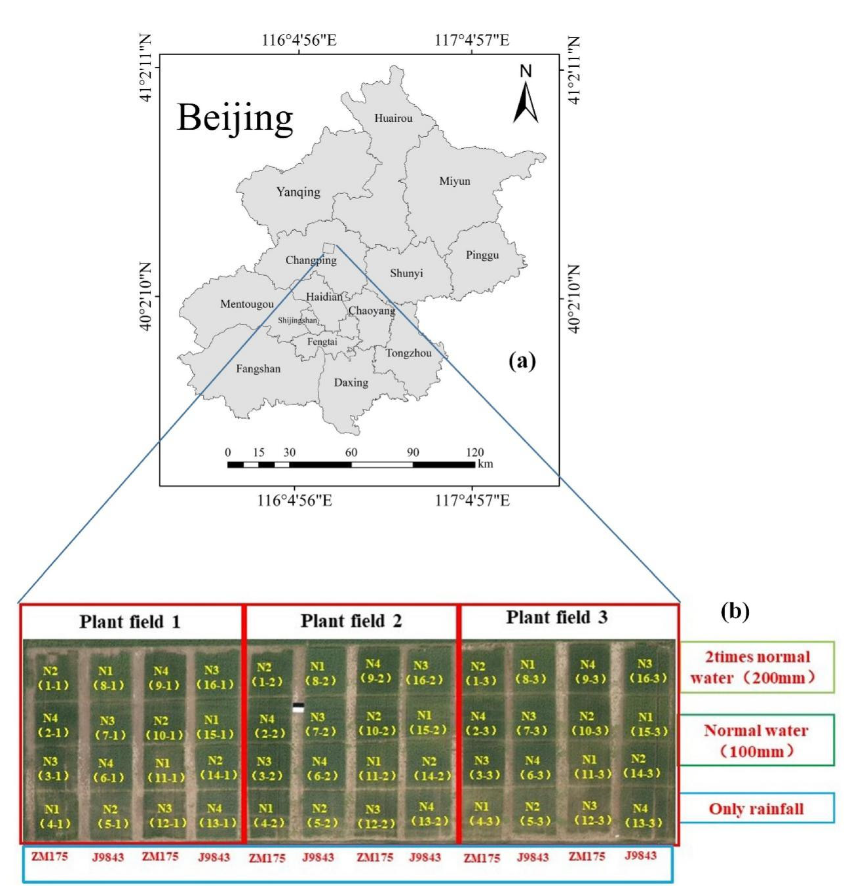
2.1. Survey and Test Design of the Research Area
2.2. Acquisition of Ground Data
2.3. UAV RGB-Data Acquisition and Processing
2.4. UAV Hyperspectral Data Acquisition and Processing
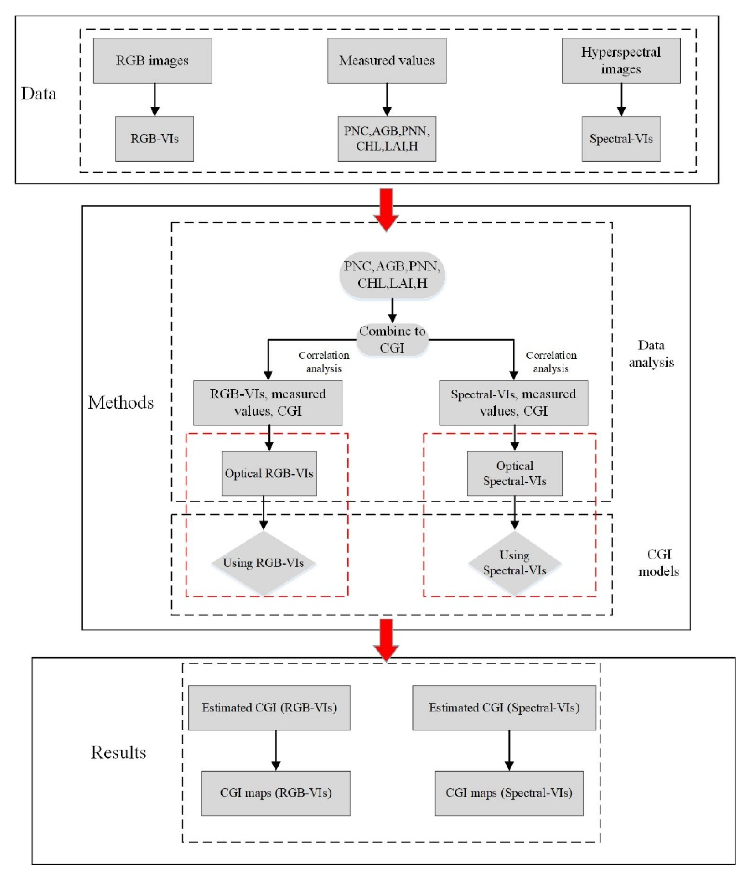
2.5. Research Methods
2.6. Analysis Methods
2.7. Selection of RGB Imagery Indices and Hyperspectral Indices
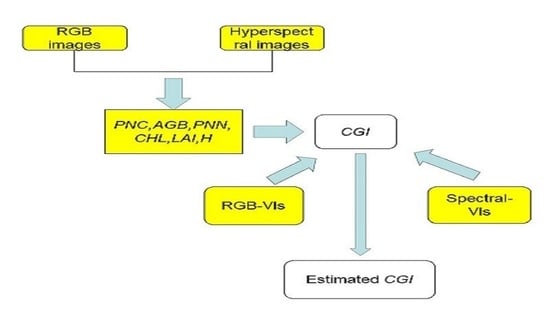
2.8. Construction of Comprehensive Growth Index
2.9. Verification of Accuracy
3. Results and Analysis
3.1. Correlation Analysis
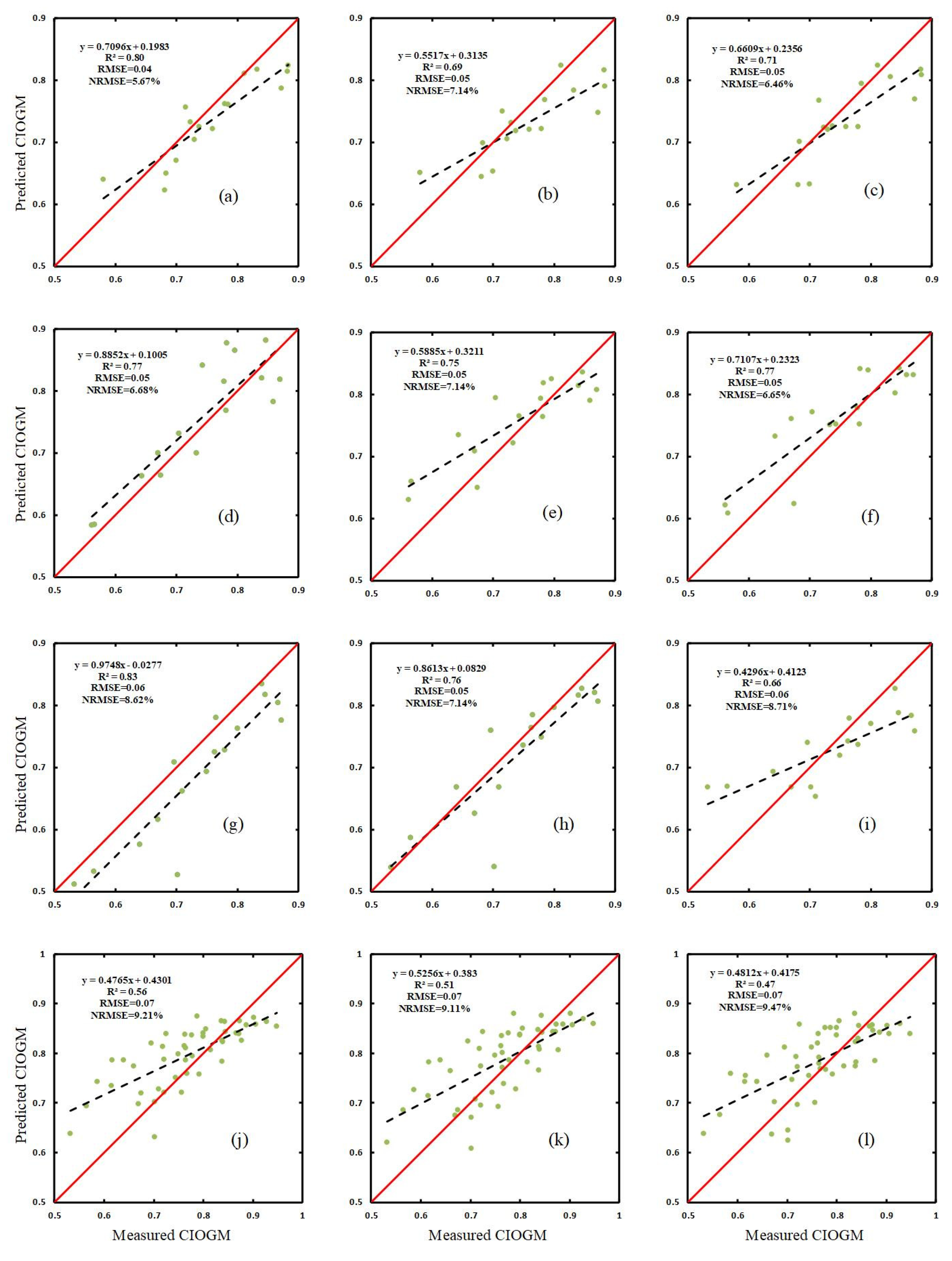
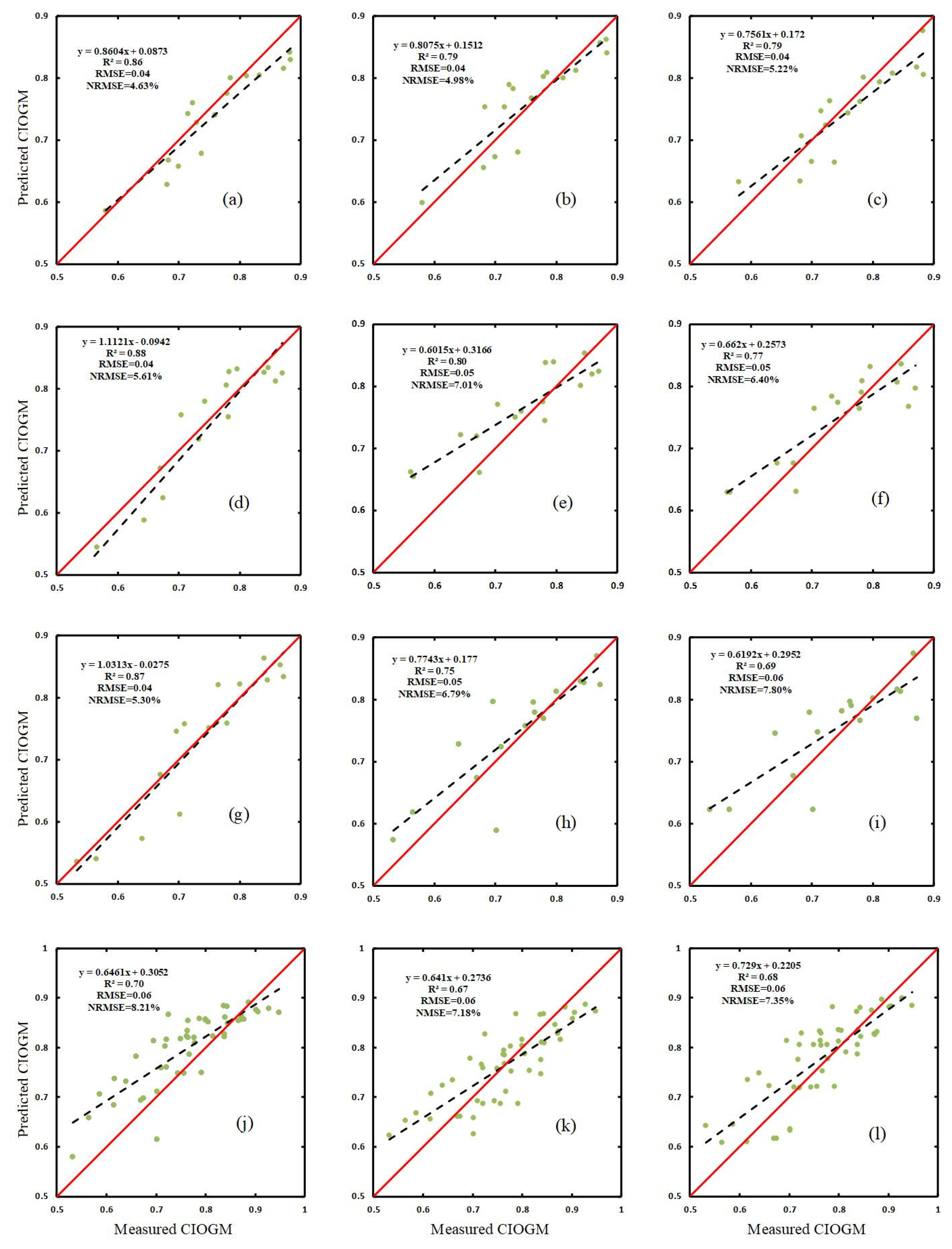
3.2. Estimate of CGI Based on RGB Imagery and Spectral Indices
3.3. Using RGB VIs and Spectral VIs with Machine Learning to Estimate CGI
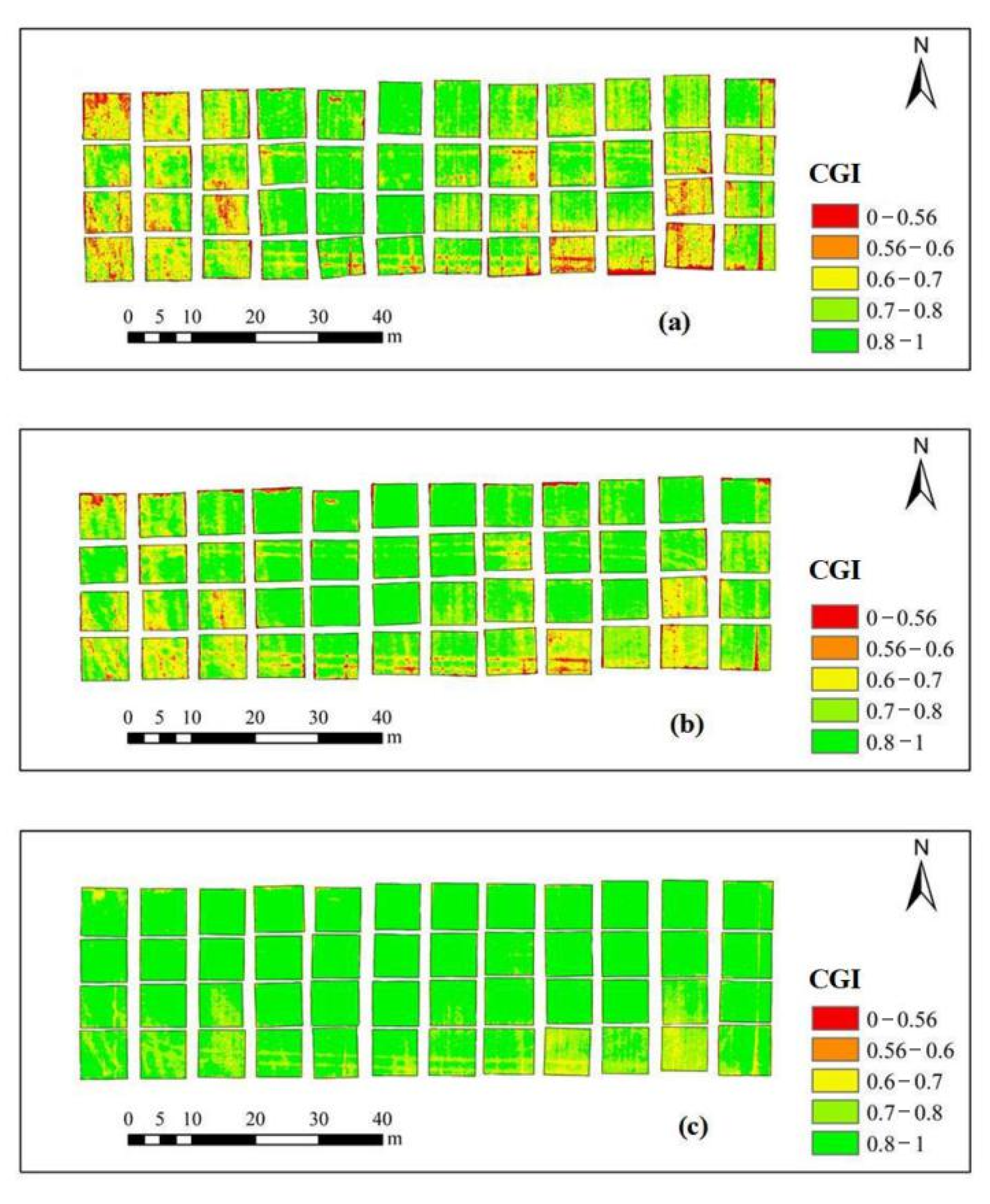
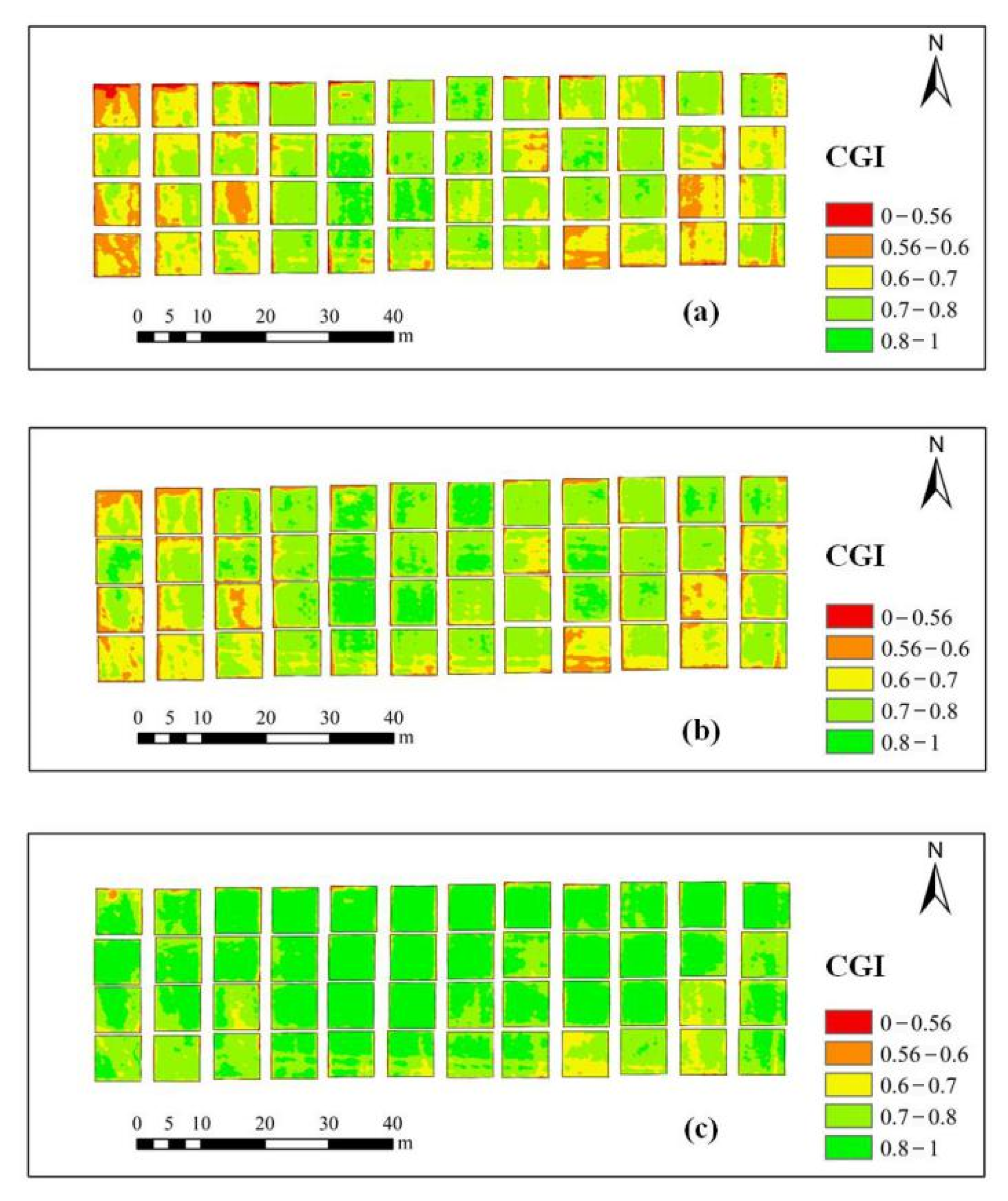
3.4. Map of CGI Distribution
4. Discussion
4.1. Single Growth-Monitoring Indicators and CGI for Winter Wheat
4.2. Estimation of CGI Based on a Single Index
4.3. Estimation of CGI Based on Multiple Indices Combined with Machine Learning
4.4. CGI Estimation Based on Different Sensors
5. Conclusions
Author Contributions
Funding
Acknowledgments
Conflicts of Interest
Abbreviations
| Parameter | Name |
| UAVs | unnamed aerial vehicles |
| CGI | comprehensive growth index |
| MLR | multiple linear regression |
| PLSR | partial least squares |
| RF | random forest |
| PNC | plant nitrogen content |
| AGB | above-ground biomass |
| PWC | plant water content |
| CHL | chlorophyll |
| H | plant height |
References
- Li, X.; Zhang, Y.; Luo, J.; Jin, X.; Xu, Y.; Yang, W. Quantification winter wheat LAI with HJ-1CCD image features over multiple growing seasons. Int. J. Appl. Earth Obs. Geoinf. 2016, 44, 104–112. [Google Scholar] [CrossRef]
- Campos, M.; García, F.J.; Camps, G.; Grau, G.; Nutini, F.; Crema, A.; Boschetti, M. Multitemporal and multiresolution leaf area index retrieval for operational local rice crop monitoring. Remote Sens. Environ. 2016, 187, 102–118. [Google Scholar] [CrossRef]
- Jin, X.; Kumar, L.; Li, Z.; Xu, X.; Yang, G.; Wang, J. Estimation of winter wheat biomass and yield by combining the aquacrop model and field hyperspectral data. Remote Sens. 2016, 8, 972. [Google Scholar] [CrossRef] [Green Version]
- Launay, M.; Guerif, M. Assimilating remote sensing data into a crop model to improve predictive performance for spatial applications. Agric. Ecosyst. Environ. 2005, 111, 321–339. [Google Scholar] [CrossRef]
- Di Gennaro, S.F.; Toscano, P.; Gatti, M.; Poni, S.; Berton, A.; Matese, A. Spectral comparison of UAV-Based hyper and multispectral cameras for precision viticulture. Remote Sens. 2022, 14, 449. [Google Scholar] [CrossRef]
- Berger, K.; Atzberger, C.; Danner, M.; D’Urso, G.; Mauser, W.; Vuolo, F.; Hank, T. Evaluation of the PROSAIL model capabilities for future hyperspectral model environments: A review study. Remote Sens. 2018, 10, 85. [Google Scholar] [CrossRef] [Green Version]
- Taniguchi, K.; Obata, K.; Yoshioka, H. Derivation and approximation of soil isoline equations in the red–near-infrared reflflectance subspace. J. Appl. Remote Sens. 2014, 8, 083621. [Google Scholar] [CrossRef] [Green Version]
- Wang, W.; Gao, X.; Cheng, Y.; Ren, Y.; Zhang, Z.; Wang, R.; Cao, J.; Geng, H. QTL mapping of leaf area index and chlorophyll content based on UAV remote sensing in wheat. EconPapers. 2022, 12, 595. [Google Scholar] [CrossRef]
- Zhang, H.; Tang, Z.; Wang, B.; Meng, B.; Qin, Y.; Sun, Y.; Lv, Y.; Zhang, J.; Yi, S. A non-destructive method for rapid acquisition of grassland aboveground biomass for satellite ground verification using UAV RGB images. Glob. Ecol. Conserv. 2022, 33, e01999. [Google Scholar] [CrossRef]
- Xu, L.; Zhou, L.; Meng, R.; Zhang, F.; Lv, Z.; Xu, B.; Zeng, L.; Yu, X.; Peng, S. An improved approach to estimate ratoon rice aboveground biomass by integrating UAV-based spectral, textural and structural features. Precis. Agric. 2022, 23, 1276–1301. [Google Scholar] [CrossRef]
- Jin, X.; Liu, S.; Baret, F.; Hemerlé, M.; Comar, A. Estimates of plant density of wheat crops at emergence from very low altitude UAV imagery. Remote Sens. Environ. 2017, 198, 105–114. [Google Scholar] [CrossRef] [Green Version]
- Yu, N.; Li, L.; Schmitz, N.; Tian, L.F.; Greenberg, J.A.; Diers, B.W. Development of methods to improve soybean yield estimation and predict plant maturity with an unmanned aerial vehicle based platform. Remote Sens. Environ. 2016, 187, 91–101. [Google Scholar] [CrossRef]
- Maimaitijiang, M.; Ghulam, A.; Sidike, P.; Hartling, S.; Maimaitiyiming, M.; Peterson, K.; Shavers, E.; Fishman, J.; Peterson, J.; Kadam, S.; et al. Unmanned Aerial System (UAS)-based phenotyping of soybean using multi-sensor data fusion and extreme learning machine. ISPRS J. Photogramm. Remote Sens. 2017, 134, 43–58. [Google Scholar] [CrossRef]
- Adar, S.; Sternberg, M.; Paz-Kagan, T.; Henkin, Z.; Dovrat, G.; Zaady, E. Argaman E. Estimation of aboveground biomass production using an unmanned aerial vehicle (UAV) and VENμS satellite imagery in Mediterranean and semiarid rangelands. Remote Sens. Appl. Soc. Environ. 2022, 26, 100753. [Google Scholar]
- Yue, J.; Feng, H.; Jin, X.; Yuan, H.; Li, Z.; Zhou, C.; Yang, G.; Tian, Q. A Comparison of Crop Parameters Estimation Using Images from UAV-Mounted Snapshot Hyperspectral Sensor and High-Definition Digital Camera. Remote Sens. 2018, 10, 1138. [Google Scholar] [CrossRef] [Green Version]
- Geipel, J.; Link, J.; Claupein, W. Combined spectral and spatial modeling of corn yield based on aerial images and crop surface models acquired with an unmanned aircraft system. Remote Sens. 2014, 6, 10335–10355. [Google Scholar] [CrossRef] [Green Version]
- Zaman-Allah, M.; Vergara, O.; Araus, J.; Tarekegne, A.; Magorokosho, C.; Zarco-Tejada, P.; Hornero, A.; Albà, A.; Das, B.; Craufurd, P.; et al. Unmanned aerial platform-based multi-spectral imaging for field phenotyping of maize. Plant Methods 2015, 11, 35. [Google Scholar] [CrossRef] [Green Version]
- Kefauver, S.C.; Vicente, R.; Vergara-Diaz, O.; Fernandez-Gallego, J.A.; Serret, M.M.D.; Araus, J.L.; Kerfal, S.; Lopez, A.; Melichar, J.P.E. Comparative UAV and field phenotyping to assess yield and nitrogen use efficiency in hybrid and conventional barley. Front. Plant Sci. 2017, 8, 1733. [Google Scholar] [CrossRef]
- Chen, P.; Li, G.; Shi, Y.; Xu, Z.; Yang, F.; Cao, Q. Validation of an unmanned aerial vehicle hyperspectral sensor and its application in maize leaf area index estimation. Sci. Agric. Sin. 2018, 51, 1464–1474. [Google Scholar]
- Han, L.; Yang, G.; Dai, H.; Xu, B.; Yang, H.; Feng, H.; Li, Z.; Yang, X. Modeling maize above-ground biomass based on machine learning approaches using UAV remote-sensing data. Plant Methods 2019, 15, 10. [Google Scholar] [CrossRef] [Green Version]
- Swain, K.; Thomson, S.; Jayasuriya, H. Adoption of an Unmanned Helicopter for Low-Altitude Remote Sensing to Estimate Yield and Total Biomass of a Rice Crop. Trans. ASABE 2010, 53, 21–27. [Google Scholar] [CrossRef] [Green Version]
- Chang, X.; Chang, Q.; Wang, X.; Chu, D.; Guo, R. Estimation of maize leaf chlorophyll contents based on UAV hyperspectral drone image. Agric. Res. Arid. Areas 2019, 37, 66–73. [Google Scholar]
- Schirrmann, M.; Giebel, A.; Gleiniger, F.; Pflanz, M.; Lentschke, J.; Dammer, K.-H. Monitoring agronomic parameters of winter wheat crops with low-cost UAV imagery. Remote Sens. 2016, 8, 706. [Google Scholar] [CrossRef] [Green Version]
- Li, Z.; Nie, C.; Wei, C.; Xu, X.; Song, X.; Wang, J. Comparison of four chemometric techniques for estimating leaf nitrogen concentrations in winter wheat (Triticum aestivum) based on hyperspectral features. J. Appl. Spectrosc. 2016, 83, 240–247. [Google Scholar] [CrossRef]
- Duan, S.; Li, Z.; Wu, H.; Tang, B.; Ma, L.; Zhao, E.; Li, C. Inversion of the PROSAIL model to estimate leaf area index of maize, potato, and sunflower fields from unmanned aerial vehicle hyperspectral data. Int. J. Appl. Earth Obs. Geoinf. 2014, 26, 12–20. [Google Scholar] [CrossRef]
- Li, J.; Zhu, X.; Ma, L.; Zhao, Y.; Qian, Y.; Tang, L. Leaf Area Index Retrieval and Scale Effect Analysis of Multiple Crops from UAV-based Hyperspectral Data. Remote Sens. Technol. Appl. 2017, 32, 427–434. [Google Scholar]
- Lucieer, A.; Malenovsky, Z.; Veness, T.; Wallace, L. HyperUAS-imaging spectroscopy from a multirotor unmanned aircraft system. J. Field Robot. 2014, 31, 571–590. [Google Scholar] [CrossRef] [Green Version]
- Turner, D.; Lucieer, A.; Wallace, L. Direct Georeferencing of Ultrahigh-Resolution UAV Imagery. IEEE Trans. Geosci. Remote Sens. 2014, 52, 2738–2745. [Google Scholar] [CrossRef]
- Darvishzadeh, R.; Skidmore, A.; Schlerf, M.; Atzberger, C.; Corsi, F.; Cho, M. Lai and chlorophyll estimation for a heterogeneous grassland using hyperspectral measurements. ISPRS J. Photogramm. Remote Sens. 2008, 63, 409–426. [Google Scholar] [CrossRef]
- Kuangnan, F.; Jianbin, W.; Jianping, Z.; Bangchang, X. A review of technologies on random forests. Stat. Inf. Forum 2011, 26, 32–38. [Google Scholar]
- Breiman, L. Random Forests. Mach. Learn. 2001, 45, 5–32. [Google Scholar] [CrossRef] [Green Version]
- Yue, J.; Feng, H.; Yang, G.; Li, Z. A comparison of regression techniques for estimation of above-ground winter wheat biomass using near-surface spectroscopy. Remote Sens. 2018, 10, 66. [Google Scholar] [CrossRef] [Green Version]
- Atzberger, C.; Darvishzadeh, R.; Immitzer, M.; Schlerf, M.; Skidmore, A.; le Maire, G. Comparative analysis of different retrieval methods for mapping grassland leaf area index using airborne imaging spectroscopy. Int. J. Appl. Earth Obs. Geoinf. 2015, 43, 19–31. [Google Scholar] [CrossRef] [Green Version]
- Gitelson, A.; Kaufman, Y.; Stark, R.; Rundquist, D. Novel algorithms for remote estimation of vegetation fraction. Remote Sens. Environ. 2002, 80, 76–87. [Google Scholar] [CrossRef] [Green Version]
- Bendig, J.; Yu, K.; Aasen, H.; Bolten, A.; Bennertz, S.; Broscheit, J.; Gnyp, M.; Bareth, G. Combining UAV-based plant height from crop surface models, visible, and near infrared vegetation indices for biomass monitoring in barley. Int. J. Appl. Earth Obs. Geoinf. 2015, 39, 79–87. [Google Scholar] [CrossRef]
- Kataoka, T.; Kaneko, T.; Okamoto, H.; Hata, S. Crop growth estimation system using machine vision. In Proceedings of the IEEE/ASME International Conference on Advanced Intelligent Mechatronics, Kobe, Japan, 20–24 July 2003; pp. 1079–1083. [Google Scholar]
- Torressnchez, J. Multi-temporal mapping of the vegetation fraction in early-season wheat fields using images from UAV. Comput. Electron. Agric. 2014, 103, 104–113. [Google Scholar] [CrossRef]
- Chianucci, F.; Disperati, L.; Guzzi, D.; Bianchini, D.; Nardino, V.; Lastri, C.; Rindinella, A.; Corona, P. Estimation of canopy attributes in beech forests using true colour digital images from a small fixed-wing UAV. Int. J. Appl. Earth Obs. Geoinf. 2016, 47, 60–68. [Google Scholar] [CrossRef] [Green Version]
- Penuelas, J.; Isla, R.; Filella, I.; Araus, J. Visible and near-infrared reflectance assessment of salinity effects on barley. Crop Sci. 1997, 37, 198–202. [Google Scholar] [CrossRef]
- Baret, F.; Guyot, G.; Major, D.J. TSAVI: A vegetation index which minimizes soil brightness effects on LAI and APAR estimation. Symp. Remote Sens. Geosci. Remote Sens. Symp. 1989, 3, 1355–1358. [Google Scholar]
- Wu, C.; Niu, Z.; Tang, Q.; Huang, W. Estimating chlorophyll content from hyperspectral vegetation indices: Modeling and validation. Agric. For. Meteorol. 2008, 148, 1230–1241. [Google Scholar] [CrossRef]
- Haboudane, D.; Miller, J.R.; Tremblay, N.; Zarco-Tejada, P.J.; Dextraze, L. Integrated narrow-band vegetation indices for prediction of crop chlorophyll content for application to precision agriculture. Remote Sens. Environ. 2002, 81, 416–426. [Google Scholar] [CrossRef]
- Huete, A. A Modified soil adjusted vegetation index. Remote Sens. Environ. 1994, 48, 119–126. [Google Scholar]
- Vincini, M.; Frazzi, E. Angular dependence of maize and sugar beet VIs from directional CHRIS/Proba data. Cuore 2005, 2, 5–9. [Google Scholar]
- Datt, B. A new reflectance index for remote sensing of chlorophyll content in higher plants: Tests using Eucalyptus leaves. J. Plant Physiol. 1999, 154, 30–36. [Google Scholar] [CrossRef]
- Roujean, J.L.; Breon, F.M. Estimating PAR absorbed by vegetation from bidirectional reflectance measurements. Remote Sens. Environ. 1995, 51, 375–384. [Google Scholar] [CrossRef]
- Zarco-Tejada, P.J.; Berjón, A.; López-Lozano, R.; Miller, J.R.; Martín, P.; Cachorro, V.; González, M.R.; De Frutos, A. Assessing vineyard condition with hyperspectral indices: Leaf and canopy reflflectance simulation in a row-structured discontinuous canopy. Remote Sens. Environ. 2005, 99, 271–287. [Google Scholar] [CrossRef]
- Peñuelas, J.; Gamon, J.A.; Fredeen, A.L.; Merino, J.; Field, C.B. Reflectance indices associated with physiological changes in nitrogen- and water-limited sunflower leaves. Remote Sens. Environ. 1994, 48, 135–146. [Google Scholar] [CrossRef]
- Zhou, X.; Zheng, H.B.; Xu, X.Q.; He, J.Y.; Ge, X.K.; Yao, X.; Cheng, T.; Zhu, Y.; Cao, Y.X.; Tian, Y.C. Predicting grain yield in rice using multi-temporal vegetation indices from UAV-based multispectral and digital imagery. ISPRS J. Photogramm. Remote Sens. 2017, 130, 246–255. [Google Scholar] [CrossRef]
- Niu, Q.; Feng, H.; Yang, G.; Yang, H.; Xu, B.; Zhao, Y. Monitoring plant height and leaf area index of maize breeding material based on UAV digital images. Nongye Gongcheng Xuebao/Trans. Chin. Soc. Agric. Eng. 2018, 34, 73–82. [Google Scholar]
- Liang, L.; Di, L.; Zhang, L.; Deng, M.; Qin, Z.; Zhao, S.; Lin, H. Estimation of crop LAI using hyperspectral vegetation indices and a hybrid inversion method. Remote Sens. Environ. 2015, 165, 123–134. [Google Scholar] [CrossRef]
- Zhu, H.; Liu, H.; Xu, Y.; Yang, G. UAV-based hyperspectral analysis and spectral indices constructing for quantitatively monitoring leaf nitrogen content of winter wheat. Appl. Opt. 2018, 57, 7722–7732. [Google Scholar] [CrossRef] [PubMed]
- Nguy-Robertson, A.; Gitelson, A.; Peng, Y.; Viña, A.; Arkebauer, T.; Rundquist, D. Green leaf area index estimation in maize and soybean: Combining vegetation indices to achieve maximal sensitivity. Agron. J. 2012, 104, 1336–1347. [Google Scholar] [CrossRef] [Green Version]
- Yue, J.; Yang, G.; Li, C.; Li, Z.; Wang, Y.; Feng, H.; Xu, B. Estimation of Winter Wheat Above-Ground Biomass Using Unmanned Aerial Vehicle-Based Snapshot Hyperspectral Sensor and Crop Height Improved Models. Remote Sens. 2017, 9, 708. [Google Scholar] [CrossRef] [Green Version]
- Ozlem, A. Mapping land use with using Rotation Forest algorithm from UAV images. Eur. J. Remote Sens. 2017, 50, 269–279. [Google Scholar]
- Knyazikhin, Y.; Schull, M.A.; Stenberg, P.; Mõttus, M.; Rautiainen, M.; Yang, Y.; Marshak, A.; Carmona, P.L.; Kaufmann, R.K.; Lewis, P.; et al. Hyperspectral remote sensing of foliar nitrogen content. Proc. Natl. Acad. Sci. USA 2013, 110, 811–812. [Google Scholar] [CrossRef] [Green Version]
- Knyazikhin, Y.; Lewis, P.; Disney, M.I.; Mottus, M.; Rautiainen, M.; Stenberg, P.; Kaufmann, R.K.; Marshak, A.; Schull, M.A.; Carmona, P.L.; et al. Reply to Ollinger et al.: Remote sensing of leaf nitrogen and emergent ecosystem properties. Proc. Natl. Acad. Sci. USA 2013, 110, 2438. [Google Scholar] [CrossRef] [Green Version]
- Ollinger, S.V.; Richardson, A.D.; Martin, M.E.; Hollinger, D.Y.; Frolking, S.E.; Reich, P.B.; Plourde, L.C.; Katul, G.G.; Munger, J.W.; Oren, R.; et al. Canopy nitrogen, carbon assimilation, and albedo in temperate and boreal forests: Functional relations and potential climate feedbacks. Proc. Natl. Acad. Sci. USA 2008, 105, 19336–19341. [Google Scholar] [CrossRef] [Green Version]
- Knyazikhin, Y.; Lewis, P.; Disney, M.I.; Stenberg, P.; Mõttus, M.; Rautiainen, M.; Kaufmann, R.K.; Marshak, A.; Schull, M.A.; Carmona, P.L.; et al. Reply to Townsend et al.: Decoupling contributions from canopy structure and leaf optics is critical for remote sensing leaf biochemistry. Proc. Natl. Acad. Sci. USA 2013, 110, 1075. [Google Scholar] [CrossRef] [Green Version]
- Townsend, P.A.; Serbin, S.P.; Kruger, E.L.; Gamon, J.A. Disentangling the contribution of biological and physical properties of leaves and canopies in imaging spectroscopy data. Proc. Natl. Acad. Sci. USA 2013, 110, 1074. [Google Scholar] [CrossRef] [Green Version]
- Dashti, H.; Glenn, N.F.; Ustin, S.; Mitchell, J.J.; Qi, Y.; Ilangakoon, N.T.; Flores, A.N.; Silván-Cárdenas, J.L.; Zhao, K.; Spaete, L.P.; et al. Empirical Methods for Remote Sensing of Nitrogen in Drylands May Lead to Unreliable Interpretation of Ecosystem Function. IEEE Trans. Geosci. Remote Sens. 2019, 57, 3993–4004. [Google Scholar] [CrossRef]
- Bendig, J.; Bolten, A.; Bennertz, S.; Broscheit, J.; Eichfuss, S.; Bareth, G. Estimating biomass of barley using crop surface models (CSMs) derived from UAV-based RGB imaging. Remote Sens. 2014, 6, 10395–10412. [Google Scholar] [CrossRef] [Green Version]
- Rasmussen, J.; Ntakos, G.; Nielsen, J.; Svensgaard, J.; Christensen, S.; Poulsen, R.N. Are vegetation indices derived from consumer-grade cameras mounted on UAVs sufficiently reliable for assessing experimental plots? Eur. J. Agron. 2016, 74, 75–92. [Google Scholar] [CrossRef]

| Type | Index | Formula | References |
|---|---|---|---|
| RGB-imagery-based vegetation indices | R | R = R | [15] |
| G | G = G | [15] | |
| B | B = B | [15] | |
| r | r = R/(R + G + B) | [15] | |
| g | g = G/(R + G + B) | [15] | |
| b | b = B/(R + G + B) | [15] | |
| EXR | EXR = 1.4 r − g | [33] | |
| VARI | VARI = (g − r)/(g + r − b) | [34] | |
| GRVI | GRVI = (g − r)/(g + r) | [35] | |
| MGRVI | MGRVI = (g2 − r2)/(g2 + r2) | [35] | |
| CIVE | CIVE = 0.441 r − 0.881 g + 0.385 b + 18.78745 | [36] | |
| EXG | EXG = 2 g − b − r | [37] | |
| GLA | GLA = (2G – B − R)/(2G + B + R) | [38] | |
| Hyperspectral-imagery-based vegetation indices | NDVI | (R800 − R680)/(R800 + R680) | [39] |
| SR | R750/R550 | [40] | |
| MSR | (R800/R760 − 1)/(R800/R670 + 1)1/2 | [41] | |
| MCARI | ((R700 − R670) − 0.2 × (R700 − R550))(R700/R670) | [42] | |
| TCARI | 3[(R700 − R670) − 0.2(R700 − R550)(R700/R670)] | [42] | |
| MSAVI | 0.5[2R800 + 1 − ((2R800 + 1)2 − 8(R800 − R670))1/2] | [43] | |
| OSAVI | 1.16 × (R800 − R670)/(R800 + R670 + 0.16) | [8] | |
| EVI2 | 2.5 × (R800 − R670)/(R800 + 2.4 × R670 + 1) | [9] | |
| SPVI | 0.4[3.7(R800 − R670) − 1.2|R530 − R670|] | [44] | |
| LCI | (R850 − R710)/(R850 + R680) | [45] | |
| RDVI | (R800 − R670)/(R800 + R670)1/2 | [46] | |
| BGI | R460/R560 | [47] | |
| NPCI | (R670 − R460)/(R670 + R460) | [48] |
| Stages | Index | Correlation Coefficient | ||||||
|---|---|---|---|---|---|---|---|---|
| PNC | AGB | PWC | CHL | LAI | H | CGI | ||
| (GS 31) | R | −0.56 ** | −0.72 ** | −0.66 ** | −0.65 ** | −0.78 ** | −0.50 ** | −0.85 ** |
| r | −0.72 ** | −0.61 ** | −0.69 ** | −0.69 ** | −0.65 ** | −0.50 ** | −0.81 ** | |
| EXR | −0.64 ** | −0.63 ** | −0.63 ** | −0.65 ** | −0.69 ** | −0.51 ** | −0.81 ** | |
| G | −0.47 ** | −0.72 ** | −0.64 ** | −0.59 ** | −0.78 ** | −0.46 ** | −0.80 ** | |
| VARI | 0.63 ** | 0.63 ** | 0.62 ** | 0.64 ** | 0.69 ** | 0.52 ** | 0.80 ** | |
| MGRVI | 0.63 ** | 0.63 ** | 0.61 ** | 0.64 ** | 0.69 ** | 0.52 ** | 0.80 ** | |
| GRVI | 0.63 ** | 0.63 ** | 0.61 ** | 0.64 ** | 0.69 ** | 0.52 ** | 0.80 ** | |
| B | −0.35 * | −0.69 ** | −0.52 ** | −0.50 ** | −0.76 ** | −0.45 ** | −0.73 ** | |
| CIVE | −0.47 ** | −0.61 ** | −0.49 ** | −0.52 ** | −0.69 ** | −0.49 ** | −0.72 ** | |
| GLA | 0.45 ** | 0.60 ** | 0.48 ** | 0.51 ** | 0.68 ** | 0.49 ** | 0.71 ** | |
| EXG | 0.45 ** | 0.60 ** | 0.48 ** | 0.51 ** | 0.68 ** | 0.49 ** | 0.71 ** | |
| g | 0.45 ** | 0.60 ** | 0.48 ** | 0.51 ** | 0.68 ** | 0.49 ** | 0.71 ** | |
| b | 0.66 ** | 0.23 | 0.54 ** | 0.51 ** | 0.18 | 0.19 | 0.43 ** | |
| (GS 47) | R | −0.51 ** | −0.68 ** | −0.66 ** | −0.45 ** | −0.63 ** | −0.48 ** | −0.69 ** |
| r | −0.64 ** | −0.73 ** | −0.68 ** | −0.53 ** | −0.74 ** | −0.70 ** | −0.81 ** | |
| EXR | −0.56 ** | −0.71 ** | −0.69 ** | −0.43 ** | −0.72 ** | −0.72 ** | −0.77 ** | |
| G | −0.41 ** | −0.57 ** | −0.56 ** | −0.41 ** | −0.49 ** | −0.23 | −0.55 ** | |
| VARI | 0.55 ** | 0.70 ** | 0.69 ** | 0.42 ** | 0.72 ** | 0.72 ** | 0.76 ** | |
| MGRVI | 0.53 ** | 0.70 ** | 0.69 ** | 0.40 ** | 0.71 ** | 0.73 ** | 0.75 ** | |
| GRVI | 0.53 ** | 0.70 ** | 0.69 ** | 0.40 ** | 0.71 ** | 0.73 ** | 0.75 ** | |
| B | −0.13 | −0.40 ** | −0.47 ** | −0.11 | −0.32 | −0.13 | −0.31 * | |
| CIVE | −0.24 | −0.53 ** | −0.62 ** | −0.08 | −0.56 ** | −0.68 ** | −0.52 ** | |
| GLA | 0.20 | 0.50 ** | 0.60 ** | 0.03 | 0.53 ** | 0.66 ** | 0.48 ** | |
| EXG | 0.20 | 0.50 ** | 0.60 ** | 0.03 | 0.53 ** | 0.66 ** | 0.48 ** | |
| g | 0.20 | 0.50 ** | 0.60 ** | 0.03 | 0.53 ** | 0.66 ** | 0.48 ** | |
| b | 0.76 ** | 0.70 ** | 0.56 ** | 0.72 ** | 0.69 ** | 0.56 ** | 0.83 ** | |
| (GS 65) | R | −0.40 ** | −0.63 ** | −0.67 ** | −0.41 ** | −0.63 ** | −0.48 ** | −0.79 ** |
| r | −0.49 ** | −0.71 ** | −0.79 ** | −0.45 ** | −0.74 ** | −0.72 ** | −0.81 ** | |
| EXR | −0.37 ** | −0.69 ** | −0.72 ** | −0.35 * | −0.68 ** | −0.71 ** | −0.79 ** | |
| G | −0.39 ** | −0.51 ** | −0.55 ** | −0.42 ** | −0.51 ** | −0.20 | −0.67 ** | |
| VARI | 0.37 ** | 0.69 ** | 0.72 ** | 0.35 * | 0.69 ** | 0.71 ** | 0.80 ** | |
| MGRVI | 0.35 * | 0.68 ** | 0.71 ** | 0.33 * | 0.67 ** | 0.70 ** | 0.79 ** | |
| GRVI | 0.35 * | 0.68 ** | 0.71 ** | 0.33 * | 0.67 ** | 0.70 ** | 0.79 ** | |
| B | −0.14 | −0.43 ** | −0.39 ** | −0.20 | −0.39 ** | −0.22 | −0.59 ** | |
| CIVE | −0.13 | −0.59 ** | −0.54 ** | −0.16 | −0.54 ** | −0.63 ** | −0.69 ** | |
| GLA | 0.11 | 0.57 ** | 0.52 ** | 0.15 | 0.52 ** | 0.62 ** | 0.68 ** | |
| EXG | 0.11 | 0.57 ** | 0.52 ** | 0.15 | 0.52 ** | 0.62 ** | 0.68 ** | |
| g | 0.11 | 0.57 ** | 0.52 ** | 0.15 | 0.52 ** | 0.62 ** | 0.68 ** | |
| b | 0.78 ** | 0.52 ** | 0.75 ** | 0.64 ** | 0.64 ** | 0.46 ** | 0.56 ** | |
| Total for three stages | R | −0.47 ** | −0.64 ** | −0.63 ** | −0.48 ** | −0.51 ** | −0.50 ** | −0.68 ** |
| r | −0.64 ** | −0.65 ** | −0.27 ** | −0.45 ** | −0.46 ** | −0.68 ** | −0.71 ** | |
| EXR | −0.55 ** | −0.67 ** | −0.42 ** | −0.44 ** | −0.57 ** | −0.67 ** | −0.74 ** | |
| G | −0.36 ** | −0.53 ** | −0.65 ** | −0.42 ** | −0.40 ** | −0.32 ** | −0.55 ** | |
| VARI | 0.54 ** | 0.68 ** | 0.42 ** | 0.43 ** | 0.57 ** | 0.68 ** | 0.74 ** | |
| MGRVI | 0.53 ** | 0.67 ** | 0.44 ** | 0.43 ** | 0.58 ** | 0.66 ** | 0.73 ** | |
| GRVI | 0.53 ** | 0.67 ** | 0.44 ** | 0.43 ** | 0.58 ** | 0.66 ** | 0.73 ** | |
| B | −0.07 | −0.36 ** | −0.69 ** | −0.24 ** | −0.36 * | −0.15 | −0.36 ** | |
| CIVE | −0.19 * | −0.50 ** | −0.59 ** | −0.28 ** | −0.57 ** | −0.44 ** | −0.55 ** | |
| GLA | 0.5 | 0.47 ** | 0.59 ** | 0.25 ** | 0.55 ** | 0.41 ** | 0.52 ** | |
| EXG | 0.15 | 0.47 ** | 0.59 ** | 0.25 ** | 0.56 ** | 0.41 ** | 0.52 ** | |
| g | 0.15 | 0.47 ** | 0.59 ** | 0.25 ** | 0.56 ** | 0.41 ** | 0.52 ** | |
| b | 0.61 ** | 0.41 ** | −0.11 | 0.33 ** | 0.15 | 0.48 ** | 0.44 ** | |
| Stages | Index | Correlation Coefficient | ||||||
|---|---|---|---|---|---|---|---|---|
| PNC | AGB | PWC | CHL | LAI | H | CGI | ||
| (GS 31) | LCI | 0.62 ** | 0.67 ** | 0.65 ** | 0.75 ** | 0.70 ** | 0.48 ** | 0.83 ** |
| MSR | 0.63 ** | 0.64 ** | 0.63 ** | 0.69 ** | 0.66 ** | 0.48 ** | 0.80 ** | |
| SR | 0.64 ** | 0.63 ** | 0.65 ** | 0.67 ** | 0.65 ** | 0.49 ** | 0.79 ** | |
| NDVI | 0.57 ** | 0.62 ** | 0.57 ** | 0.70 ** | 0.65 ** | 0.45 ** | 0.77 ** | |
| NPCI | −0.68 ** | −0.58 ** | −0.63 ** | −0.67 ** | −0.62 ** | −0.42 ** | −0.77 ** | |
| OSAVI | 0.52 ** | 0.44 ** | 0.42 ** | 0.66 ** | 0.49 ** | 0.32 * | 0.62 ** | |
| BGI | 0.57 ** | 0.45 ** | 0.70 ** | 0.49 ** | 0.45 ** | 0.26 | 0.58 ** | |
| RDVI | 0.49 ** | 0.37 ** | 0.35 * | 0.61 ** | 0.42 ** | 0.27 | 0.54 ** | |
| EVI2 | 0.45 ** | 0.30 * | 0.30 * | 0.56 ** | 0.35 * | 0.22 | 0.47 ** | |
| MSAVI | 0.45 ** | 0.29 * | 0.30 * | 0.56 ** | 0.35 * | 0.23 | 0.47 ** | |
| SPVI | 0.38 ** | 0.20 | 0.21 | 0.49 ** | 0.25 | 0.15 | 0.36 ** | |
| TCARI | −0.12 | −0.31 * | −0.42 ** | −0.09 | −0.28 | −0.27 | −0.29 * | |
| MCARI | 0.19 | 0.01 | −0.07 | 0.22 | 0.06 | 0.02 | 0.11 | |
| (GS 47) | LCI | 0.68 ** | 0.78 ** | 0.64 ** | 0.60 ** | 0.74 ** | 0.69 ** | 0.85 ** |
| MSR | 0.63 ** | 0.76 ** | 0.62 ** | 0.51 ** | 0.73 ** | 0.73 ** | 0.82 ** | |
| NDVI | 0.63 ** | 0.76 ** | 0.58 ** | 0.53 ** | 0.70 ** | 0.74 ** | 0.81 ** | |
| SR | 0.62 ** | 0.75 ** | 0.63 ** | 0.49 ** | 0.73 ** | 0.72 ** | 0.81 ** | |
| OSAVI | 0.67 ** | 0.74 ** | 0.46 ** | 0.51 ** | 0.68 ** | 0.79 ** | 0.81 ** | |
| NPCI | −0.61 ** | −0.75 ** | −0.65 ** | −0.49 ** | −0.71 ** | −0.71 ** | −0.80 ** | |
| RDVI | 0.68 ** | 0.70 ** | 0.39 ** | 0.49 ** | 0.66 ** | 0.80 ** | 0.78 ** | |
| MSAVI | 0.67 ** | 0.70 ** | 0.38 ** | 0.48 ** | 0.65 ** | 0.80 ** | 0.78 ** | |
| EVI2 | 0.67 ** | 0.69 ** | 0.36 * | 0.47 ** | 0.64 ** | 0.80 ** | 0.77 ** | |
| SPVI | 0.66 ** | 0.63 ** | 0.28 | 0.44 ** | 0.60 ** | 0.79 ** | 0.72 ** | |
| BGI | 0.58 ** | 0.65 ** | 0.67 ** | 0.54 ** | 0.61 ** | 0.44 ** | 0.71 ** | |
| TCARI | −0.24 | −0.37 ** | −0.61 ** | −0.38 ** | −0.37 ** | 0.01 | −0.38 ** | |
| MCARI | 0.06 | 0.05 | −0.26 | −0.16 | 0.01 | 0.45 ** | 0.05 | |
| (GS 65) | LCI | 0.55 ** | 0.77 ** | 0.79 ** | 0.53 ** | 0.78 ** | 0.66 ** | 0.84 ** |
| MSAVI | 0.48 ** | 0.80 ** | 0.75 ** | 0.41 ** | 0.77 ** | 0.79 ** | 0.83 ** | |
| SPVI | 0.48 ** | 0.80 ** | 0.74 ** | 0.41 ** | 0.77 ** | 0.80 ** | 0.83 ** | |
| EVI2 | 0.48 ** | 0.79 ** | 0.75 ** | 0.42 ** | 0.77 ** | 0.79 ** | 0.82 ** | |
| RDVI | 0.48 ** | 0.78 ** | 0.76 ** | 0.43 ** | 0.76 ** | 0.79 ** | 0.82 ** | |
| SR | 0.45 ** | 0.81 ** | 0.78 ** | 0.40 ** | 0.80 ** | 0.69 ** | 0.82 ** | |
| MSR | 0.46 ** | 0.80 ** | 0.79 ** | 0.42 ** | 0.78 ** | 0.71 ** | 0.82 ** | |
| OSAVI | 0.48 ** | 0.77 ** | 0.77 ** | 0.44 ** | 0.76 ** | 0.77 ** | 0.82 ** | |
| NDVI | 0.45 ** | 0.73 ** | 0.76 ** | 0.44 ** | 0.72 ** | 0.71 ** | 0.77 ** | |
| BGI | 0.61 ** | 0.71 ** | 0.62 ** | 0.61 ** | 0.69 ** | 0.42 ** | 0.77 ** | |
| NPCI | −0.40 ** | −0.75 ** | −0.76 ** | −0.38 ** | −0.72 ** | −0.74 ** | −0.76 ** | |
| MCARI | −0.05 | 0.49 ** | 0.45 ** | −0.03 | 0.40 ** | 0.81 ** | 0.40 ** | |
| TCARI | −0.20 | 0.20 | 0.19 | −0.20 | 0.12 | 0.72 ** | 0.14 | |
| Total for three stages | LCI | 0.63 ** | 0.74 ** | 0.40 ** | 0.60 ** | 0.65 ** | 0.60 ** | 0.82 ** |
| MSR | 0.58 ** | 0.74 ** | 0.52 ** | 0.52 ** | 0.63 ** | 0.65 ** | 0.80 ** | |
| SR | 0.58 ** | 0.74 ** | 0.52 ** | 0.50 ** | 0.63 ** | 0.64 ** | 0.80 ** | |
| NDVI | 0.55 ** | 0.69 ** | 0.50 ** | 0.54 ** | 0.59 ** | 0.62 ** | 0.76 ** | |
| OSAVI | 0.54 ** | 0.63 ** | 0.54 ** | 0.49 ** | 0.48 ** | 0.62 ** | 0.70 ** | |
| NPCI | −0.55 ** | −0.65 ** | −0.51 ** | −0.41 ** | −0.40 ** | −0.67 ** | −0.67 ** | |
| RDVI | 0.52 ** | 0.58 ** | 0.54 ** | 0.46 ** | 0.42 ** | 0.61 ** | 0.65 ** | |
| MSAVI | 0.50 ** | 0.56 ** | 0.53 ** | 0.43 ** | 0.39 ** | 0.59 ** | 0.62 ** | |
| EVI2 | 0.50 ** | 0.55 ** | 0.53 ** | 0.43 ** | 0.38 ** | 0.59 ** | 0.62 ** | |
| SPVI | 0.46 ** | 0.49 ** | 0.51 ** | 0.38 ** | 0.32 ** | 0.55 ** | 0.55 ** | |
| BGI | 0.50 ** | 0.49 ** | 0.43 ** | 0.33 ** | 0.15 | 0.47 ** | 0.48 ** | |
| TCARI | −0.11 | −0.13 | 0.23 ** | −0.16 | −0.28 ** | 0.13 | −0.16 | |
| MCARI | 0.07 | 0.13 | 0.39 ** | 0.01 | −0.05 | 0.34 ** | 0.12 | |
| Growth Stages | Parameters | Equations | Calibration | Verification | ||||
|---|---|---|---|---|---|---|---|---|
| R2 | RMSE | NRMSE (%) | R2 | RMSE | NRMSE (%) | |||
| (GS 31) | r | y = 8.7269 × e−6.874x | 0.67 | 0.05 | 6.55 | 0.78 | 0.04 | 4.98 |
| EXR | y = 1.0729 × e−3.196x | 0.65 | 0.05 | 6.73 | 0.73 | 0.04 | 5.49 | |
| VARI | y = 0.6664 × e1.8637x | 0.64 | 0.05 | 6.78 | 0.72 | 0.04 | 5.58 | |
| MGRVI | y = 0.6655 × e1.449x | 0.64 | 0.05 | 6.79 | 0.71 | 0.04 | 5.66 | |
| LCI | y = 0.3945 × e1.067x | 0.72 | 0.04 | 5.92 | 0.74 | 0.04 | 5.38 | |
| MSR | y = 0.5264 × e0.1375x | 0.67 | 0.05 | 6.48 | 0.69 | 0.05 | 5.93 | |
| SR | y = 0.5844 × e0.0259x | 0.66 | 0.05 | 6.65 | 0.68 | 0.05 | 6.03 | |
| NDVI | y = 0.3222 × e1.0736x | 0.63 | 0.05 | 6.84 | 0.65 | 0.05 | 6.25 | |
| (GS 47) | r | y = −5.5464x + 2.6602 | 0.57 | 0.06 | 8.14 | 0.84 | 0.04 | 5.09 |
| EXR | y = −2.9535x + 1.0445 | 0.50 | 0.07 | 8.71 | 0.75 | 0.05 | 6.32 | |
| VARI | y = 1.5784x + 0.615 | 0.50 | 0.07 | 8.74 | 0.75 | 0.05 | 6.36 | |
| MGRVI | y = 1.3382x + 0.6099 | 0.49 | 0.07 | 8.84 | 0.73 | 0.05 | 6.61 | |
| LCI | y = 0.2967 × e1.4913x | 0.69 | 0.05 | 7.04 | 0.84 | 0.04 | 5.50 | |
| MSR | y = 0.1306x + 0.3858 | 0.62 | 0.06 | 7.67 | 0.81 | 0.04 | 5.63 | |
| SR | y = 0.0223x + 0.5101 | 0.60 | 0.06 | 7.80 | 0.80 | 0.04 | 5.73 | |
| NDVI | y = 0.1654 × e1.8498x | 0.62 | 0.06 | 7.71 | 0.80 | 0.04 | 5.80 | |
| (GS 65) | r | y = −5.74x + 2.7027 | 0.55 | 0.06 | 7.80 | 0.70 | 0.05 | 7.33 |
| EXR | y = −2.5008x + 0.9961 | 0.45 | 0.07 | 8.65 | 0.59 | 0.06 | 8.56 | |
| VARI | y = 1.3211x + 0.6346 | 0.46 | 0.07 | 8.62 | 0.59 | 0.06 | 8.50 | |
| MGRVI | y = 1.0881x + 0.6362 | 0.43 | 0.07 | 8.78 | 0.57 | 0.06 | 8.76 | |
| LCI | y = 0.32 × e1.3239x | 0.67 | 0.05 | 6.74 | 0.75 | 0.05 | 6.46 | |
| MSR | y = 01141x + 0.4495 | 0.62 | 0.06 | 7.24 | 0.72 | 0.05 | 7.02 | |
| SR | y = 0.0209x + 0.5405 | 0.62 | 0.06 | 7.19 | 0.75 | 0.05 | 6.65 | |
| NDVI | y = 0.2602 × e1.3278x | 0.58 | 0.06 | 7.50 | 0.64 | 0.06 | 7.83 | |
| Total for three stages | r | y = 4.138x + 2.1912 | 0.54 | 0.06 | 8.04 | 0.62 | 0.06 | 7.67 |
| EXR | y = −2.4047x + 1.0012 | 0.57 | 0.06 | 7.75 | 0.52 | 0.07 | 8.69 | |
| VARI | y = 1.3196x + 0.6485 | 0.57 | 0.06 | 7.79 | 0.52 | 0.07 | 8.65 | |
| MGRVI | y = 1.0988x + 0.6455 | 0.57 | 0.06 | 7.78 | 0.50 | 0.07 | 8.86 | |
| LCI | y = 0.893x + 0.2007 | 0.69 | 0.05 | 6.64 | 0.70 | 0.05 | 6.84 | |
| MSR | y = 0.4986 × e0.1513x | 0.63 | 0.06 | 7.25 | 0.66 | 0.06 | 7.19 | |
| SR | y = 0.0203x + 0.5462 | 0.62 | 0.06 | 7.31 | 0.67 | 0.05 | 7.17 | |
| NDVI | y = 0.265 × e1.3008x | 0.59 | 0.06 | 7.57 | 0.61 | 0.06 | 7.72 | |
| Growth Stages | Methods | Data | R2 | RMSE | NRMSE (%) |
|---|---|---|---|---|---|
| (GS 31) | MLR | RGB, VIs | 0.73 | 0.04 | 5.69 |
| Spectral, VIs | 0.77 | 0.04 | 5.29 | ||
| PLSR | RGB, VIs | 0.65 | 0.05 | 6.54 | |
| Spectral VIs | 0.66 | 0.05 | 6.40 | ||
| RF | RGB, VIs | 0.53 | 0.06 | 7.64 | |
| Spectral, VIs | 0.64 | 0.05 | 6.66 | ||
| (GS 47) | MLR | RGB, VIs | 0.65 | 0.06 | 7.37 |
| Spectral, VIs | 0.72 | 0.05 | 6.57 | ||
| PLSR | RGB, VIs | 0.50 | 0.07 | 8.73 | |
| Spectral, VIs | 0.60 | 0.06 | 7.80 | ||
| RF | RGB, VIs | 0.42 | 0.08 | 9.65 | |
| Spectral, VIs | 0.50 | 0.07 | 8.76 | ||
| (GS 65) | MLR | RGB, VIs | 0.68 | 0.05 | 6.63 |
| Spectral, VIs | 0.78 | 0.04 | 5.44 | ||
| PLSR | RGB, VIs | 0.62 | 0.05 | 6.93 | |
| Spectral, VIs | 0.65 | 0.05 | 5.88 | ||
| RF | RGB, VIs | 0.54 | 0.06 | 7.97 | |
| Spectral, VIs | 0.60 | 0.06 | 7.38 | ||
| Total for three stages | MLR | RGB, VIs | 0.58 | 0.06 | 7.71 |
| Spectral, VIs | 0.69 | 0.05 | 6.61 | ||
| PLSR | RGB, VIs | 0.57 | 0.06 | 7.77 | |
| Spectral, VIs | 0.62 | 0.06 | 7.30 | ||
| RF | RGB, VIs | 0.48 | 0.07 | 8.62 | |
| Spectral, VIs | 0.57 | 0.06 | 7.81 |
Publisher’s Note: MDPI stays neutral with regard to jurisdictional claims in published maps and institutional affiliations. |
© 2022 by the authors. Licensee MDPI, Basel, Switzerland. This article is an open access article distributed under the terms and conditions of the Creative Commons Attribution (CC BY) license (https://creativecommons.org/licenses/by/4.0/).
Share and Cite
Feng, H.; Tao, H.; Li, Z.; Yang, G.; Zhao, C. Comparison of UAV RGB Imagery and Hyperspectral Remote-Sensing Data for Monitoring Winter Wheat Growth. Remote Sens. 2022, 14, 3811. https://doi.org/10.3390/rs14153811
Feng H, Tao H, Li Z, Yang G, Zhao C. Comparison of UAV RGB Imagery and Hyperspectral Remote-Sensing Data for Monitoring Winter Wheat Growth. Remote Sensing. 2022; 14(15):3811. https://doi.org/10.3390/rs14153811
Chicago/Turabian StyleFeng, Haikuan, Huilin Tao, Zhenhai Li, Guijun Yang, and Chunjiang Zhao. 2022. "Comparison of UAV RGB Imagery and Hyperspectral Remote-Sensing Data for Monitoring Winter Wheat Growth" Remote Sensing 14, no. 15: 3811. https://doi.org/10.3390/rs14153811
APA StyleFeng, H., Tao, H., Li, Z., Yang, G., & Zhao, C. (2022). Comparison of UAV RGB Imagery and Hyperspectral Remote-Sensing Data for Monitoring Winter Wheat Growth. Remote Sensing, 14(15), 3811. https://doi.org/10.3390/rs14153811