
Normalized Sand Index for Identification of Bare Sand Areas in Temperate Climates Using Landsat Images, Application to the South of Romania


Abstract
1. Introduction
- a.
- To propose a new index (Normalized Sand Index—NSI) that is able to capture bare sand areas and scattered vegetation covering the sandy soils;
- b.
- To evaluate of sandy surfaces based on literature indicators and supervised classifications (Maximum Likelihood Classification—MLK, Support Vector Machine—SVM);
- c.
- To perform a comparative analysis of the accuracy of the NSI with indicators in the literature and with the supervised classifications (MLK, SVM);
- d.
- To assess the spatio-temporal dynamics of sands (1988–2019) based on satellite images (Landsat sensor).
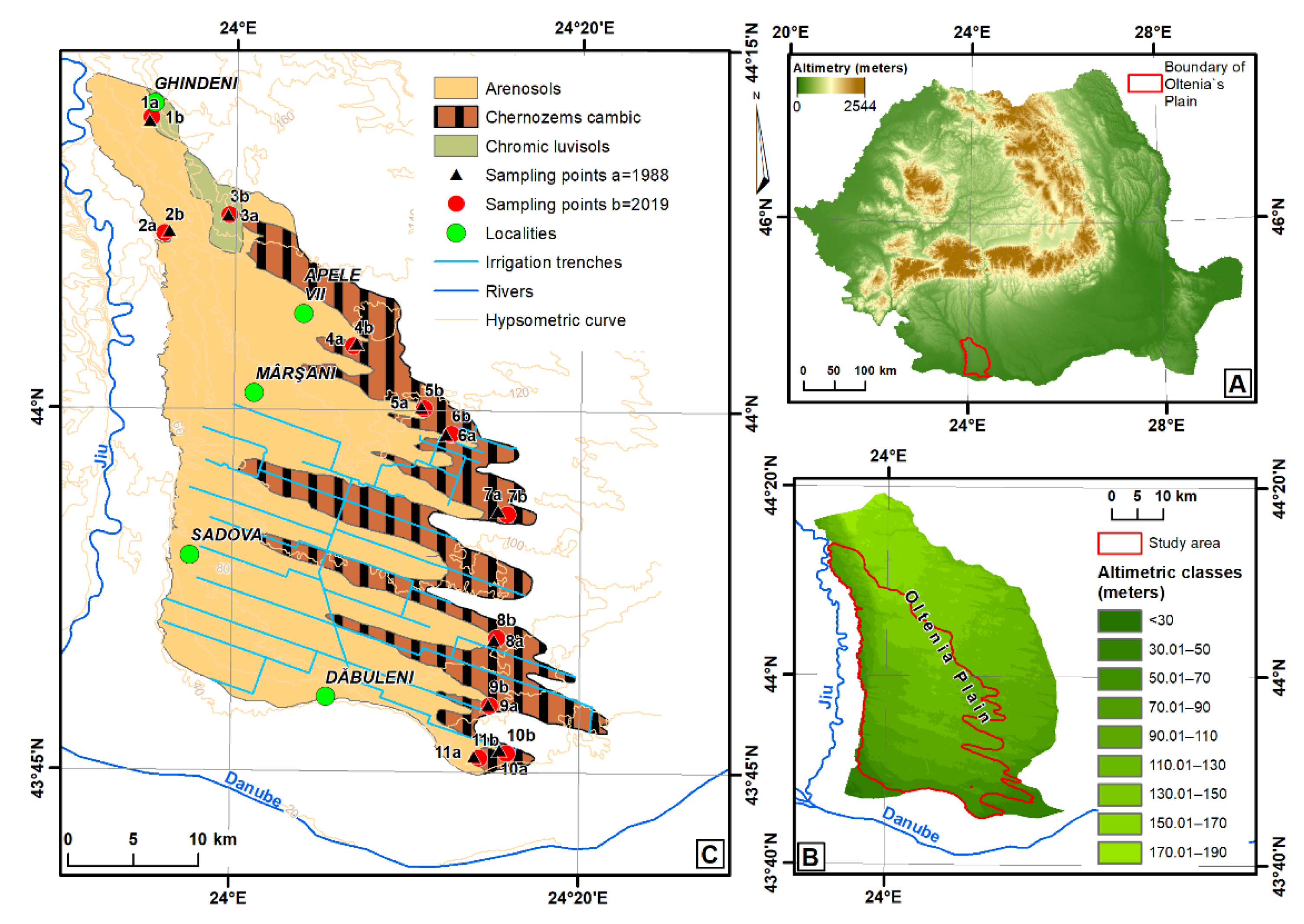
2. Study Area
3. Materials and Methods
3.1. Data Types
- a.
- Identification of the maximum uncovered sand areas during the year;
- b.
- Avoiding confusion between the light (yellow) colour of the sand and the straw resulting from grain harvesting;
- c.
- In autumn, plant residues are burnt and dark coloured surfaces can be confused with the soft horizon of Chernozems, while smoke influences the quality of the images;
- d.
- In winter, evapotranspiration is lower than in summer, therefore image quality will be less affected by the volume of vapour in the atmosphere. Winter evapotranspiration dynamics, analysed over a long period of time, was more stable compared to other seasons [40].
3.2. Data Processing
3.3. Normalized Sand Index (NSI)
- (a)
- Assessment of the accuracy of the NSI classification against the selected spectral indicator (NDSAI);
- (b)
- Assessment of the ability of traditional classification (TL) to map bare sand surfaces.
3.4. Accuracy of Traditional Classifications
4. Results and Discussion
5. Conclusions
Author Contributions
Funding
Data Availability Statement
Acknowledgments
Conflicts of Interest
References
- UN Climate Change Conference (COP26) at the SEC-Glasgow 2021. Available online: https://ukcop26.org (accessed on 10 April 2022).
- Bertran, P.; Bosq, M.; Borderie, Q.; Coussot, C.; Coutard, S.; Deschodt, L.; Franc, O.; Gardère, P.; Liard, M.; Wuscher, P. Revised Map of European Aeolian Deposits Derived from Soil Texture Data. Quat. Sci. Rev. 2021, 266, 107085. [Google Scholar] [CrossRef]
- Coteț, P. Oltenia Plain. Geomorphological Study (with Special Reference to the Quaternary); Scientific Publisher: Bucharest, Romania, 1957. [Google Scholar]
- Document of International Bank for Reconstruction and Development. Romania–Sadova–Corabia Agricultural Credit Project P-1555-RO (English); World Bank Group: Washington, DC, USA, 1975. [Google Scholar]
- Rusu, M.; Simion, G. Farm Structure Adjustments under the Irrigation Systems Rehabilitation in the Southern Plain of Romania: A First Step towards Sustainable Development. Carpathian J. Earth Environ. Sci. 2015, 10, 91–100. [Google Scholar]
- Pravalie, R. Aspects Regarding Spatial and Temporal Dynamic of Irrigated Agricultural Areas from Southern Oltenia in the Last Two Decades. Present Environ. Sustain. Dev. 2013, 7, 133–143. [Google Scholar]
- The Government of Romania. Low 18; The Government of Romania, Official Monitor: Bucharest, Romania, 1991.
- Vorovencii, I. Applying the Change Vector Analysis Technique to Assess the Desertification Risk in the South-West of Romania in the Period 1984–2011. Environ. Monit. Assess. 2017, 189, 524. [Google Scholar] [CrossRef]
- Nuta, S. Structural and functional characteristics of the forest curtains for the protection of the agricultural field in the south of Oltenia. Ann. For. Res. 2005, 48, 161–169. [Google Scholar]
- Achim, E.; Manea, G.; Vijulie, I.; Cocos, O.; Tirla, L. Ecological Reconstruction of the Plain Areas Prone to Climate Aridity through Forest Protection Belts. Case Study: Dabuleni Town, Oltenia Plain, Romania. Procedia Environ. Sci. 2012, 14, 154–163. [Google Scholar] [CrossRef][Green Version]
- Pravalie, R.; Sirodoev, I.; Peptenatu, D. Changes in the Forest Ecosystems in Areas Impacted by Aridization in South-Western Romania. J. Environ. Health Sci. Eng. 2014, 12, 2. [Google Scholar] [CrossRef]
- Rosca, F.C.; Harpa, G.V.; Croitoru, A.E.; Herbel, I.; Imbroane, A.M.; Burada, D.C. The Impact of Climatic and Non-Climatic Factors on Land Surface Temperature in Southwestern Romania. Theor. Appl. Clim. 2017, 130, 775–790. [Google Scholar] [CrossRef]
- Irimia, L.M.; Patriche, C.V.; LeRoux, R.; Quenol, H.; Tissot, C.; Sfica, L. Projections of climate suitability for wine production for the cotnari wine region (Romania). Present Environ. Sustain. Dev. 2019, 13, 5–18. [Google Scholar] [CrossRef]
- Dharumarajan, S.; Bishop, T.F.A.; Hegde, R.; Singh, S.K. Desertification Vulnerability Index-an Effective Approach to Assess Desertification Processes: A Case Study in Anantapur District, Andhra Pradesh, India. Land Degrad. Dev. 2018, 29, 150–161. [Google Scholar] [CrossRef]
- Fadhil Al-Quraishi, A.M. Land Degradation Detection Using Geo-Information Technology for Some Sites in Iraq. Al-Nahrain. J. Sci. 2009, 12, 94–108. [Google Scholar] [CrossRef]
- Fadhil Al-Quraishi, A.M. Sand Dunes Monitoring Using Remote Sensing and GIS Techniques for Some Sites in Iraq. In PIAGENG 2013: INTELLIGENT Information, Control, and Communication Technology for Agricultural Engineering; SPIE: Bellingham, WA, USA, 2013. [Google Scholar]
- Sahar, A.A.; Rasheed, M.J.; Uaid, D.A.A.-H.; Jasimm, A.A. Mapping Sandy Areas and Their Changes Using Remote Sensing. A Case Study at North-East Al-Muthanna Province, South of Iraq. Rev. Teledetec. 2021, 58, 39–52. [Google Scholar] [CrossRef]
- Wentzel, K. Determination of the Overall Soil Erosion Potential in the Nsikazi District (Mpumalanga Province, South Africa) Using Remote Sensing and GIS. Can. J. Remote Sens. 2002, 22, 322–327. [Google Scholar] [CrossRef]
- Zhao, H.; Chen, X.; Zhang, Z.; Zhou, Y. Exploring an Efficient Sandy Barren Index for Rapid Mapping of Sandy Barren Land from Landsat TM/OLI Images. Int. J. Appl. Earth Obs. Geoinf. 2019, 80, 38–46. [Google Scholar] [CrossRef]
- Afrasinei, G.M.; Melis, M.T.; Arras, C.; Pistis, M.; Buttau, C.; Ghiglieri, G. Spatiotemporal and Spectral Analysis of Sand Encroachment Dynamics in Southern Tunisia. Eur. J. Remote Sens. 2018, 51, 352–374. [Google Scholar] [CrossRef]
- Marzouki, A.; Dridri, A. Normalized Difference Enhanced Sand Index for desert sand dunes detection using Sentinel-2 and Landsat 8 OLI data, application to the north of Figuig, Morocco. J. Arid. Environ. 2022, 198, 104693. [Google Scholar] [CrossRef]
- Chen, S.; Ren, H.; Liu, R.; Tao, Y.; Zheng, Y.; Liu, H. Mapping Sandy Land Using the New Sand Differential Emissivity Index From Thermal Infrared Emissivity Data. IEEE Trans. Geosci. Remote Sens. 2021, 59, 5464. [Google Scholar] [CrossRef]
- Wang, X.; Song, J.; Xiao, Z.; Wang, J.; Hu, F. Desertification in the Mu Us Sandy Land in China: Response to climate change and human activity from 2000 to 2020. Geogr. Sustain. 2022, 3, 177. [Google Scholar] [CrossRef]
- Yang, Z.; Gao, X.; Lei, J.; Meng, X.; Zhou, N. Analysis of spatiotemporal changes and driving factors of desertification in the Africa Sahel. CATENA 2022, 213, 106213. [Google Scholar] [CrossRef]
- Guo, B.; Wei, C.; Yu, Y.; Liu, Y.; Li, J.; Meng, C.; Cai, Y. The dominant influencing factors of desertification changes in the source region of Yellow River: Climate change or human activity? Sci. Total Environ. 2022, 813, 152512. [Google Scholar] [CrossRef]
- Pan, X.; Zhu, X.; Yang, Y.; Cao, C.; Zhang, X.; Shan, L. Applicability of downscaling land surface temperature by using Normalized Difference Sand Index. Sci. Rep. 2018, 8, 9530. [Google Scholar] [CrossRef] [PubMed]
- Rasul, A.; Baltzer, H.; Faqe Ibrahim, G.R.; Hameed, H.M.; Wheeler, J.; Adamu, B.; Ibrahim, S.; Najmaddin, P.M. Applying Built-Up and Bare-Soil Indices from Landsat 8 to Cities in Dry Climates. Land 2018, 7, 81. [Google Scholar] [CrossRef]
- Simulescu, D. Geographical Study of Sandy Lands in the Romanati Plain. Ph.D. Thesis, Romanian Academy, Institute of Geography, Bucharest, Romania, 2019. [Google Scholar]
- Angearu, C.-V.; Ontel, I.; Boldeanu, G.; Mihailescu, D.; Nertan, A.; Craciunescu, V.; Catana, S.; Irimescu, A. Multi-Temporal Analysis and Trends of the Drought Based on MODIS Data in Agricultural Areas, Romania. Remote Sens. 2020, 12, 3940. [Google Scholar] [CrossRef]
- Bercea, I.; Dinucă, N.C. Considerations on Zoning and Micro-Zoning of the Dolj County Area for Potential Forest Vegetation in the Context of Anthropic Changes in Forest Lands and Climatic Changes. Ann. Univ. Craiova-Agric. Montanol. Cadastre Ser. 2018, 48, 18–34. [Google Scholar]
- Dudiak, N.; Pichura, V.; Potravka, L.; Stratichuk, N. Environmental and economic effects of water and deflation destruction of steppe soil in Ukraine. J. Water Land Dev. 2021, 50, 10. [Google Scholar] [CrossRef]
- WRB. World Reference Base for Soil Resources 2014, International Soil Classification System for Naming Soils and Creating Legend for Soil Map; FAO: Rome, Italy, 2014. [Google Scholar]
- Grigoraș, C.; Boengiu, S.; Vlăduț, A.; Grigoraș, E.N.; Avram, S. Romania’s Soils; Universitaria: Craiova, Romania, 2008; Volume 2. [Google Scholar]
- Ignat, P.; Gherghina, A.; Vrînceanu, A.; Anghel, A. Assesment of Degradation Processes and Limitative Factors Concerning the Arenosols from Dăbuleni–Romania. Geogr. Forum Stud. Res. Geogr. Environ. Prot. 2009, 8, 64–71. [Google Scholar]
- Stănilă, A.L.; Simota, C.C.; Dumitru, M. Contributions to the Knowledge of Sandy Soils from Oltenia Plain. Rev. Chim. 2020, 71, 192–200. [Google Scholar] [CrossRef]
- Landsat 8 Data Users Handbook|U.S. Geological Survey. Available online: https://www.usgs.gov/landsat-missions/landsat-8-data-users-handbook (accessed on 17 February 2022).
- Young, N.E.; Anderson, R.S.; Chignell, S.M.; Vorster, A.G.; Lawrence, R.; Evangelista, P.H. A Survival Guide to Landsat Preprocessing. Ecology 2017, 98, 920–932. [Google Scholar] [CrossRef]
- Guo, Q.; Fu, B.; Shi, P.; Cudahy, T.; Zhang, J.; Xu, H. Satellite Monitoring the Spatial-Temporal Dynamics of Desertification in Response to Climate Change and Human Activities across the Ordos Plateau, China. Remote Sens. 2017, 9, 525. [Google Scholar] [CrossRef]
- Salih, A.A.M.; Ganawa, E.T.; Elmahl, A.A. Spectral Mixture Analysis (SMA)-Change Vector Analysis (CVA) Methods for Monitoring-Mapping Land Degradation/Desertification in Arid-Semiarid Areas (Sudan), Using Landsat Imagery. Egypt. J. Remote Sens. Space Sci. 2017, 20, 22–29. [Google Scholar] [CrossRef]
- Pravalie, R. Analysis of temperature, precipitation and potential evapotranspiration trends in southern Oltenia in the context of climate change. Geogr. Tech. 2014, 9, 68. [Google Scholar]
- FAO. Guidelines for Soil Description, 4th ed.; Food and Agriculture Organization of the United Nations: Rome, Italy, 2006. [Google Scholar]
- Vos, C.; Axel, D.; Prietz, R.; Heidkamp, A.; Freibauer, A. Field-based soil-texture estimates could replace laboratory analysis. Geoderma 2016, 267, 215–219. [Google Scholar] [CrossRef]
- Munsell Color Co., Inc. Revised Washable Edition; GretagMacbeth: New Windsor, NY, USA, 2000. [Google Scholar]
- Gee, G.; Or, D. Particle-Size Analysis. In Methods of Soil Analysis; Physical Methods; Soil Science Society of America: Madison, WI, USA, 2002; pp. 255–293. [Google Scholar]
- Florea, N.; Munteanu, I. Romanian System of Soil Taxonomy, 2nd ed.; Sitech: Craiova, Romania, 2012. [Google Scholar]
- Chander, G.; Markham, B.L.; Helder, D.L. Summary of Current Radiometric Calibration Coefficients for Landsat MSS, TM, ETM+,-EO-1 ALI Sensors. Remote Sens. Environ. 2009, 113, 893–903. [Google Scholar] [CrossRef]
- Diek, S.; Fornallaz, F.; Schaepman, M.E.; Rogier De Jong. Barest Pixel Composite for Agricultural Areas Using Landsat Time Series. Remote Sens. 2017, 9, 1245. [Google Scholar] [CrossRef]
- Boettinger, J.L.; Ramsy, R.D.; Bodily, J.M.; Cole, N.J.; Kienast-Brown, S.; Nield, S.J.; Saunder, A.M.; Stum, A.K. Landsat Spectral Data for Digital Soil Mapping. In Digital Soil Mapping with Limited Data; Springer: Berlin/Heidelberg, Germany, 2008; pp. 193–202. [Google Scholar]
- Patel, N.; Kaushal, B. Improvement of User’s Accuracy through Classification of Principal Component Images and Stacked Temporal Images. Geo-Spat. Inf. Sci. 2010, 13, 243–248. [Google Scholar] [CrossRef]
- Lu, D.; Weng, Q. A Survey of Image Classification Methods and Techniques for Improving Classification Performance. Int. J. Remote Sens. 2007, 28, 823–870. [Google Scholar] [CrossRef]
- Bossard, M.; Feranec, J.; Otahel, J. CORINE Land Cover Technical Guide—Addendum 2000; Technical Report No 40; European Environmental Agency: Copenhagen, Denmark, 2000; p. 105. [Google Scholar]
- Dabboor, M.; Howell, S.; Shokr, M.; Yackel, J. The Jeffries–Matusita Distance for the Case of Complex Wishart Distribution as a Separability Criterion for Fully Polarimetric SAR Data. Int. J. Remote Sens. 2014, 35, 6859–6873. [Google Scholar] [CrossRef]
- Fongaro, C.; Demattê, J.; Rizzo, R.; Lucas Safanelli, J.; Mendes, W.; Dotto, A.; Vicente, L.; Franceschini, M.; Ustin, S. Improvement of Clay and Sand Quantification Based on a Novel Approach with a Focus on Multispectral Satellite Images. Remote Sens. 2018, 10, 1555. [Google Scholar] [CrossRef]
- Bindel, M.; Hese, S.; Berger, C.; Schmullius, C. Feature Selection from High Resolution Remote Sensing Data for Biotope Mapping. Int. Arch. Photogramm. Remote Sens. Spat. Inf. Sci. 2011, 38, 39–44. [Google Scholar] [CrossRef]
- Gong, P.; Wang, J.; Yu, L.; Zhao, Y.; Zhao, Y.; Liang, L.; Niu, Z.; Huang, X.; Fu, H.; Liu, S.; et al. Finer Resolution Observation and Monitoring of Global Land Cover: First Mapping Results with Landsat TM and ETM+ Data. Int. J. Remote Sens. 2013, 34, 2607–2654. [Google Scholar] [CrossRef]
- Wu, W.; Zucca, C.; Karam, F.; Liu, G. Enhancing the Performance of Regional Land Cover Mapping. Int. J. Appl. Earth Obs. Geoinf. 2016, 52, 422–432. [Google Scholar] [CrossRef]
- Curell, G.; Dowman, A. Essential Mathematics and Statistics for Science, 2nd ed.; Wiley-Blackwell: Hoboken, NJ, USA, 2009; 416p, ISBN 9780470694480. [Google Scholar]
- Reimann, R.C.; Filzmoster, P.; Garrett, R.G.; Dutter, R. Statistical Data Analysis Explained: Applied Environmental Statistics; John Wiley and Sons: Hoboken, NJ, USA, 2008; 343p. [Google Scholar] [CrossRef]
- Weiss, N.A. Introductory Statistics, 9th ed.; Pearson Education, Inc.: London, UK, 2012; 912p, ISBN 9780321691224. [Google Scholar]
- Zhang, J.; Liu, M.; Liu, X.; Luo, W.; Wu, L.; Zhu, L. Spectral analysis of seasonal rock and vegetation changes for detecting karst rocky desertification in southwest China. Int. J. Appl. Earth Obs. Geoinf. 2021, 100, 102337. [Google Scholar] [CrossRef]
- Zachentta, A.; Bitelli, G.; Karnieli, A. Monitoring desertification by remote sensing using the Tasselled Cap transform for long-term change detection. Nat. Hazards 2016, 83, 223. [Google Scholar] [CrossRef]
- Yu, H.; Liu, M.; Du, B.; Wang, Z.; Hu, L.; Zhang, B. Mapping Soil Salinity/Sodicity by using Landsat OLI Imagery and PLSR Algorithm over Semiarid West Jilin Province, China. Sensors 2018, 18, 1048. [Google Scholar] [CrossRef]
- Shao, G.; Tang, L.; Liao, J. Overselling Overall Map Accuracy Misinforms about Research Reliability. Landsc. Ecol. 2019, 34, 2487–2492. [Google Scholar] [CrossRef]
- Fung, T.; LeDrew, E. The Determination of Optimal Threshold Levels for Change Detection Using Various Accuracy Indices. Photogramm. Eng. Remote Sens. 1988, 54, 1449–1454. [Google Scholar]
- Kantakumar, L.N.; Neelamsetti, P. Multi-Temporal Land Use Classification Using Hybrid Approach. Egypt. J. Remote Sens. Space Sci. 2015, 18, 289–295. [Google Scholar] [CrossRef]
- Foody, G.M. Explaining the Unsuitability of the Kappa Coefficient in the Assessment and Comparison of the Accuracy of Thematic Maps Obtained by Image Classification. Remote Sens. Environ. 2020, 239, 111630. [Google Scholar] [CrossRef]
- Marinică, A.F.; Marinică, I.; Chimisliu, C. Climatic Variability in Southwestern Romania in the Context of Climate Changes during the Winter of 2018–2019. Stud. Commun. Nat. Sci. Olten. Mus. Craiova 2019, 35, 169–172. [Google Scholar]
- Tsoar, H. 11.21 Critical Environments: Sand Dunes and Climate Change. In Treatise on Geomorphology; Elsevier: Amsterdam, The Netherlands, 2013; pp. 414–427. [Google Scholar] [CrossRef]
- Marinica, I.; Chimisliu, C. Climatic Changes on Regional Plan in Oltenia and Their Effects on the Biosphere. Stud. Commun. Nat. Sci. Olten. Mus. Craiova 2008, 24, 221–229. [Google Scholar]
- Alexandru, D.; Mateescu, E.; Tudor, R.; Leonard, I. Analysis of Agroclimatic Resources in Romania in the Current and Foreseeable Climate Change—Concept and Methodology of Approaching. Agron. Ser. Sci. Res. 2019, 62, 221–229. [Google Scholar]
- Dumitraşcu, M.; Mocanu, I.; Mitrică, B.; Dragotă, C.; Grigorescu, I.; Dumitrică, C. The Assessment of Socio-Economic Vulnerability to Drought in Southern Romania (Oltenia Plain). Int. J. Disaster Risk Reduct. 2018, 27, 142–154. [Google Scholar] [CrossRef]
- Enescu, C.M. Sandy Soils from Oltenia and Carei Plains: A Problem or an Opportunity to Increase the Forest Fund in Romania? Sci. Pap. Ser. Manag. Econ. Eng. Agric. Rural Dev. 2019, 19, 203–206. [Google Scholar]
- Simulescu, D. The Impact of Human Activities on the Environment in the Romanați Plain (Romania), during the Postcommunist Era. Forum Geogr. 2018, 17, 123–134. [Google Scholar] [CrossRef]
- Petrișor, A.I.; Petrișor, L.E. 2006-2012 land cover and use changes in Romania—An overall assessment based on Corine data. Present Environ. Sustain. Dev. 2017, 11, 119–127. [Google Scholar] [CrossRef][Green Version]
- Ursu, A.; Stoleriu, C.C.; Ion, C.; Jitariu, V.; Enea, A. Romanian Natura 2000 Network: Evaluation of the Threats and Pressures through the Corine Land Cover Dataset. Remote Sens. 2020, 12, 2075. [Google Scholar] [CrossRef]
- Vladu, C.E. Reconversion/Restructuring of Vineyard Plantings in Oltenia in the Period 2007–2018 with the Access of European Funds. Ann. Univ. Craiova-Agric. Montanology Cadastre Ser. 2019, 49, 395–399. [Google Scholar]
- Andronache, I.; Fensholt, R.; Ahammer, H.; Ciobotaru, A.-M.; Pintilii, R.-D.; Peptenatu, D.; Drăghici, C.-C.; Diaconu, D.; Radulović, M.; Pulighe, G.; et al. Assessment of Textural Differentiations in Forest Resources in Romania Using Fractal Analysis. Forests 2017, 8, 54. [Google Scholar] [CrossRef]
- Lancaster, N. Dune Morphology and Dynamics. In Geomorphology of Desert Environments; Springer: Dordrecht, The Netherlands, 2009. [Google Scholar]
- Eger, P.; Almold, P.C.; Condron, L.M. Upbuilding Pedogenesis under Active Loess Deposition in a Super-Humid, Temperate Climate—Quantification of Deposition Rates, Soil Chemistry and Pedogenic Thresholds. Geoderma 2012, 189–190, 491–501. [Google Scholar] [CrossRef]


| Index | Bands Math | Feature Extraction, Sand Value/Climate | Satellite | References |
|---|---|---|---|---|
| Normalized Differential Sand Dune Index (NDSDI) | Sand, ˂0/dry | Landsat 5 TM, Landsat 7 ETM | [15] | |
| Normalized Differential Sand AreasIndex (NDSAI) | Sand, ˂0/dry or humid | Landsat 5 TM, Landsat 7 ETM, Landsat 8 OLI | [17] | |
| Normalized Difference Enhanced Sand Index (NDESI) | −2, +2/arid | Sentinel 2 and Landsat 8 OLI | [21] | |
| Sand differential emissivity index (SDEI) | 1 to 0.28/extremely arid | Aster | [22] |
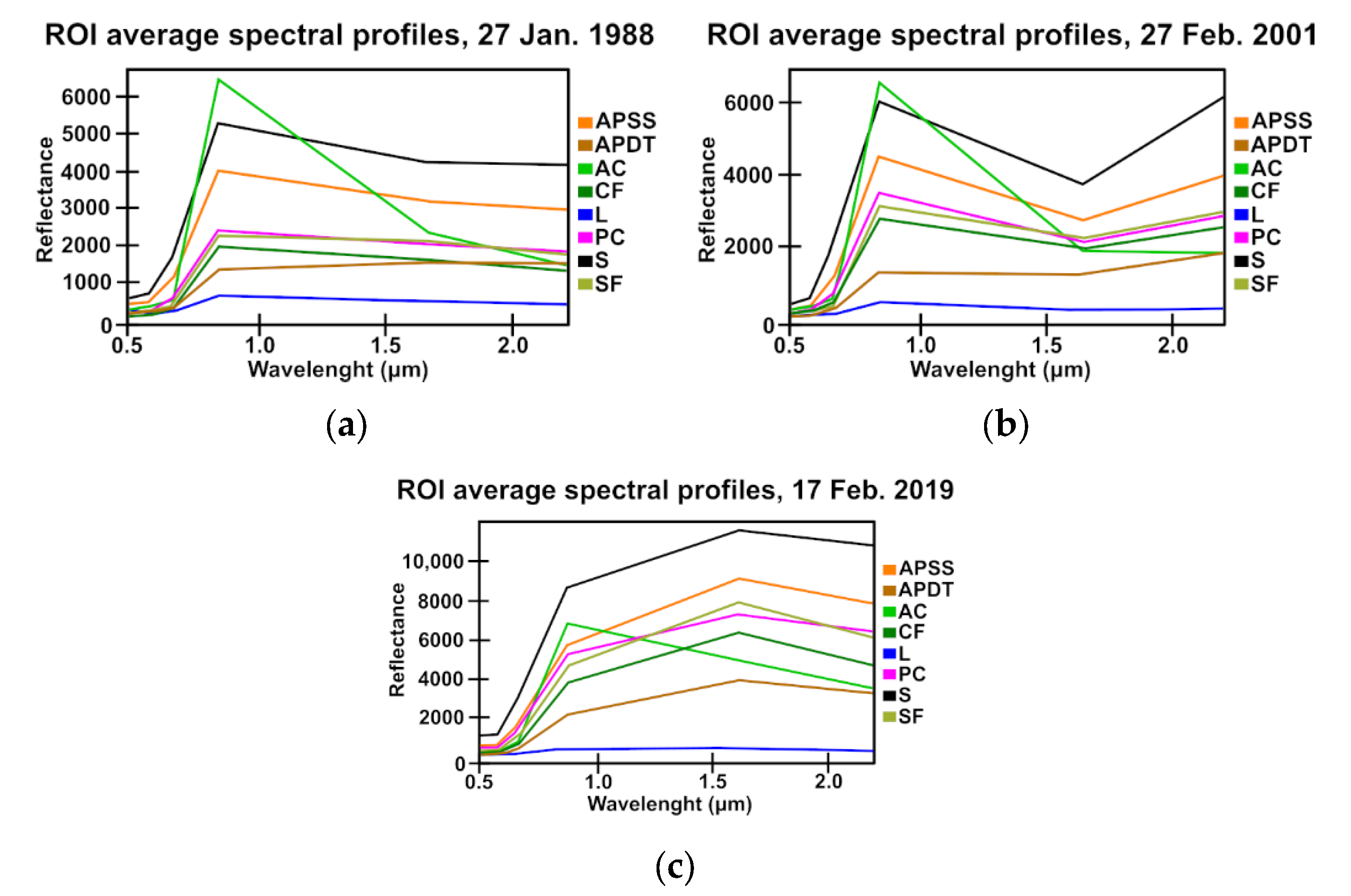
| Satellite | Row | Path | Date of Acquisition |
|---|---|---|---|
| Landsat 5 TM | 29 | 184 | 27 January 1988 |
| Landsat 7 ETM | 29 | 184 | 7 February 2001 |
| Landsat 8 OLI | 29 | 184 | 17 February 2019 |
| Index | Band Math | Feature Extraction, Sand Value/Climate | References |
|---|---|---|---|
| Normalized Differential Sand Dune Index (NDSDI) | Sand, ˂0/dry | [15] | |
| Normalized Differential Sand Areas Index (NDSAI) | Sand, ˂0/dry or humid | [17] |
| Land Use | Pixels Count for Each Land Use | ||
|---|---|---|---|
| 27 January 1988 | 7 February 2001 | 17 February 2019 | |
| Autumn crops (AC) | 7702 | 7730 | 4274 |
| Arable lands-pastures on sandy soils (APSS) | 3724 | 3213 | 2167 |
| Arable lands-pastures on different soil textures (APSDT) | 8651 | 7688 | 6104 |
| Permanent crops (PC) | 2995 | 1298 | 778 |
| Compact forests (CF) | 933 | 809 | 1619 |
| Scattered forests (SF) | 2123 | 4013 | 2140 |
| Sands (S) | 464 | 627 | 635 |
| Lakes (L) | 120 | 112 | 146 |
| Index | NSI 1988 | NDSAI 1988 | ||||||
|---|---|---|---|---|---|---|---|---|
| NSI (1) | NSI (2) | Total (User) | User Accuracy (%) | NDSAI (1) | NDSAI (2) | Total (User) | User Accuracy (%) | |
| Arenosol (1) | 42 | 8 | 50 | 84 | 44 | 9 | 53 | 83 |
| Other soil classes (2) | 3 | 5 | 8 | 62.5 | 1 | 4 | 5 | 80 |
| Total (Producer) | 45 | 13 | 58 | 0 | 45 | 13 | 58 | 0 |
| Producer accuracy (%) | 93.3 | 38.5 | 0 | 81.0 | 97.8 | 30.8 | 0 | 82.8 |
| Overall accuracy for arenosols (%) | 81.4 | 82 | ||||||
| NSI 2001 | NDSAI 2001 | |||||||
| Arenosol (1) | 44 | 8 | 52 | 84.6 | 43 | 9 | 52 | 82.7 |
| Other soil classes (2) | 1 | 5 | 6 | 83.3 | 2 | 4 | 6 | 66.7 |
| Total (Producer) | 45 | 13 | 58 | 0 | 45 | 13 | 58 | 0 |
| Producer accuracy (%) | 97.8 | 38.5 | 0 | 84.5 | 95.6 | 30.8 | 0 | 81 |
| Overall accuracy for arenosols (%) | 84.5 | 97 | ||||||
| NSI 2019 | NDSAI 2019 | |||||||
| Arenosol (1) | 43 | 8 | 51 | 84.3 | 44 | 10 | 54 | 81.5 |
| Other soil classes (2) | 2 | 5 | 7 | 74.4 | 1 | 3 | 4 | 75 |
| Total (Producer) | 45 | 13 | 58 | 0 | 45 | 13 | 58 | 0 |
| Producer accuracy (%) | 95.6 | 38.5 | 0 | 85.8 | 97.8 | 23.1 | 0 | 81 |
| Overall accuracy for arenosols (%) | 82.4 | 81 | ||||||
| MLK 1988 | MLK 2001 | MLK 2019 | ||||||||||
|---|---|---|---|---|---|---|---|---|---|---|---|---|
| Land Use | Prod. Acc. | User Acc. | Prod. Acc. | User Acc. | Pro. Acc. | User Acc. | Prod. Acc. | User Acc. | Prod. Acc. | User Acc. | Prod. Acc. | User Acc. |
| (%) | (%) | Pixels | Pixels | (%) | (%) | Pixels | Pixels | (%) | (%) | Pixels | Pixels | |
| AC | 98.87 | 95.64 | 263/266 | 263/275 | 93.24 | 92.34 | 193/207 | 193/209 | 100 | 99.38 | 641/641 | 641/645 |
| APSS | 95.68 | 86.46 | 332/347 | 332/384 | 92.27 | 85.42 | 334/362 | 334/391 | 62.99 | 93.27 | 291/462 | 291/312 |
| APSDT | 92.35 | 88.95 | 169/183 | 169/190 | 94.01 | 90.23 | 157/167 | 157/174 | 100 | 87.77 | 165/165 | 165/188 |
| PC | 79.82 | 77.39 | 178/223 | 178/230 | 81.72 | 80 | 228/279 | 228/285 | 62.07 | 31.03 | 36/58 | 36/116 |
| CF | 80.88 | 85.94 | 55/68 | 55/64 | 75.7 | 76.42 | 81/107 | 81/106 | 79.29 | 91.79 | 425/536 | 425/463 |
| SF | 58.08 | 80.83 | 97/167 | 97/120 | 61.54 | 79.28 | 88/143 | 88/111 | 85.96 | 57.83 | 251/292 | 251/434 |
| S | 66.67 | 94.74 | 18/27 | 18/19 | 52.17 | 92.31 | 12/23 | 12/13 | 92.65 | 94.19 | 227/245 | 227/241 |
| L | 75 | 100 | 3/4 | 3/3 | 0 | 0 | 0/1 | 0/0 | 100 | 100 | 56/56 | 56/56 |
| Soil Sample Code | Latitude | Longitude | Fine Sand a | Coarse Sand b | Sand | Land Use/Vegetation | Soils | Soil Colour c |
|---|---|---|---|---|---|---|---|---|
| 1a | 44°19′91″ | 23°91′59″ | 24.9 | 62.1 | 87 | Forest | Arenosols | 10YR8/8 |
| 1b | 44°20′16″ | 23°91′82″ | 71.2 | 22.1 | 93.3 | Arable | 10YR6/4 | |
| 2a | 44°12′31″ | 23°93′63″ | 49,8 | 36.2 | 93 | Herbaceous plants | Arenosols | 10YR6/4 |
| 2b | 44°12′16″ | 23°93′17″ | 12.6 | 87.1 | 86 | Herbaceous plants | 10YR7/6 | |
| 3a | 44°86′72″ | 23°59′34″ | 29.8 | 59.4 | 89.2 | Herbaceous plants (grassland) | Luvisols | 10YR6/3 |
| 3b | 44°83′93″ | 23°59′39″ | 49.5 | 41 | 90.5 | Herbaceous plants (grassland) | 10YR6/3 | |
| 4a | 44°24′64″ | 24°71′31″ | 19.2 | 70.5 | 89.7 | Arable | Chernozems | 10YR6/3 c |
| 4b | 44°24′10″ | 24°65′21″ | 13.8 | 79.6 | 93.4 | Arable | 10YR6/4 c | |
| 5a | 44°01′30″ | 24°10′49″ | 17.3 | 75.6 | 92.9 | Arable | Chernozems | 10YR6/3 c |
| 5b | 44°01′38″ | 24°10′49″ | 14.9 | 79 | 93.9 | Arable | 10YR5/3 | |
| 6a | 43°59′14″ | 24°12″ | 17.6 | 75.8 | 93.4 | Arable | Chernozems | 10YR5/3 |
| 6b | 43°98′41″ | 24°20′91″ | 8.3 | 87 | 95.3 | Arable | 10YR4/3 | |
| 7a | 43°55′49″ | 24°15′21″ | 14.8 | 77.7 | 92.5 | Vineyard | Chernozems | 10YR4/2 |
| 7b | 43°92′85″ | 24°26′41″ | 19.9 | 72.4 | 92.3 | Arable | 10YR5/3 | |
| 8a | 43°84′46″ | 24°25′56″ | 20.1 | 72.9 | 93.0 | Arable | Arenosols | 10YR4/3 |
| 8b | 43°84′49″ | 24°25′66″ | 19.8 | 71.9 | 91.7 | Arable | 10YR5/4 | |
| 9a | 43°79′66″ | 24°2′46″ | 52.4 | 33.4 | 85.8 | Herbaceous plants | Arenosols | 10YR5/2 |
| 9b | 43°79′64″ | 24°24′78″ | 25.4 | 62.9 | 88.3 | Arable | Cherozems | 10YR4/2 |
| 10a | 43°76′56″ | 24°25′77″ | 0.7 | 85 | 85.7 | Arable | Arenosols | 10YR4/4 |
| 10b | 43°76′34″ | 24°26′4″ | 57.6 | 38 | 95.6 | Arable | Cherozems | 10YR4/3 |
| 11a | 43°75′95″ | 24°23′46″ | 23.2 | 72.4 | 95.6 | Abandoned vineyard | Arenosols | 10YR4/4 |
| 11b | 43°75′88″ | 24°23′79″ | 25.1 | 62.4 | 87.5 | Abandoned vineyard | 10YR4/3 |
| Land Use | 27 January 1988 | 7 February 2001 | 17 February 2019 | |||
|---|---|---|---|---|---|---|
| MLK | MLK | MLK | ||||
| Pixel Count | % | Pixel Count | % | Pixel Count | % | |
| AC | 266,683 | 8.14 | 207,204 | 6.33 | 132,014 | 4.02 |
| APSS | 346,531 | 10.58 | 362,030 | 11.06 | 265,433 | 8.1 |
| APSDT | 184,225 | 5.62 | 168,077 | 5.13 | 265,382 | 8.1 |
| PC | 224,362 | 6.85 | 278,978 | 8.52 | 208,548 | 6.36 |
| CF | 68,577 | 2.09 | 106,872 | 3.26 | 141,542 | 4.32 |
| SF | 167,130 | 5.10 | 142,871 | 4.36 | 256,403 | 7.82 |
| S | 26,718 | 0.81 | 22,530 | 0.68 | 20,179 | 0.61 |
| L | 3920 | 0.11 | 1278 | 0.03 | 1214 | 0.03 |
Publisher’s Note: MDPI stays neutral with regard to jurisdictional claims in published maps and institutional affiliations. |
© 2022 by the authors. Licensee MDPI, Basel, Switzerland. This article is an open access article distributed under the terms and conditions of the Creative Commons Attribution (CC BY) license (https://creativecommons.org/licenses/by/4.0/).
Share and Cite
Secu, C.V.; Stoleriu, C.C.; Lesenciuc, C.D.; Ursu, A. Normalized Sand Index for Identification of Bare Sand Areas in Temperate Climates Using Landsat Images, Application to the South of Romania. Remote Sens. 2022, 14, 3802. https://doi.org/10.3390/rs14153802
Secu CV, Stoleriu CC, Lesenciuc CD, Ursu A. Normalized Sand Index for Identification of Bare Sand Areas in Temperate Climates Using Landsat Images, Application to the South of Romania. Remote Sensing. 2022; 14(15):3802. https://doi.org/10.3390/rs14153802
Chicago/Turabian StyleSecu, Cristian Vasilică, Cristian Constantin Stoleriu, Cristian Dan Lesenciuc, and Adrian Ursu. 2022. "Normalized Sand Index for Identification of Bare Sand Areas in Temperate Climates Using Landsat Images, Application to the South of Romania" Remote Sensing 14, no. 15: 3802. https://doi.org/10.3390/rs14153802
APA StyleSecu, C. V., Stoleriu, C. C., Lesenciuc, C. D., & Ursu, A. (2022). Normalized Sand Index for Identification of Bare Sand Areas in Temperate Climates Using Landsat Images, Application to the South of Romania. Remote Sensing, 14(15), 3802. https://doi.org/10.3390/rs14153802