MIMO Radar Sparse Recovery Imaging with Wideband Interference Prediction

Abstract

Multiple-input multiple-output (MIMO) radar three-dimensional (3D) imaging is widely applied in military and civil fields. However, MIMO is easily affected by wideband interference (WBI). To solve this problem, in this study, we propose a sparse recovery imaging method with WBI prediction based on the predictive recurrent neural network (PredRNN) and the tensor-based smooth L0 (TSL0) algorithm. Firstly, we extract the time-frequency (TF) feature of the historical measured WBI via the short-time Fourier transform (STFT) operation. In this way, we can use PredRNN to exploit the spatiotemporal correlation of the WBI in the TF domain to predict the TF feature of the WBI in the future. Then, we adaptively design the random sparse stepped frequency waveform by selecting non-overlapped frequencies with the WBI according to the predicted WBI TF feature. Finally, we apply the TSL0 algorithm to reconstruct the 3D high-resolution target image from the sparse signal cube. Simulation results show the high performance and robustness of the proposed imaging method in the presence of different WBIs.

1. Introduction

During the last decades, high-resolution radar images have been more and more widely used in both military and civil applications. Rather than two-dimensional (2D) images, three-dimensional (3D) radar images provide more details of the targets, which is crucial for target recognition and classification. For 3D target imaging, multiple-input multiple-output (MIMO) radar has been well developed in recent years [1,2,3,4,5] due to its single snap-shot imaging capacity. With the introduction of compressed sensing theory [6], studies have proposed many sparse recovery imaging methods for MIMO radar, bringing the advantages of lower sampling cost and higher resolution [7,8,9]. However, the complicated wideband interference (WBI) existing in the environment severely affects the received signal of MIMO radar, making the target imaging task difficult [10,11].

To improve radar imaging performance in the presence of WBI, WBI mitigation strategies have been extensively investigated, particularly in synthetic aperture radar (SAR) [10,11,12,13,14,15]. For example, by transforming the WBI problem into a narrowband interference (NBI) problem, Tao et al. proposed a WBI mitigation scheme for high-resolution airborne SAR [12]. Liu et al. exploited the sparsity of interference to develop a unified framework to mitigate WBI and recover the SAR signal at the same time [13]. In the time-frequency (TF) domain, Zhou et al. proposed the ways to detect and mitigate WBI based on variational Bayesian inference in [14] and instantaneous frequency estimation and regularized time-frequency filtering in [15]. These WBI mitigation techniques mainly attempt to eliminate the WBI signal from the radar received signal, which will inevitably damage the target signal to some extent, resulting in potential imaging performance loss.

Instead, another strategy is to design the transmitted waveform to minimize the impact of interference. For example, to increase target detection performance in the presence of interference, Wang et al. improved the signal-to-interference-ratio (SIR) of the transmitting signal by solving an optimization problem with the constraints of spectrum compatibility and constant modulus in [16]. Tierney and Mulgrew presented a scheme that combines interference spectrum estimation, adaptive waveform design, and waveform synthesis technique to minimize the interference in SAR [17]. Shi et al. tried to minimize the interference by optimizing the transmitting beam pattern by dividing the waveform matrix according to a power allocation strategy and by designing the sub-pulse waveforms for MIMO radar [18]. These waveform design strategies can obtain high performance for simple interferences, but they are less effective for the complicated ones (e.g., the interference is highly nonlinear or mixed by different interferences), necessitating the proposal of novel methods to address this issue.

In recent years, the rapid development and widespread application of the deep learning (DL) approach bring new solutions for interference suppression. For example, Fan et al. presented an interference mitigation algorithm based on the deep residual network for both NBI and WBI in [19], which can improve the radar performance with a low computational complexity. Tao et al. proposed a model-constrained DL approach based on the joint low-rank and sparse optimization framework, improving the efficiency of interference detection and mitigation [20]. In terms of waveform design in the presence of signal-dependent interference, Li et al. made a meaningful attempt by using the DL network to design the waveform for cognitive radar [21]. These DL based methods show promising prospects for interference suppression, while more efforts should be made to excavate the potentials of DL to solve more problems, e.g., MIMO radar target imaging problem in the presence of complicated WBIs.

To solve the above-mentioned problems of radar imaging in the WBI environment and inspired by the recent DL based studies, we propose a novel 3D high-resolution sparse recovery imaging method for MIMO radar with WBI prediction in this study. The contributions of this paper can be summarized as follows:

(1)

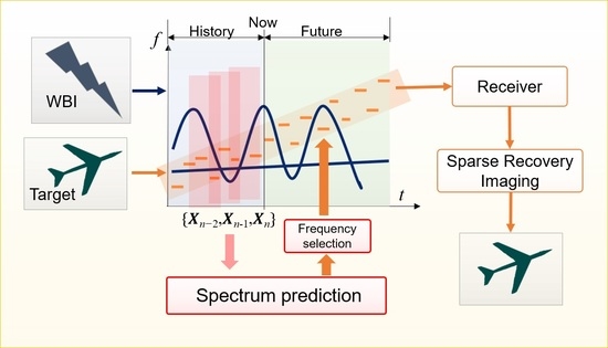
The DL based method for WBI prediction in the TF domain is proposed. We explore the spatiotemporal correlation of WBI in the TF domain and transform the WBI prediction problem into a spatiotemporal image sequence prediction problem. By using a sliding short-time Fourier transform (STFT) to process the measured WBI to generate a sequence of TF images, the TF images of the WBI in the future are predicted based on a trained DL network.

(2)

According to the predicted WBI, we adaptively design the random sparse stepped frequency (RSSF) waveform to make it orthogonal to the future WBI in the TF domain. By doing so, it brings two advantages as follows. Compared to the waveform design method based on historical WBI, the designed waveform with our method can adaptively avoid the WBI in the measurement. Compared to the WBI mitigation method, we can reserve the total information of target signal, since the designed waveform avoid the WBI to the maximum extent. Thus, we can improve the target imaging performance with the proposed method.

(3)

Furthermore, we apply the tensor-based smoothed L0 (TSL0) algorithm [22] to reconstruct the 3D high-resolution target image from the sparse received signal cube. With the WBI prediction and due to the advantages of sparse recovery, the proposed imaging method can obtain high effectiveness and robustness in different WBI environments, which are verified by various simulations.

The rest of this paper is organized as follows. Section 2 presents the signal model for MIMO radar 3D imaging and introduction of the imaging methods with WBI detection and removal (WDR) and simple waveform design (SWD), and finally presents the proposed imaging method with WBI prediction. Section 3 gives some simulation results to show the effectiveness and robustness of the proposed method. Section 4 discusses how to improve the performance of the proposed method with a view towards wider application. Finally, Section 5 concludes this paper.

2. Materials and Methods

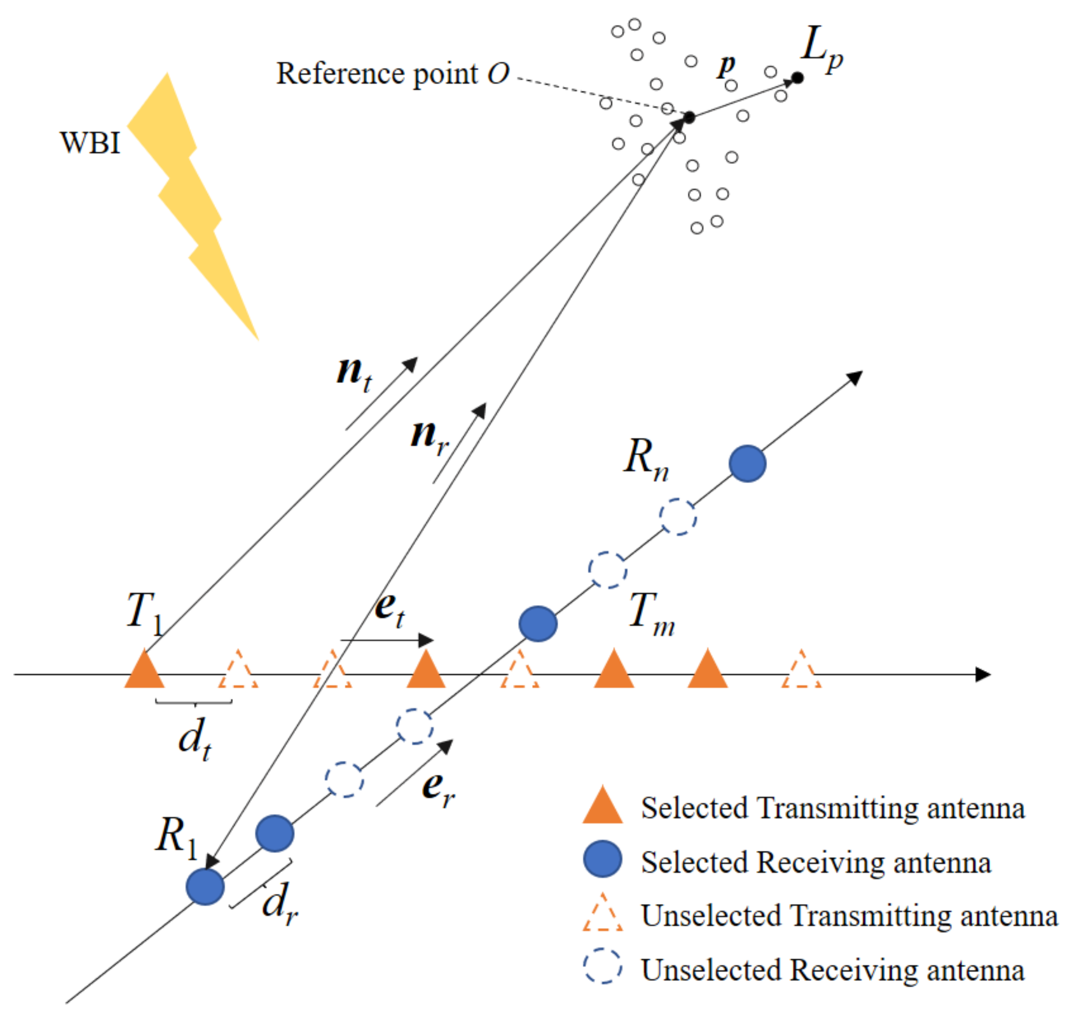
2.1. Signal Model

As shown in Figure 1, we consider a 2D cross MIMO radar consisting of orthogonal uniform linear transmitting and receiving arrays, formed by M transmitting antennas and N receiving antennas. The transmitting and receiving antenna spacings are denoted by d_t and d_r, respectively. The unitary direction vectors of the transmitting and receiving arrays are denoted by e_t and e_r, respectively. A sparse MIMO array is generated with M_u (0 < M_u < M) transmitting antennas and N_u (0 < N_u < N) receiving antennas, randomly selected from the full transceiving arrays. A target viewed as P scattering points is in the imaging area with L_p denoting the p-th scattering point ($p=1,2,\dots ,P$) and O denoting the reference point. The direction vector from O to L_p is denoted as p = (x_p, y_p, z_p) with x_p, y_p, and z_p as the 3D positions of the p-th scattering point relative to the reference point.

We adopt the RSSF waveform that is commonly employed in radar imaging for wide bandwidth synthesis in this study [23]. For RSSF, the q-th sub-pulse signal can be expressed as

$$s^q(t)=rect[(t-(q-1)T_r)/T_r]e^{j2\pi f_{q}t}$$

(1)

where $q=1,2,\dots ,Q_u$, Q_u < Q is the number of sub-pulses, $t\in [0,T_s]$, T_s = Q_uT_r is the total signal duration, T_r is the duration of each sub-pulse, $rect[\cdot ]$ is the rectangle function, $f_q\in \mathcal{F}$ is the q-th frequency, which is randomly selected from a given frequency sequence $\mathcal{F}=[f_1,f_2,\dots ,f_Q]$. In $\mathcal{F}$, $f_i=f_1+(i-1)\Delta f$, where $i=1,2,\dots ,Q$ and $\Delta f$ denotes the frequency step.

To ensure the orthogonality of different transmitting signals, we modulate the RSSF signals of different transmitting antennas with the orthogonal phase codes. Thus, the q-th sub-pulse signal of the m-th ($m=1,2,\dots ,M_u$) transmitting antenna can be expressed as

$$s_T^{m,q}(t)=s^q(t)e^{j{\phi }^m(t)}$$

(2)

where ${\phi }^m(t)$ is the modulation phase code of the m-th transmitting antenna.

Backscattering from the target and considering the WBI signal in the environment, the q-th sub-pulse signal received by the n-th ($n=1,2,\dots ,N_u$) receiving antenna can be expressed as

$$s_R^{n,q}(t)={\displaystyle \sum _{p=1}^P{\displaystyle \sum _{m=1}^{M_u}{\varsigma }_p{s}_T^{m,q}(t-{\tau }_{m,n,p})}}+I(t)$$

(3)

where ${\tau }_{m,n,p}$ and ${\varsigma }_p$ denote the delay and scattering coefficient of the p-th scattering point, respectively, $I(t)$ is the received WBI that is assumed to be independent from the transceiving channels. According to the geometric relationship shown in Figure 1, ${\tau }_{m,n,p}$ can be derived as ${\tau }_{m,n,p}=(\left|T_m{L}_p\right|+\left|L_p{R}_n\right|)/c$, where $\left|T_m{L}_p\right|$ is the distance from the m-th transmitting antenna to the p-th scattering point, $\left|L_p{R}_n\right|$ is the distance from the n-th receiving antenna to the p-th scattering point, and c is the speed of light.

By mixing with a reference signal, we can down-convert the received signal $s_R^{n,q}(t)$ to

$$s_D^{m,n,q}(t)=s_R^{n,q}(t)\cdot e^{-j2\pi f_q(t-{\tau }_{m,n,O})}$$

(4)

where ${\tau }_{m,n,O}=(|T_{m}O|+|O{R}_n|)/c$ is the delay of the reference point corresponding to m-th transmitting antenna and the n-th receiving antenna.

Via digital sampling, we can get $s^{m,n,q}(k_s)$ from $s_D^{m,n,q}(t)$, where $k_s=f_{s}t=1,2,\dots ,K_s$ is the k_s-th sampling index and f_s is the sampling rate. Then, we can use the matched filtering (MF) based method to realize the waveform separation, giving

$$s_M^{m,n,q}({k^{\prime }}_s)={\displaystyle \sum _{k_s=1}^{K_s}{s}^{m,n,q}(k_s)}\cdot e^{-j{\phi }^m(k_s-{k^{\prime }}_s)}/K_s$$

(5)

As the bandwidth of each sub-pulse is small, all the scattering points of the target will locate at the same range cell in (5). Hence, by selecting the peak of (5), we can get a 3D signal cube $S\in {ℂ}^{M_u\times N_u\times Q_u}$ for target imaging, whose m-n-q-th element is given by

$$S(m,n,q)=\left\{\begin{array}{cc}{S}_0(m,n,q)+\mathcal{I}(m,n,q),\hfill & \hspace{1em}q=q_I^C\\ S_0(m,n,q),\hfill & \hspace{1em}q\ne q_I^C\end{array}\right.$$

(6)

where $S_0$ is the target signal cube and $\mathcal{I}$ is the WBI component. As the WBI frequency is varying along with time, the target signal cube corresponding to the sub-pulse indexed by $q\ne q_I^C\in {\Gamma }_I^C$ will not be interfered by the WBI, while ${\Gamma }_I^C$ denotes the index set of the interfered sub-pulses.

According to [4,5], the m-n-q-th element of the target signal cube $S_0$ can be approximated as

$$S_0(m,n,q)={\displaystyle \sum _{p=1}^P{\varsigma }_p{e}^{-j2\pi {\alpha }_p{x}_m/d_t}{e}^{-j2\pi {\beta }_p{y}_n/d_r}{e}^{-j2\pi {\chi }_p{f}_q/\Delta f}}$$

(7)

where $x_m$ and $y_n$ denote the positions of the m-th transmitting antenna and the n-th receiving antenna, ${\alpha }_p$, ${\beta }_p$, and ${\chi }_p$ denote the parameters of the p-th scattering point, which have the following relationships with the 3D positions of the p-th scattering point

$$\left\{\begin{array}{l}{\alpha }_p=-{\mathit{e}}_t^T\mathit{p}{d}_t/({\lambda }_c{r}_T),\hspace{1em}{\beta }_p=-{\mathit{e}}_r^T\mathit{p}{d}_r/({\lambda }_c{r}_R)\\ {\chi }_p={({\mathit{n}}_t+{\mathit{n}}_r)}^T\mathit{p}+[1/(2r_T)+1/(2r_R)]{\mathit{p}}^T\mathit{p}\Delta f/c\end{array}\right.$$

(8)

where ${\lambda }_c=c/f_c$ is the wavelength, $f_c$ is the carrier frequency, $r_T=\left|T_{1}O\right|$ is the distance from the reference point to the first transmitting antenna, $r_R=\left|O{R}_1\right|$ is the distance from the reference point to the first receiving antenna, while ${\mathit{n}}_t$ and ${\mathit{n}}_r$ are the unitary direction vectors of $\overrightarrow{T_{1}O}$ and $\overrightarrow{R_{1}O}$, as shown in Figure 1.

If there is no WBI or the WBI component $\mathcal{I}$ in the signal cube $\mathcal{S}$ can be eliminated, according to (7), we can express the signal cube $\mathcal{S}$ as

$$\mathcal{S}=\mathcal{X}{\times }_1{\mathit{F}}_{un}^1{\times }_2{\mathit{F}}_{un}^2{\times }_3{\mathit{F}}_{un}^3$$

(9)

where $\mathcal{X}\in {ℝ}^{M_0\times N_0\times Q_0}$ denotes the 3D image of the target, M₀, N₀, and Q₀ are the imaging grid numbers in the directions discretized to estimate the target parameters ${\alpha }_p$, ${\beta }_p$, and ${\chi }_p$ for $p=1,2,\dots ,P$. ×κ denotes the mode-κ tensor by matrix product. In (9), ${\mathit{F}}_{un}^1$, ${\mathit{F}}_{un}^2$, and ${\mathit{F}}_{un}^3$ are the Fourier matrices corresponding to the selected antennas and sub-pulses, given by

$$\left\{\begin{array}{l}{\mathit{F}}_{un}^1=e^{-j2\pi {[x_1,x_2,\dots ,x_{Mu}]}^T{\mathit{\alpha }}_0/d_t}\in C^{M_u\times M_0}, {\mathit{\alpha }}_0=[-1/2,-1/2+1/M_0,\dots ,1/2-1/M_0]\\ {\mathit{F}}_{un}^2=e^{-j2\pi {[y_1,y_2,\dots ,y_{Nu}]}^T{\mathit{\beta }}_0/d_r}\in C^{N_u\times N_0}, {\mathit{\beta }}_0=[-1/2,-1/2+1/N_0,\dots ,1/2-1/N_0]\\ {\mathit{F}}_{un}^3=e^{-j2\pi {[f_1,f_2,\dots ,f_{Qu}]}^T{\mathit{\chi }}_0/\Delta f}\in C^{Q_u\times Q_0}, {\mathit{\chi }}_0=[-1/2,-1/2+1/Q_0,\dots ,1/2-1/Q_0]\end{array}\right.$$

(10)

By exploiting the sparsity of the target in the imaging area, we can solve the following problem for 3D high-resolution target imaging

$$min{∥\mathcal{X}∥}_0\mathrm{s}.\mathrm{t}.∥\mathcal{S}-\mathcal{X}{\times }_1{\mathit{F}}_{un}^1{\times }_2{\mathit{F}}_{un}^2{\times }_3{\mathit{F}}_{un}^3∥\underline{{}_{\mathrm{F}}}\le \epsilon$$

(11)

where ${‖\cdot ‖}_0$ and $‖\cdot ‖\underset{¯}{{}_{\mathrm{F}}}$ denote the number of nonzero elements and the Frobenius norm of a tensor, $\epsilon$ denotes the noise level.

Directly solving (11) is difficult. Hence, we transform it to the following problem

$$\min \underset{\partial \to 0}{\lim }{G}_{\partial }(\mathcal{X}) \mathrm{s}.\mathrm{t}. ‖\mathcal{S}-\mathcal{X}{\times }_1{\mathit{F}}_{un}^1{\times }_2{\mathit{F}}_{un}^2{\times }_3{\mathit{F}}_{un}^3‖\underset{¯}{{}_{\mathrm{F}}}\le \epsilon$$

(12)

where $\partial$ is an auxiliary variable that is close to zero and

$$G_{\partial }(\mathcal{X})=M_0{N}_0{Q}_0-{\displaystyle \sum _{m_0=1}^{M_0}{\displaystyle \sum _{n_0=1}^{N_0}{\displaystyle \sum _{q_0=1}^{Q_0}\exp (-{\left|{\mathcal{X}}_{m_0,n_0,q_0}\right|}^2/2{\partial }^2)}}}$$

(13)

with ${\mathcal{X}}_{m_0,n_0,q_0}$ as the m₀-n₀-q₀-th element of $\mathcal{X}$.

Equation (12) can be solved effectively by the TSL0 algorithm [22]. After obtaining $\mathcal{X}$, the target parameters {α, β, χ} = {[α₁,α₂,…,α_P], [β₁,β₂,…,β_P], [χ₁,χ₂,…,χ_P]} can be extracted. Then, we can get the target positions {x, y, z} = {[x₁,x₂,…,x_P], [y₁,y₂,…,y_P], [z₁,z₂,…,z_P]} based on (8).

Although the sparse recovery imaging method based on (12) has high performance, the WBI component $\mathcal{I}$ in the signal cube $\mathcal{S}$ has a highly negative impact on the imaging result. The key to solve this problem is to get the signal cube for target imaging without the WBI influence. Many meaningful attempts are made, which are mainly from two perspectives. Most studies focus on mitigating the WBI component from the signal cube by some post-processing methods [12,13,14,15] while others are interested in minimizing the WBI component by some preprocessing methods [16,17,18].

2.2. Conventional Imaging Methods

2.2.1. Imaging Method with WDR

To mitigate the WBI component from the signal cube for target imaging, many methods can be used, e.g., those in [12,13,14,15]. In this study, we consider a simple way (i.e., WDR) to do so, i.e., detecting and removing the interfered signal components including target signal and WBI directly from the signal cube, expressed as

$$S(m,n,q)=\left\{\begin{array}{cc}0,\hfill & q=q_I^C\\ S_0(m,n,q),\hfill & q\ne q_I^C\end{array}\right.$$

(14)

Since the WBI is always much stronger than the target signal, the interfered sub-pulses can be easily detected via some existing approaches, such as the constant false alarm rate (CFAR) detection technique. Then, the set ${\Gamma }_I^C$ can be obtained and the interfered signal components can be set to 0. Finally, by neglecting the zero elements, the signal cube shown in (14) can be used for target imaging via the TSL0 algorithm.

It should be noted that, for existing methods used to mitigate the WBI component, the target signal in the interfered sub-pulses will be damaged to some extent, i.e., some of the target information will be removed, as the WBI component and the target signal cannot be exactly estimated without any error. Compared to these methods, the WDR method may have worse performance as it removes all the target information in the interfered sub-pulses. However, the WDR method can be easily realized and can perform well under the situations where the WBI does not occupy a large space in the TF domain, i.e., fewer sub-pulses are interfered by the WBI.

2.2.2. Imaging Method with SWD

To minimize the WBI component in the signal cube for target imaging, many preprocessing methods pay attention to design waveform to reduce the WBI by increasing the SIR or to directly avoid receiving the WBI. In this study, we also consider a simple way (i.e., SWD) to do so, i.e., designing a transmitting waveform that is orthogonal to the WBI in the TF domain according to the historical measured WBI.

For the measured WBI, we employ the STFT to extract its TF feature, expressed as

$$\mathit{X}(t,f)=|{\displaystyle {\int }_{-\infty }^{+\infty }x(\tau )h(\tau -t)e^{-j2\pi f\tau }d\tau }|$$

(15)

where h(t) denotes the windowing function.

For SWD, given T > T_s as the total duration of the measured WBI, the WBI TF feature in the duration of $t\in [T-T_s,T]$ is used for the transmitting waveform design in the duration of $t\in [T,T+T_s]$. Specific to the RSSF waveform, the frequency of the q-th sub-pulse is designed as

$$f_q=\mathcal{F}(i_q\in \mathcal{L}\backslash {\mathcal{U}}_q^{HMW})$$

(16)

where $i_q$ denotes the index of the q-th selected frequency and $\mathcal{L}=[1,2,\dots ,Q]$. The superscript HMW in (16) denotes the first letters of historical measured WBI and ${\mathcal{U}}_q^{HMW}$ denotes the non-selectable frequency index set for the q-th sub-pulse, expressed as

$${\mathcal{U}}_q^H\leftarrow \left\{\begin{array}{cc}{I}_1^{HMW},\hfill & q=1\\ \{i_1,\dots ,i_{q-1}\}\cup I_q^{HMW},\hfill & q\ge 2\end{array}\right.$$

(17)

where $I_q^{HMW}$ denotes the frequency index set for the q-th sub-pulse of the measured WBI in the duration of $t\in [T-T_s+(q-1)T_r,T-T_s+q{T}_r]$, which is obtained from $\mathit{X}(t,f)$.

By transceiving the designed RSSF waveform, the WBI component in the signal cube can be reduced or avoided. Hence, without WBI mitigation, we can directly apply the TSL0 algorithm to process the signal cube given in (6) to obtain the 3D high-resolution target image. It should be noted that, with some additional processing steps, e.g., WBI parameter estimation, many existing methods also use the historical measured WBI as the reference for waveform design. Compared to these methods, the performance of the SWD method may degrade when the future WBI TF feature is quite different from its historical one. However, the SWD method has the advantage of simplicity, and it can obtain reasonable results when the WBI is relatively stationary.

2.3. Proposed Imaging Method

As mentioned above, the WBI mitigation methods have the problem of damaging the target signal. In general, if the transmitting waveform can be designed to be completely orthogonal to the WBI in the TF domain, there is no need to do WBI mitigation and then the target signal will not be damaged. However, because of either the high computational cost or the need of prior WBI model for parameter estimation, existing waveform design methods are less effective for complicated WBIs. To solve these problems, we propose a novel imaging method with WBI prediction to improve the MIMO radar imaging performance in the environment with complicated WBIs.

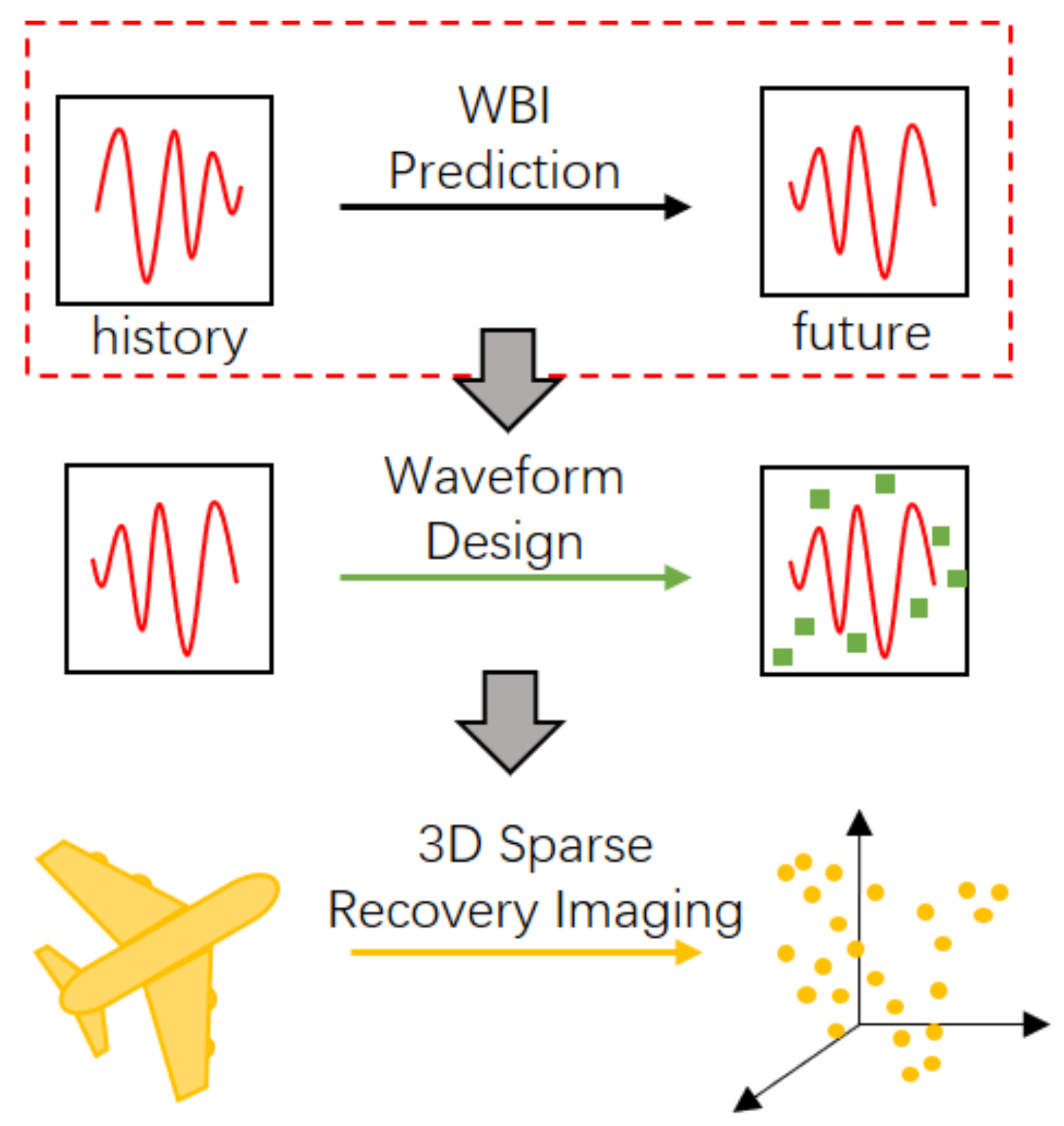
2.3.1. Framework of Our Method

The core of the proposed imaging method is WBI prediction and its other processing steps are similar with the SWD method. It is known that, if the future TF feature of the WBI can be obtained beforehand, the radar transmitting waveform can be adaptively designed to reduce or even avoid the influences of WBI on the received signal. Recently, for spatiotemporal image sequence prediction problems, e.g., automatic driving, robot motion planning, and precipitation forecasting, the deep predictive networks, such as ConvLSTM (Convolutional Long Short-Term Memory) [24] and PredRNN [25], have been well developed. For WBI prediction, whose TF feature can also be exploited with a high spatiotemporal correlation, it is suitable to apply the deep predictive network.

Based on the idea of WBI prediction, Figure 2 shows the framework of the proposed sparse recovery imaging method for MIMO radar.

The first and most important step of the proposed imaging method, which is circled by the red dotted rectangle in Figure 2, is to predict the future WBI according to the historical measured WBI. We will introduce this step in detail in the following subsection. The second step of the proposed imaging method is to design the waveform based on (16) with ${\mathcal{U}}_q^{PW}$ instead of ${\mathcal{U}}_q^{HMW}$, which is obtained according to the predicted TF feature of the WBI, where the superscript PW denotes the first letters of predicted WBI. It should be noted that, in such a case, $I_q^{HMW}$ in (17) should be replaced with $I_q^{PW}$, which is the frequency index set of the q-th sub-pulse interfered by the predicted WBI in the duration of $t\in [T+(q-1)T_r,T+q{T}_r]$. As the designed waveform is orthogonal to WBI in the TF domain, the sparse signal cube in (6) is simply $\mathcal{S}(m,n,q)={\mathcal{S}}_0(m,n,q)$ with ${\Gamma }_I^C=\varnothing$. Thus, the last step of the proposed method is to directly apply the TSL0 algorithm to solve (12) to get the 3D high-resolution target image.

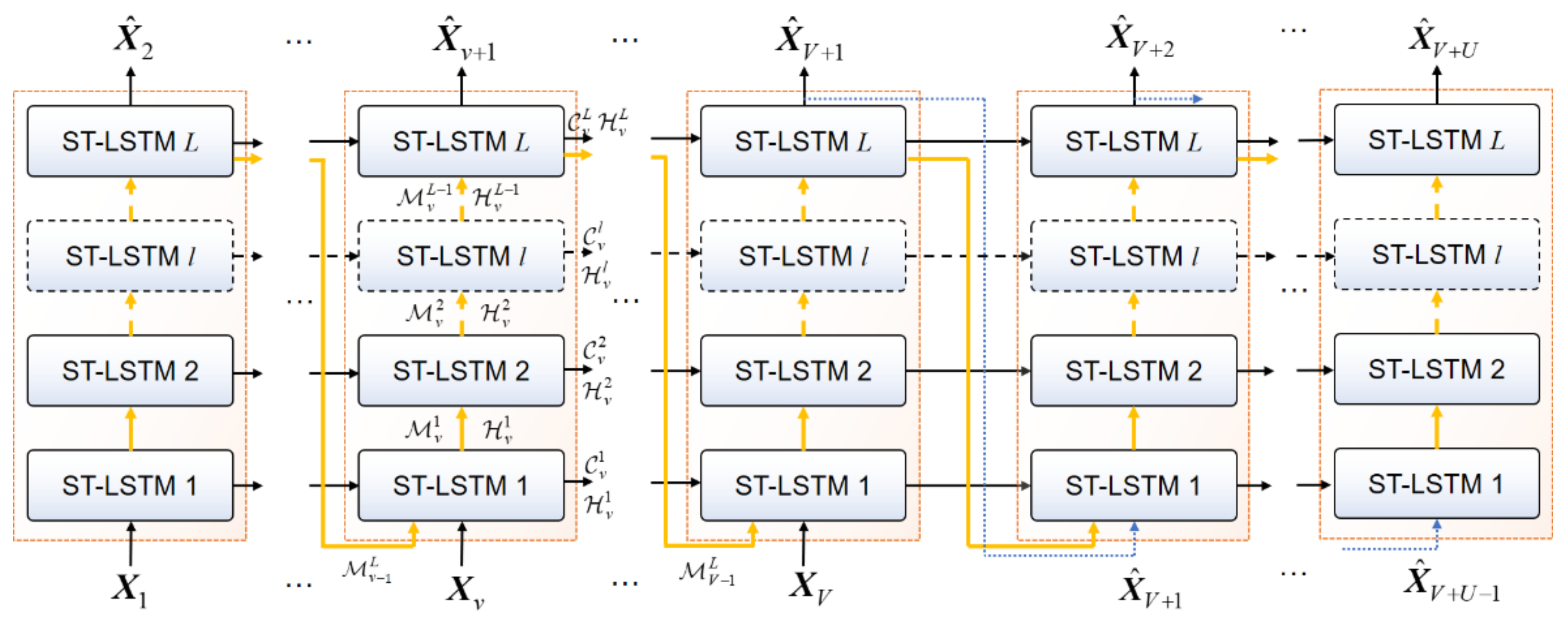
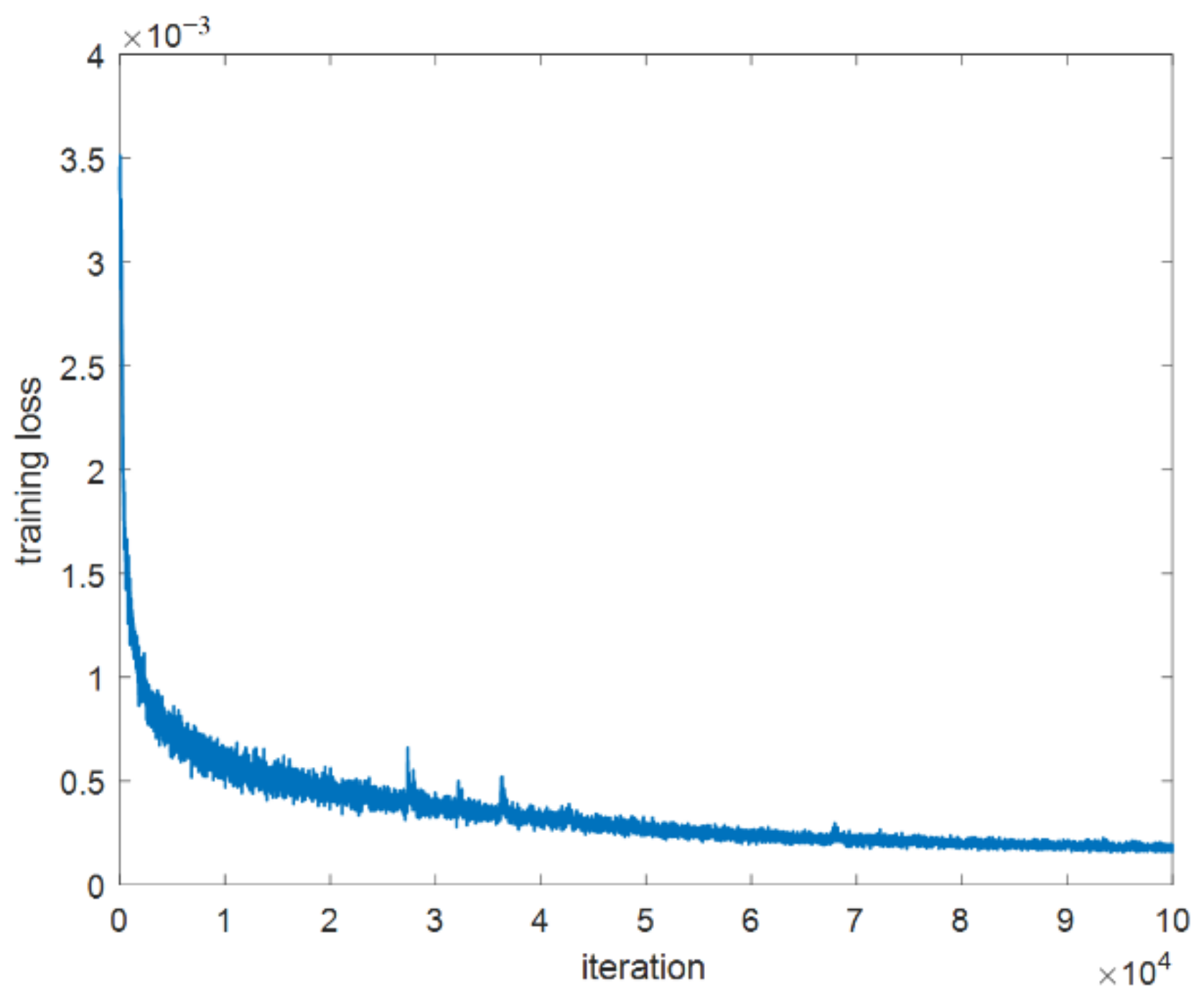
2.3.2. WBI Prediction via PredRNN

Introduction of PredRNN

Considering its high performance in spatiotemporal image sequence prediction, we use PredRNN in this study to predict the WBI. Figure 3 shows the structure of an L-layer PredRNN, whose basic module is the spatiotemporal LSTM (ST-LSTM), which combines the long-time information with the short-time information and takes the continuity of the same layer in time and the hierarchy of different layers in space into account.

As shown in Figure 3, the input of PredRNN is $\underset{¯}{{\mathit{X}}_I}=〈{\mathit{X}}_1,{\mathit{X}}_2,{\mathit{X}}_3,\dots ,{\mathit{X}}_V〉$ and the output of PredRNN is $\underset{¯}{{\widehat{\mathit{X}}}_O}=〈{\widehat{\mathit{X}}}_2,{\widehat{\mathit{X}}}_3,\dots ,{\widehat{\mathit{X}}}_V,{\widehat{\mathit{X}}}_{V+1},{\widehat{\mathit{X}}}_{V+2},\dots ,{\widehat{\mathit{X}}}_{V+U}〉$, where V denotes the number of input images and U denotes the number of output images. Hence, the task of PredRNN can be expressed as $\underset{¯}{{\mathit{X}}_I}\mapsto \underset{¯}{{\widehat{\mathit{X}}}_O}$. We note that, as indicated by the blue dotted curves in Figure 3, the outputs $〈{\widehat{\mathit{X}}}_{V+1},{\widehat{\mathit{X}}}_{V+2},\dots ,{\widehat{\mathit{X}}}_{V+U-1}〉$ are also used as the inputs of PredRNN to predict the sequences $〈{\widehat{\mathit{X}}}_{V+2},{\widehat{\mathit{X}}}_{V+3},\dots ,{\widehat{\mathit{X}}}_{V+U}〉$.

According to [25], the overall process of PredRNN used to predict the image ${\widehat{\mathit{X}}}_{v+1}$ ($v=1,2,\dots ,V+U-1$) can be expressed as

$$\left\{\begin{array}{c}\left\{{\mathcal{H}}_v^1,{\mathcal{C}}_v^1,{\mathcal{M}}_v^1\right\}=\mathrm{ST}-\mathrm{LST}{\mathrm{M}}_1({\mathit{X}}_v,{\mathcal{M}}_{v-1}^L,{\mathcal{H}}_{v-1}^1,{\mathcal{C}}_{v-1}^1)\hfill \\ \left\{{\mathcal{H}}_v^l,{\mathcal{C}}_v^l,{\mathcal{M}}_v^l\right\}=\mathrm{ST}-\mathrm{LST}{\mathrm{M}}_l({\mathcal{H}}_v^{l-1},{\mathcal{M}}_v^{l-1},{\mathcal{H}}_{v-1}^l,{\mathcal{C}}_{v-1}^l)\hfill \\ {\widehat{\mathit{X}}}_{v+1}={\mathcal{W}}_v*{\mathcal{H}}_v^{L}l=2,\dots ,L\hfill \end{array}\right.$$

(18)

where $\ast$ denotes convolution operation, ${\mathcal{H}}_v^l$, ${\mathcal{C}}_v^l$, and ${\mathcal{M}}_v^l$ denote the hidden state, the temporal memory, and the spatiotemporal memory for the v-th input image in the l-th ST-LSTM layer ($l=1,2,\dots ,L$).

For the l-th ST-LSTM, assuming its input is generalized as $(A_v^l,B_v^l,E_v^l,F_v^l)$, its output $({\mathcal{H}}_v^l,{\mathcal{C}}_v^l,{\mathcal{M}}_v^l)$ can be obtained by

$$\left\{\begin{array}{l}{g}_v^l=\tanh ({\mathcal{W}}_{ag}^l\ast A_v^l+{\mathcal{W}}_{eg}^l\ast {{\rm E}}_v^l+b_g^l) \\ i_v^l=\sigma ({\mathcal{W}}_{ai}^l\ast A_v^l+{\mathcal{W}}_{ei}^l\ast {{\rm E}}_v^l+b_i^l)\\ f_v^l=\sigma ({\mathcal{W}}_{af}^l\ast A_v^l+{\mathcal{W}}_{ef}^l\ast {{\rm E}}_v^l+b_f^l)\\ {\mathcal{C}}_v^l=f_v^l\odot F_v^l+i_v^l\odot g_v^l\end{array}\right.$$

(19)

$$\left\{\begin{array}{l}{g^{\prime }}^l{}_v=\tanh ({{\mathcal{W}}^{\prime }}^l{}_{ag}\ast A_v^l+{\mathcal{W}}_{bg}^l\ast B_v^l+b{\prime }_b^l)\\ {i^{\prime }}^l{}_v=\sigma ({{\mathcal{W}}^{\prime }}^l{}_{ai}\ast A_v^l+{\mathcal{W}}_{bi}^l\ast B_v^l+b{\prime }_i^l)\\ {f^{\prime }}^l{}_v=\sigma ({{\mathcal{W}}^{\prime }}^l{}_{af}\ast A_v^l+{\mathcal{W}}_{bf}^l\ast B_v^l+b{\prime }_f^l) \\ {\mathcal{M}}_v^l={f^{\prime }}^l{}_v\odot B_v^l+{i^{\prime }}^l{}_v\odot {g^{\prime }}^l{}_v\end{array}\right.$$

(20)

and

$$\left\{\begin{array}{l}{o}_v^l=\sigma ({\mathcal{W}}_{ao}^l\ast A_v^l+{\mathcal{W}}_{eo}^l\ast {{\rm E}}_v^l+{\mathcal{W}}_{co}^l\ast {\mathcal{C}}_v^l+{\mathcal{W}}_{vo}^l\ast {\mathcal{M}}_v^l+b_o^l)\\ {\mathcal{H}}_v^l=o_v^l\odot \tanh ({\mathcal{W}}^l\ast [{\mathcal{C}}_v^l,{\mathcal{M}}_v^l])\end{array}\right.$$

(21)

where ⊙ denotes Hadamard product, σ(·) denotes the sigmoid function, and tanh(·) denotes the hyperbolic tangent function.

The optimal parameters of PredRNN can be learned from the training dataset and then be applied for practical prediction applications. Specifically, given the network layer number L and the training dataset ${\{\underset{¯}{{\mathit{X}}_I^z},\underset{¯}{{\mathit{X}}_O^z}\}}_{z=1}^Z$, all the parameters of PredRNN, i.e.,

$$\left\{\begin{array}{cc}\hfill & \mathit{\Theta }=\{{\mathit{\Theta }}_1,{\mathit{\Theta }}_2,{\mathit{\Theta }}_3,\mathcal{W}{}_{ph},{\mathcal{W}}_{pg},{\mathcal{W}}_{sh},{\mathcal{W}}_{sg}\}\hfill \\ \hfill & {\mathit{\Theta }}_1={\{{\mathcal{W}}_{ag}^l,{\mathcal{W}}_{eg}^l,b_g^l,{\mathcal{W}}_{ai}^l,{\mathcal{W}}_{ei}^l,b_i^l,{\mathcal{W}}_{af}^l,{\mathcal{W}}_{ef}^l,b_f^l\}}_{l=1}^L\hfill \\ \hfill & {\mathit{\Theta }}_2={\{{{{\mathcal{W}}^{\prime }}^l}_{ag},{\mathcal{W}}_{bg}^l,b_b^{\prime }l,{{{\mathcal{W}}^{\prime }}^l}_{ai},{\mathcal{W}}_{bi}^l,b_i^{\prime }l,{{{\mathcal{W}}^{\prime }}^l}_{af},{\mathcal{W}}_{bf}^l,b_f^{\prime }l\}}_{l=1}^L\hfill \\ \hfill & {\mathit{\Theta }}_3={\{{\mathcal{W}}_{ao}^l,{\mathcal{W}}_{eo}^l,{\mathcal{W}}_{co}^l,{\mathcal{W}}_{vo}^l,b_o^l,{\mathcal{W}}^l\}}_{l=1}^L\hfill \end{array}\right.$$

(22)

can be learned by solving the following problem based on the back-propagation technique

$${\mathit{\Theta }}^{*}\leftarrow \underset{\mathit{\Theta }}{\arg \min }{\displaystyle \sum _{z=1}^Z{‖P{R}_L(\underset{¯}{{\mathit{X}}_I^z},\mathit{\Theta })-\underset{¯}{{\mathit{X}}_O^z}‖}_{\underset{¯}{\mathrm{F}}}^2}/D_{\underset{\_}{X}}/Z$$

(23)

where Z is the size of training dataset, $P{R}_L(\underset{¯}{{\mathit{X}}_I^z},\mathit{\Theta })=\underset{¯}{{\widehat{\mathit{X}}}_O^z}$ denotes the output of the L-layer PredRNN with $\underset{¯}{{\mathit{X}}_I^z}$ as its input and $\mathit{\Theta }$ as its parameters, and $\underset{¯}{{\mathit{X}}_O^z}=〈{\mathit{X}}_2^z,{\mathit{X}}_3^z,\dots ,{\mathit{X}}_{V+U}^z〉$ denotes the z-th output ground truth, $D_{\underset{\_}{X}}$ is the number of all the elements of $\underset{¯}{{\mathit{X}}_O^z}$.

Application to WBI Prediction

To predict the TF future of WBI via PredRNN, we clarify the definition of spatiotemporal image sequence prediction and its application to WBI prediction in this subsection.

Assume that a dynamic system generates G₁ measurements at given intervals, each measurement is a matrix of data with spatiotemporal correlation, whose size is G₂ × G₃. Then, all the measurements can be represented as G₁ images with the same size. Let t be the current measurement moment, ${\mathit{X}}_{t-V+1:t}$ be the measurements in the past V moments, and ${\mathit{X}}_{t+1:t+U}$ be the measurements in the future U moments, the spatiotemporal image sequence prediction problem can be defined as

$${\widehat{\mathit{X}}}_{t+1},\dots ,{\widehat{\mathit{X}}}_{t+U}=\underset{{\mathit{X}}_{t+1},\dots ,{\mathit{X}}_{t+U}}{\arg \max } p({\mathit{X}}_{t+1},\dots ,{\mathit{X}}_{t+U}|{\mathit{X}}_{t-V+1},{\mathit{X}}_t)$$

(24)

To ensure the spatiotemporal correlation, the WBI TF image sequences can be generated by using a sliding window with a size of T_s and a step of ΔT (ΔT < T_s) to slice the TF image of the measured WBI obtained by STFT as shown in (15). By doing so, the w-th ($w=1,2,\dots ,V+U$) WBI TF image can be expressed as

$${\mathit{X}}_w=\mathit{X}(t,f|t\in [(w-1)\Delta T, (w-1)\Delta T+T_s])$$

(25)

Given that T_s and ΔT, totally $V+U$ overlapped WBI TF figures can be formed according to (25), where the first V TF images can be set as the input of PredRNN and the last $V+U-1$ TF images can be set as the output ground truth of PredRNN.

Finally, after training PredRNN, to adaptively design the transmitting waveform, the historical WBI TF image sequences can be input to PredRNN to obtain the prediction of the WBI TF image sequences in the duration of $t\in [T,T+(Q_u-1)T_r]$, hence obtaining the frequency index set $I_q^{PW}$ of the q-th sub-pulse for $q=1,2,\dots ,Q_u$.

3. Results

In this section, various simulations are conducted to evaluate the proposed imaging method for MIMO radar. Firstly, we show the performance of WBI prediction. Secondly, we show the imaging performance of the proposed method. Finally, we show the robustness of the proposed method under different conditions.

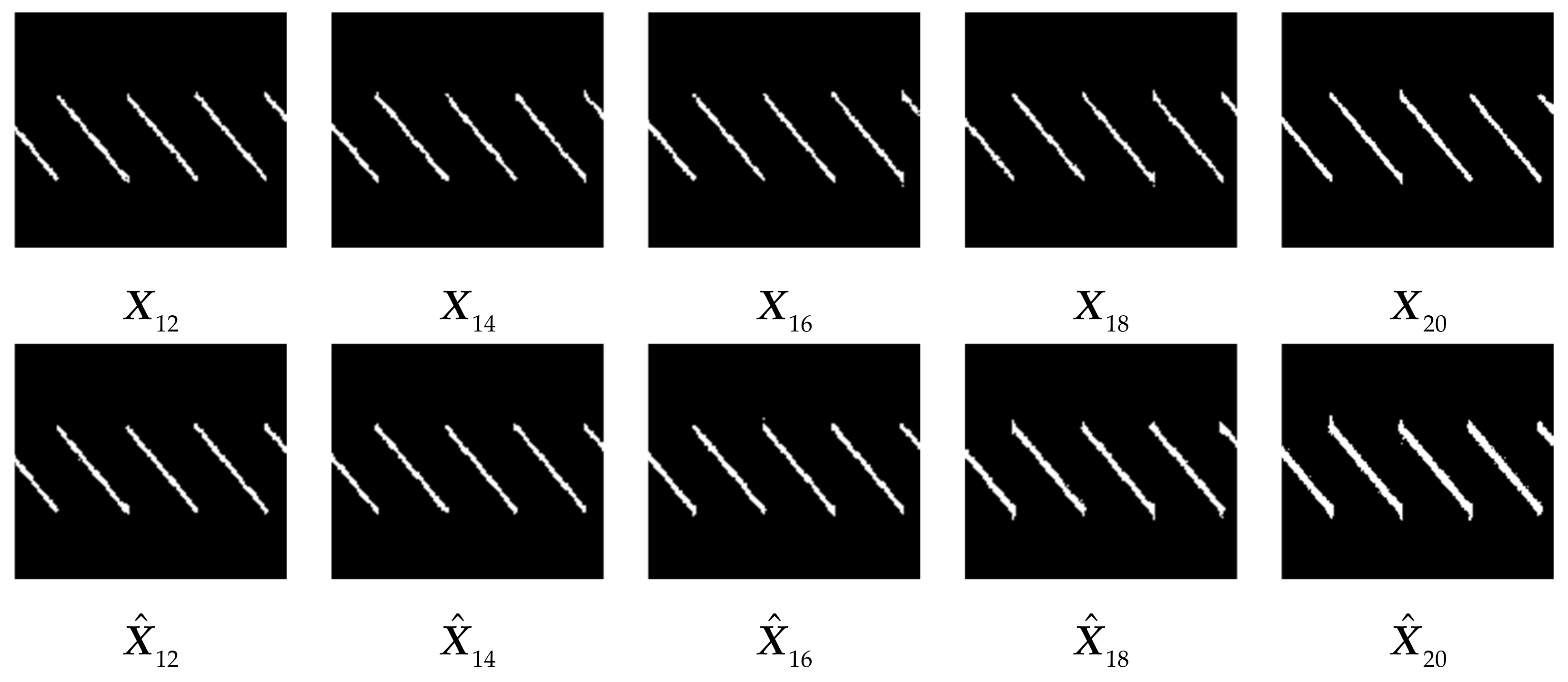
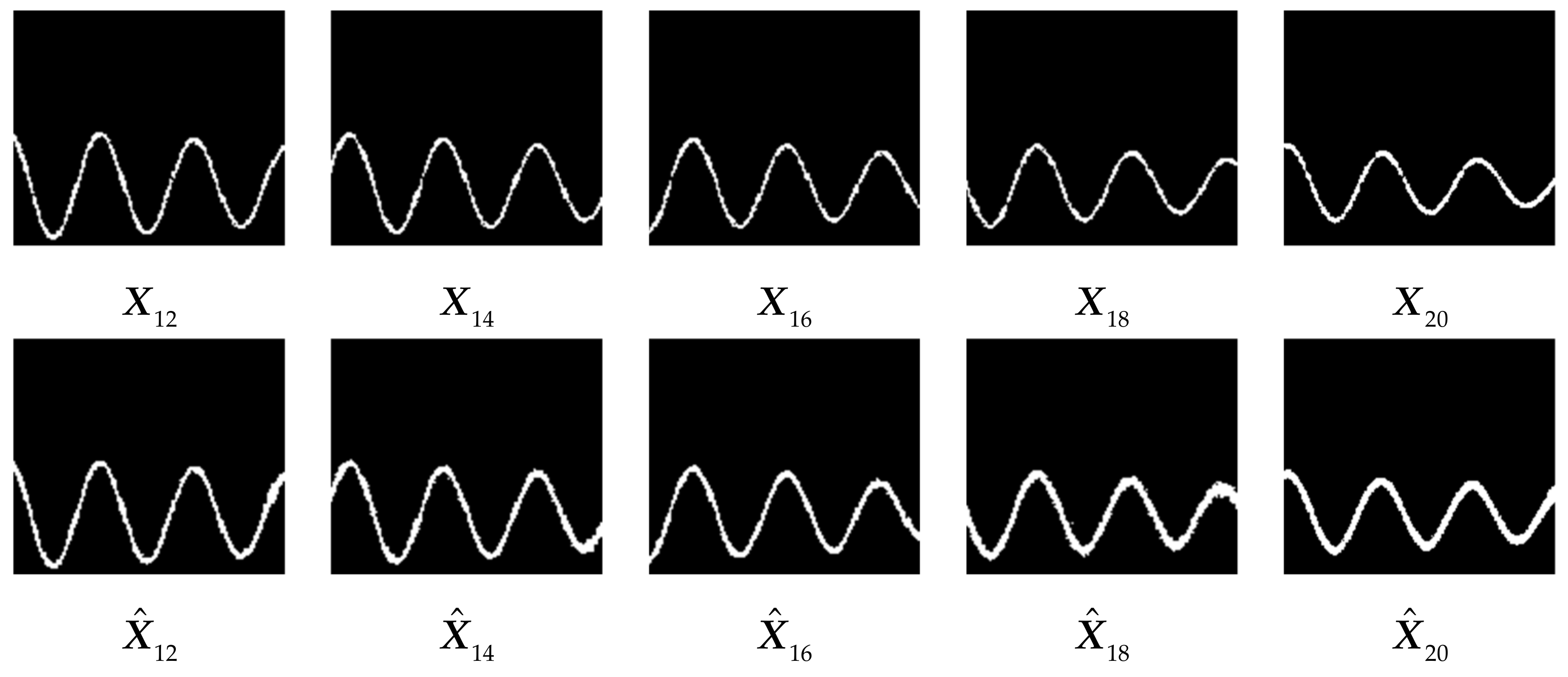
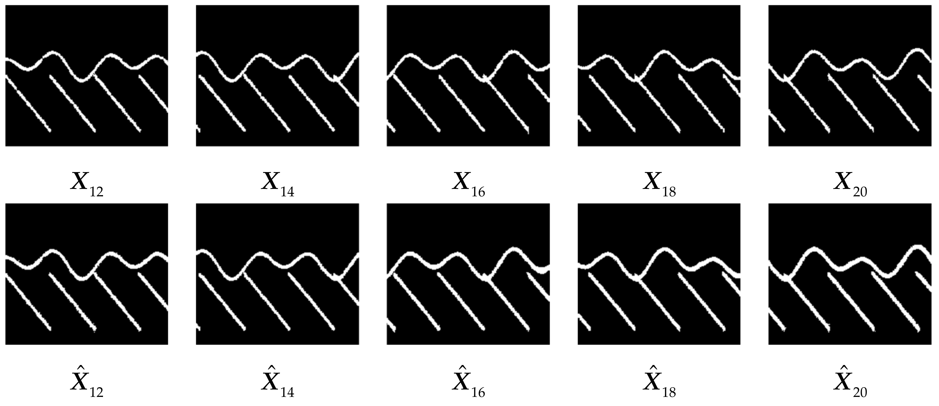
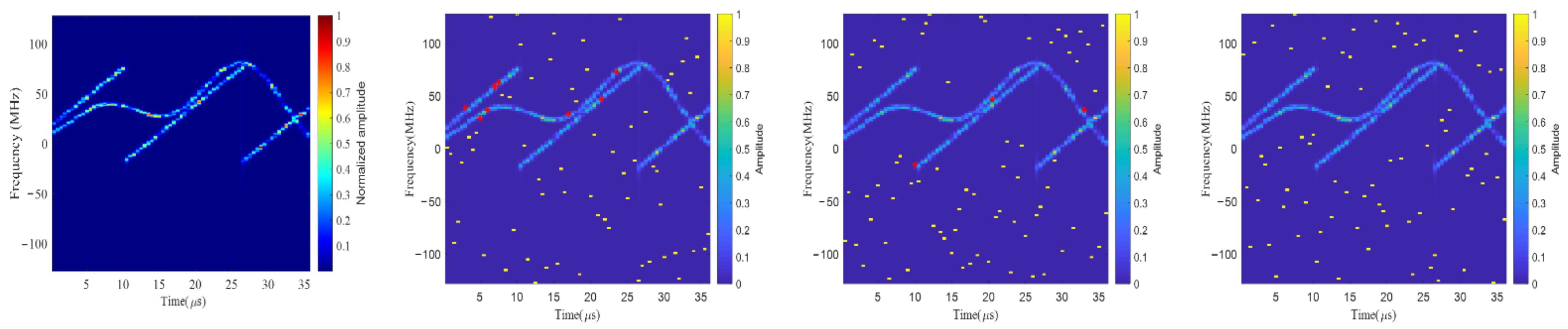
3.1. Prediction Results of Different WBIs

In this sub-section, we verify the performance of PredRNN for WBI prediction. To simulate the actual complicated WBI in practice, we model the WBI as the mixing of the chirp-modulated WBI (CM-WBI) and the sinusoidal-modulated WBI (SM-WBI) [26,27], expressed as

$$\begin{array}{c}I(t)=B_{CM}(t)\cdot \exp [j2\pi f_{CM}t+j\pi \mu {(t-(⌊t/T_{CM}⌋+0.5)T_{CM})}^2]\\ +B_{SM}(t)\cdot \exp [j2\pi f_{SM}t+j{\displaystyle {\sum }_{k=1}^K{\beta }_k\sin (2\pi f_{k}t+{\phi }_k)}]\end{array}$$

(26)

where T_CM denotes the period of the CM-WBI, f_CM and f_SM denote the carrier frequencies, μ denotes the chirp rate, β_k, f_k, and φ_k denote the amplitude, frequency, and phase of the k-th (k = 1, 2, …, K) sinusoidal signal of the SM-WBI, and with K as the number of sinusoids, B_CM(t) and B_SM(t) denote the modulation amplitudes, modeled as band-passed Gaussian noise signals with the standard deviations as I_CM and I_SM, which are determined by the interference-to-signal ratio (ISR).

With the parameters randomly selected from

Table 1. Value range of the simulated WBI parameters.

Parameter	Value Range	Parameter	Value Range
BCM	ISR = [40, 70] dB	BSM	ISR = [40, 70] dB
fCM	±[0, 50] MHz	K	{1, 2, 3}
TCM	[15, 20] μs	βk	[200, 500]
μ	±[4, 6] MHz/μs	fk	[0.02, 0.05] MHz
fSM	±[0, 40] MHz	φk	[−π, π]

, we generated 5000 WBIs based on (26) for PredRNN training. The duration of each WBI is set as 216.5 μs and the data sampling frequency is set as 256 MHz. We apply the STFT with a sliding Hamming window to generate the WBI TF image sequence, where the window size is 256 and the overlap length is 128. For each WBI, 20 overlapped TF images are obtained with ΔT = 8 μs, Ts = 64 μs, and thus V = U = 10. In Pytorch, the ADAM optimizer is used for PredRNN training with the learning rate as 5 × 10⁻⁴ and the batch size as 8. With 100,000 iterations, Figure 4 shows the training loss curve of PredRNN. It can be seen that the training loss of PredRNN is graduated reduced and becomes almost unchanged after 60,000 iterations, indicating the convergence of the training process. In the following, we take some testing experiments by the trained PredRNN.

With the input as $\underset{¯}{{\mathit{X}}_I}=〈{\mathit{X}}_1,{\mathit{X}}_2,\dots ,{\mathit{X}}_{10}〉$, Figure 5, Figure 6 and Figure 7 show the prediction results $\underset{¯}{{\widehat{\mathit{X}}}_O}=〈{\widehat{\mathit{X}}}_{12},{\widehat{\mathit{X}}}_{14},\dots ,{\widehat{\mathit{X}}}_{20}〉$ obtained by the trained PredRNN for three different testing WBIs, i.e., CM-WBI only, SM-WBI only, and the mixed WBI. It can be observed that, for all three different testing WBIs, PredRNN can predict the future WBI well. The predictions are consistent with the ground truth.

To quantitively assess the prediction performance of the trained PredRNN in different prediction lengths for different WBIs (i.e., CM-WBI only, SM-WBI only, and the mixed WBI), we calculate the mean squared error (MSE) of the u-th ($u=1,2,\dots ,10$) predicted TF image, expressed as

$$\mathrm{MSE}(u)=\frac{1}{It}{\displaystyle {\sum }_{it=1}^{It}{‖{\widehat{\mathit{X}}}_{V+u}^{it}-{\mathit{X}}_{V+u}^{it}‖}_F^2/D_X}$$

(27)

where It = 1000 is the testing number, $D_X$ is the number of all the elements of ${\mathit{X}}_{V+u}^{it}$.

The obtained MSEs are shown in Figure 8. It can be seen that the performance of WBI prediction improves with the decrease of the prediction length u, which is consistent with the fact that the shorter-time TF feature of the WBI can be more easily estimated from its historical ones. For different testing WBIs, the prediction performance decrease with the increase of the complexity of WBI. The prediction performance for CM-WBI is the highest and that for mixed WBI is the lowest.

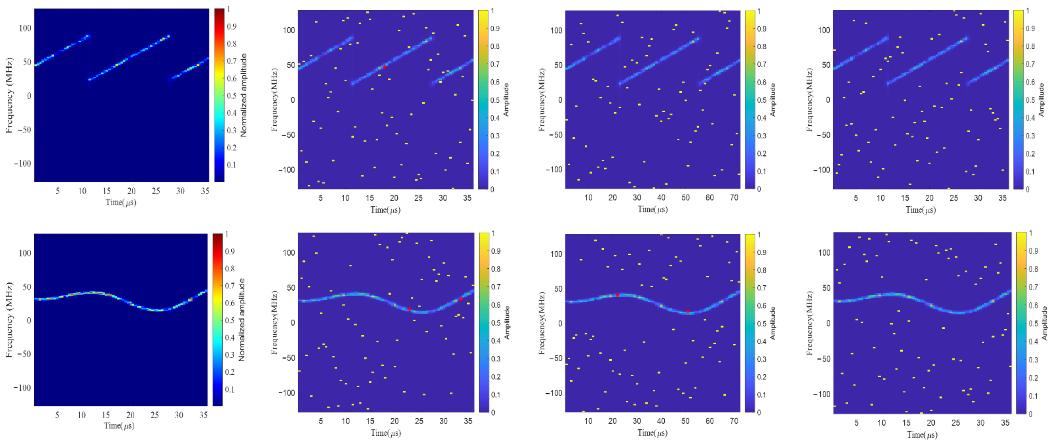
3.2. Imaging Results under Different WBIs

In this sub-section, we verify the performance of the proposed imaging method under different WBIs. The parameters of the 2D cross MIMO radar system are shown in

Table 2. 2D cross MIMO radar system parameters.

Parameter	Value
Tx/Rx antenna number	M = N = 36
Tx/Rx antenna spacing	dt = dr = 8 m
Center frequency	fc = 10 GHz
Frequency step	Δf = 2 MHz
Sub-pulse number	Q = 128
Sub-pulse duration	Ts = 0.5 us

, based on which Mu = Nu = 24 transceiving antennas and Qu = 72 sub-pulses are selected to construct the sparse MIMO radar system. Given a target that has P = 47 scattering points located at 10 km from the radar system, Figure 9a shows its 3D positions {x, y, z} = {[x₁,x₂,…,x_P], [y₁,y₂,…,y_P], [z₁,z₂,…,z_P]} relative to the reference point. Based on (8), Figure 9b shows the target parameters {α, β, χ} = {[α₁,α₂,…,α_P], [β₁,β₂,…,β_P], [χ₁,χ₂,…,χ_P]}. In the following, {α, β, χ} is used as the ground truth of target imaging for simplicity.

Given the ISRs of CM-WBI and SM-WBI as 70 dB and other parameters randomly selected from Table 1, Figure 10 shows the TF images of different WBIs in the duration of measurement and different transmitting RSSF waveforms. The first column of Figure 10 is the TF images of CM-WBI only, SM-WBI only, and the mixed WBI. The last three columns of Figure 10 are the TF images of the transmitting waveforms designed via random selection, the SWD method, and the proposed WBI prediction method. The red crosses in the TF images mark the frequencies that are overlapped with the WBI in the TF domain. In other words, the red crosses represent the interfered sub-pulses in the received signal.

It can be seen from Figure 10 that, as different sub-pulses will be interfered, the waveforms designed via random selection and the SWD method may work in the environment with simple and stationary WBI (e.g., CM-WBI only), but may be seriously affected when the WBI becomes more complicated (e.g., SM-WBI only and the mixed WBI). In real situations, the WBI is usually complicated. In such a case, the waveform designed via the proposed WBI prediction method is more effective to avoid the WBI influence.

Corresponding to Figure 10, Figure 11 shows the target imaging results obtained by different methods. For each row in Figure 11, the imaging results are obtained via random selection, WDR, SWD, and WBI prediction from left to right. For each column in Figure 11, the imaging results are obtained under CM-WBI only, SM-WBI only, and the mixed WBI from top to bottom. As indicated in Figure 11, with the increase of the WBI complexity, the imaging results obtained via random selection and SWD both degrade a lot. The SWD method can help to improve the performance of random selection, while the imaging results also degrade. Regardless of the increasing complexity of the WBI, the proposed method can always achieve a high image quality.

To assess the imaging results quantitatively, we calculate the normalized mean squared errors (NMSEs) and image contrasts (ICs) of different results in Figure 11 based on

$$\mathrm{NMSE}={‖\mathcal{X}-{\mathcal{X}}_0‖}_F/{‖{\mathcal{X}}_0‖}_F$$

(28)

and

$$\mathrm{IC}=\frac{\sqrt{\mathrm{Ave}\left\{{[|\mathcal{X}{|}^2-\mathrm{Ave}\left\{\right|\mathcal{X}{|}^2\}]}^2\right\}}}{\mathrm{Ave}\left\{\right|\mathcal{X}{|}^2\}}$$

(29)

where $\mathcal{X}$ denotes the target image obtained by different methods, ${\mathcal{X}}_0$ denotes the ground-truth image corresponding to the target parameters {α, β, χ} shown in Figure 9b, Ave{·} denotes the averaging operation for all the elements in an image.

Table 3. MSEs and ICs of the imaging results obtained via random selection (RND Sel.), WBI detection and removal (WDR), simple waveform design (SWD), and the proposed method.

	WBI	RND Sel.	WDR	SWD	Proposed
MSE (dB)	CM-WBI	−5.0816	−7.8354	−8.2236	−8.3893
	SM-WBI	4.8549	−6.8587	4.9389	−7.6529
	Mixed WBI	13.7198	−2.2180	3.1501	−7.0912
IC	CM-WBI	132.0076	156.2876	159.9774	159.1816
	SM-WBI	38.0723	156.6958	38.9409	159.3246
	Mixed WBI	23.5171	99.5433	47.5641	155.4871

shows the NMSEs and ICs of different methods, where the bolded values are the highest/lowest. The lower/higher the value of NMSE/IC, the better the image quality. It can be seen from Table 3 that, compared to other methods, the proposed method can always obtain high imaging performance.

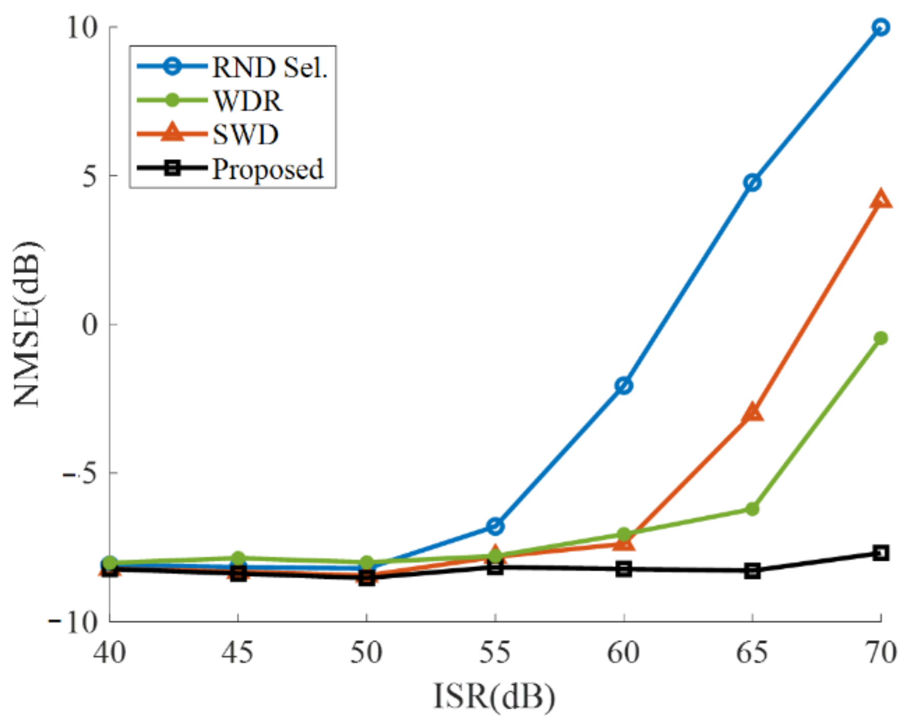
3.3. Robustness of the Proposed Method

To further compare the proposed method with others and show its robustness under different ISRs, 50 Monte Carlo trials were carried out for different methods under the same mixed WBI conditions, where the ISRs of CM-WBI and SM-WBI are both varying from 40 dB to 70 dB. For every trial, the WBI parameters are randomly from Table 1. The averaged NMSEs of different methods over 50 trials are calculated, giving the results shown in Figure 12. It can be learned from Figure 12 that: (1) the NMSEs of all the four methods increase with the ISR increases, (2) the NMSEs of all the four methods are nearly the same when the ISR is lower than 55 dB, (3) the NMSEs of random selection, the WDR method, and the SWD method increase quickly when the ISR increases from 55 dB to 70 dB, (4) the NMSEs of the proposed method are always the lowest compared to others and its NMSE increase is relatively small. These results indicate that, compared to other methods that degrade a lot when the ISR becomes high, the proposed method can always achieve a stable imaging performance under different ISRs.

At last, under the condition of the mixed WBI with the ISR fixed as 70 dB, two additional simulations are carried out to assess the robustness of the proposed method under different antenna/sub-pulse numbers and different signal-to-noise-ratios (SNRs). Firstly, keeping SNR = 0 dB and the relationship $M_u=N_u=Q_u/3$, we calculate the NMSEs of different imaging methods by changing the number of selected transmitting antennas M_u from 12 to 24 with a step of 2. With 50 Monte Carlo trials, the averaged results are shown in Figure 13a. Secondly, keeping $M_u=N_u=Q_u/3=24$, we calculate the NMSEs of different imaging methods by changing the SNR from −40 dB to 0 dB with a step of 5 dB. Similarly, the averaged results obtained with 50 Monte Carlo trials are shown in Figure 13b. It can be seen from Figure 13 that the proposed method can always achieve the smallest NMSEs, indicating its effectiveness and robustness under different conditions.

4. Discussion

With various simulation results shown in Section 3, we have verified the proposed sparse recovery imaging method with WBI prediction for MIMO radar. However, it should be noted that, as the PredRNN is trained with the simulated dataset that only includes two typical WBIs, i.e., CM-WBI and SM-WBI, the performance of the proposed method will degrade to some extent in practical applications, where more different types of WBIs may exist.

Actually, the two typical WBIs are considered mainly because they are widely used in existing studies. To make the derivation of the proposed method convenient, other types of WBIs are not considered in this study, resulting in the limitation of the established WBI dataset. Theoretically, the proposed method does not restrict to any specific types of WBIs because any WBI with spatiotemporal correlation features in the TF domain can be predicted by PredRNN. However, its prediction performance is dependent on the established dataset. If the dataset contains only the two typical WBIs, the trained PredRNN will not be able to perform very well for other types of WBIs, which is consistent with the principle of a neural network.

It is known that, to achieve wider applications, the training dataset for a neural net-work must be augmented to contain more scenarios. Thus, for PredRNN, to predict more WBI types accurately, the established dataset should be augmented. However, it should be noted that, based on the trained PredRNN with the two typical WBIs, the size of the newly added WBIs can be small and thus the retraining process will be easy, i.e., transfer learning can be used to solve this problem.

Besides, from the viewpoint of cognition, the proposed method can be categorized as belonging to the cognitive radar imaging approach. However, as only the historical WBI information is exploited, the proposed method is only cognitive to the environment, without the cognition to the target. If the target cognition technique is further applied to adaptively select the transceiving antennas and sub-pulses, a higher target imaging performance can be obtained for MIMO radar, which we will explore deeply in the future.

5. Conclusions

In this paper, we propose a 3D high-resolution imaging method for MIMO radar under the condition of wideband interference based on predictive neural network and sparse recovery. Compared to the imaging methods based on interference mitigation, the proposed method does not need to eliminate the interference component from the received signal, and hence can reduce the loss of target information. Compared to the imaging methods based on waveform design with the historical interference as the reference, the proposed method uses the predicted interference to guide the waveform design. Thus, it can be more adaptive and avoid the receiving of interference to a greater extent. Simulation results show the effectiveness, advantages, and robustness of the proposed method under different conditions.

References

1. Fishler, E.; Haimovich, A.; Blum, R.; Chizhik, D.; Cimini, L.; Valenzuela, R. MIMO radar: An idea whose time has come. In Proceedings of the 2004 IEEE Radar Conference, Philadelphia, PA, USA, 29 April 2004; pp. 71–78. [Google Scholar]
2. Bliss, D.W.; Forsythe, K.W. Multiple-input multiple-output (MIMO) radar and imaging: Degrees of freedom and resolution. In Proceedings of the Thirty-Seventh Asilomar Conference on Signals, Systems & Computers, Pacific Grove, CA, USA, 9–12 November 2003; pp. 54–59. [Google Scholar]
3. Ding, S.; Tong, N.; Zhang, Y.; Hu, X. Super-resolution 3D imaging in MIMO radar using spectrum estimation theory. IET Radar Sonar Navig. 2017, 11, 304–312. [Google Scholar] [CrossRef]
4. Ding, S.; Tong, N.; Zhang, Y.; Hu, X.; Zhao, X. Cognitive MIMO Imaging Radar Based on Doppler Filtering Waveform Separation. IEEE Trans. Geosci. Remote Sens. 2020, 58, 6929–6944. [Google Scholar] [CrossRef]
5. Feng, W.; Friedt, J.-M.; Nico, G.; Sato, M. 3-D Ground-Based Imaging Radar Based on C-Band Cross-MIMO Array and Tensor Compressive Sensing. IEEE Geosci. Remote Sens. Lett. 2019, 16, 1585–1589. [Google Scholar] [CrossRef]
6. Donoho, D.L. Compressed sensing. IEEE Trans. Inf. Theory 2006, 52, 1289–1306. [Google Scholar] [CrossRef]
7. Hu, X.; Tong, N.; Zhang, Y.; Huang, D. MIMO Radar Imaging with Nonorthogonal Waveforms Based on Joint-Block Sparse Recovery. IEEE Trans. Geosci. Remote Sens. 2018, 56, 5985–5996. [Google Scholar] [CrossRef]
8. Jiao, Z.; Ding, C.; Liang, X.; Chen, L.; Zhang, F. Sparse Bayesian learning based three-dimensional imaging algorithm for off-grid air targets in MIMO radar array. Remote Sens. 2018, 10, 369. [Google Scholar] [CrossRef] [Green Version]
9. Hu, X.; Feng, C.; Wang, Y.; Guo, Y. Adaptive Waveform Optimization for MIMO Radar Imaging Based on Sparse Recovery. IEEE Trans. Geosci. Remote Sens. 2020, 58, 2898–2914. [Google Scholar] [CrossRef]
10. Zhou, C.; Li, F.; Li, N.; Zheng, H.; Wang, R.; Wang, X. Improved eigensubspace-based approach for radio frequency interference filtering of synthetic aperture radar images. J. Appl. Remote Sens. 2017, 11, 25004. [Google Scholar] [CrossRef]
11. Li, D.; Liu, H.; Yang, L. Efficient time-varying interference suppression method for synthetic aperture radar imaging based on time-frequency reconstruction and mask technique. IET Radar Sonar Navig. 2015, 9, 827–834. [Google Scholar] [CrossRef]
12. Tao, M.; Zhou, F.; Zhang, Z. Wideband Interference Mitigation in High-Resolution Airborne Synthetic Aperture Radar Data. IEEE Trans. Geosci. Remote Sens. 2016, 54, 74–87. [Google Scholar] [CrossRef]
13. Liu, H.; Li, D.; Zhou, Y.; Truong, T.-K. Simultaneous Radio Frequency and Wideband Interference Suppression in SAR Signals via Sparsity Exploitation in Time–Frequency Domain. IEEE Trans. Geosci. Remote Sens. 2018, 56, 5780–5793. [Google Scholar] [CrossRef]
14. Ding, Y.; Fan, W.; Tao, M.; Zhang, Z.; Wang, L.; Zhou, F.; Lu, B. Wideband interference mitigation for synthetic aperture radar based on the variational Bayesian method. Signal Process. 2022, 198, 108581. [Google Scholar] [CrossRef]
15. Han, W.; Bai, X.; Fan, W.; Wang, L.; Zhou, F. Wideband Interference Suppression for SAR via Instantaneous Frequency Estimation and Regularized Time-Frequency Filtering. IEEE Trans. Geosci. Remote Sens. 2022, 60, 1–12. [Google Scholar] [CrossRef]
16. Wang, S.; Liu, Z.; Xie, R.; Ran, L.; Wang, J. MIMO radar waveform design for target detection in the presence of interference. Digit Signal Process. 2021, 114, 103060. [Google Scholar] [CrossRef]
17. Tierney, C.; Mulgrew, B. Adaptive waveform design for interference mitigation in SAR. Signal Process. 2021, 178, 107759. [Google Scholar] [CrossRef]
18. Shi, J.; Jiu, B.; Liu, Y.; Yan, J.; Liu, H.; Hu, L. Fast transmit waveform design method for interference mitigation in simultaneous multibeam MIMO scheme. Electron. Lett. 2016, 52, 1166–1168. [Google Scholar] [CrossRef]
19. Fan, W.; Zhou, F.; Tao, M.; Bai, X.; Rong, P.; Yang, S.; Tian, T. Interference Mitigation for Synthetic Aperture Radar Based on Deep Residual Network. Remote Sens. 2019, 11, 1654. [Google Scholar] [CrossRef] [Green Version]
20. Tao, M.; Li, J.; Su, J.; Wang, L. Characterization and Removal of RFI Artifacts in Radar Data via Model-Constrained Deep Learning Approach. Remote Sens. 2022, 14, 1578. [Google Scholar] [CrossRef]
21. Li, W.; Gan, Y.; Zhao, J.; Zou, K.; Zheng, Z. Joint waveform design of cognitive radar based on LSTM network in the presence of signal-dependent interference. J. Appl. Remote. Sens. 2021, 15, 37501. [Google Scholar] [CrossRef]
22. Qiu, W.; Zhou, J.; Zhao, H.Z.; Fu, Q. Fast sparse reconstruction algorithm for multidimensional signals. Electron. Lett. 2014, 50, 1583–1585. [Google Scholar] [CrossRef]
23. Feng, W.; Yi, L.; Sato, M. Near range radar imaging based on block sparsity and cross-correlation fusion algorithm. IEEE J. Sel. Top. Appl. Earth Obs. Remote Sens. 2018, 11, 2079–2089. [Google Scholar] [CrossRef]
24. Shawel, B.S.; Woldegebreal, D.H.; Pollin, S. Convolutional LSTM-based Long-Term Spectrum Prediction for Dynamic Spectrum Access. In Proceedings of the 2019 27th European Signal Processing Conference (EUSIPCO), A Coruna, Spain, 2–6 September 2019; pp. 1–5. [Google Scholar]
25. Wang, Y.; Long, M.; Wang, J.; Gao, Z.; Yu, P.S. Predrnn: Recurrent neural networks for predictive learning using spatiotemporal lstms. In Proceedings of the 31st International Conference on Neural Information Processing Systems, Long Beach, CA, USA, 4–9 December 2017; pp. 879–888. [Google Scholar]
26. Huang, Y.; Zhang, L.; Li, J.; Chen, Z.; Yang, X. Reweighted tensor factorization method for SAR narrowband and wideband interference mitigation using smoothing multiview tensor model. IEEE Trans. Geosci. Remote Sens. 2019, 58, 3298–3313. [Google Scholar] [CrossRef]
27. Huang, Y.; Liao, G.; Xiang, Y.; Zhang, Z.; Li, J.; Nehorai, A. Reweighted nuclear norm and reweighted Frobenius norm minimizations for narrowband RFI suppression on SAR system. IEEE Trans. Geosci. Remote Sens. 2019, 11, 5949–5962. [Google Scholar] [CrossRef]
Figure 1. The geometry of the considered 2D sparse cross MIMO radar system.
Remotesensing 14 03774 g001
Figure 2. The framework of the proposed sparse recovery imaging method with WBI prediction.
Remotesensing 14 03774 g002
Figure 3. The network structure of a L-layer PredRNN.
Remotesensing 14 03774 g003
Figure 4. The training loss of PredRNN versus the training iterations.
Remotesensing 14 03774 g004
Figure 5. The prediction results for CM-WBI. The first row shows the ground truth and the second shows the predicted results.
Remotesensing 14 03774 g005
Figure 6. The prediction results for SM-WBI. The first row shows the ground truth and the second row shows the predicted results.
Remotesensing 14 03774 g006
Figure 7. The prediction results for the mixed WBI. The first row shows the ground truth and the second row shows the predicted results.
Remotesensing 14 03774 g007
Figure 8. The WBI prediction performance of PredRNN against the prediction length for the chirp-modulated WBI (CM-WBI), the sinusoidal-modulated WBI (SM-WBI) and the mixed WBI.
Remotesensing 14 03774 g008
Figure 9. (a) The 3D position of the target and (b) the ground truth of target imaging.
Remotesensing 14 03774 g009
Figure 10. The TF images of different WBIs (CM-WBI only, SM-WBI only, and the mixed WBI from top to bottom) in the duration of measurement and the transmitting waveforms designed via different methods (random selection, the SWD method, and the proposed method from second to last column).
Remotesensing 14 03774 g010aRemotesensing 14 03774 g010b
Figure 11. The imaging results obtained by different imaging methods under different WBIs.
Remotesensing 14 03774 g011
Figure 12. NMSEs of different imaging methods against ISRs. The imaging methods are random selection (RND Sel.), WBI detection and removal (WDR), simple waveform design (SWD), and the proposed method.
Remotesensing 14 03774 g012
Figure 13. (a) NMSEs of different imaging methods against the numbers of selected antennas/sub-pulses and (b) NMSEs of different imaging methods against SNRs. The imaging methods are random selection (RND Sel.), WBI detection and removal (WDR), simple waveform design (SWD), and the proposed method.
Remotesensing 14 03774 g013