Sensing Requirements and Vision-Aided Navigation Algorithms for Vertical Landing in Good and Low Visibility UAM Scenarios

Abstract

To support the rapid development of the Urban Air Mobility framework, safe navigation must be ensured to Vertical Take-Off and Landing aircraft, especially in the approach and landing phases. Visual sensors have the potential of providing accurate measurements with reduced budgets, although integrity issues, as well as performance degradation in low visibility and highly dynamic environments, may pose challenges. In this context, this paper focuses on autonomous navigation during vertical approach and landing procedures and provides three main contributions. First, visual sensing requirements relevant to Urban Air Mobility scenarios are defined considering realistic landing trajectories, landing pad dimensions, and wind effects. Second, a multi-sensor-based navigation architecture based on an Extended Kalman Filter is presented which integrates visual estimates with inertial and GNSS measurements and includes different operating modes and ad hoc integrity checks. The presented processing pipeline is built to provide the required navigation performance in different conditions including day/night flight, atmospheric disturbances, low visibility, and can support the autonomous initialization of a missed approach procedure. Third, performance assessment of the proposed architecture is conducted within a highly realistic simulation environment which reproduces real world scenarios and includes variable weather and illumination conditions. Results show that the proposed architecture is robust with respect to dynamic and environmental challenges, providing cm-level positioning uncertainty in the final landing phase. Furthermore, autonomous initialization of a Missed Approach Procedure is demonstrated in case of loss of visual contact with the landing pad and consequent increase of the self-estimated navigation uncertainty.

1. Introduction

The term Urban Air Mobility (UAM) refers to the concept of a new transportation network which will enable the movement of people and goods in urban areas through short flights of innovative platforms, mainly represented by electrical Vertical Take-Off and Landing (VTOL) and Short Take-Off and Landing (STOL) aircraft. Currently, many efforts are focused on realizing a safe UAM framework including the potential development of advanced navigation technologies and algorithms, which will allow the aircraft to reliably perform critical flight procedures such as approaches and landing in urban scenarios. In this context, the conventional landing systems are expected to be complemented or replaced by technological solutions tailored to UAM, including the use of multiple exteroceptive sensors (e.g., cameras, radars, LIDARs) and, consequently, of multi-sensor navigation algorithms. Furthermore, the level of autonomy of the vehicles will increase with the aim to gradually remove the necessity for onboard pilots enabling higher payload capabilities, while ensuring safe operations in each flight phase [1]. This process will require the implementation of autonomous decision-making algorithms complementing the navigation estimates with piloting functions, such as the capability to decide for Missed Approach Procedures (MAP) if the conditions required to safely perform landing are not met. This paper studies the problem of vertical approach and landing procedures of VTOL aircraft in the frame of UAM scenarios. Context and state of the art are described in sub-Section 1.1. with reference to approach and landing procedures and visual based sensing solutions, while sub-Section 1.2 clarifies the paper contribution.

1.1. Context and Related Works

At the time of writing this paper, aviation authorities are starting to publish the first documents to design vertiports area and vertical take-off and landing procedures. The EASA has first issued the Special Condition VTOL [2] containing indications to prove compliance of VTOL aircraft prototypes with safety and design objectives, and then published the Prototype Technical Design Specifications for Vertiports [3], distinguishing two main types of Visual Flight Rules (VFR) for landing procedures:

• Conventional Landing (CL) with a defined glide path, which resembles the final phase of the VFR approach path to heliports [4] as well as the vertiports’ VFR approach procedure proposed by FAA in the Draft Engineering Brief for Vertiport Design [5];
• Vertical Landing (VL) with a defined obstacle-free volume (see Figures D-13 and D-14 of [3]), which will be required to maintain safe distances to obstacles in the airspace above vertiports placed in urban environments.

At the same time, the UAM literature has already identified many different approach and landing profiles compliant with the taxonomy provided above. Examples of the CL approaches are provided by [6,7]. These solutions ensure a constant glide path during the whole trajectory, with advantages such as the possibility to fly at higher velocities avoiding dangerous aerodynamic phenomena like the Vortex Ring State (VRS). Hence, they represent an optimal solution in terms of time and energy consumption in scenarios that allow a gradual descent to the landing pad, keeping safe distances to potential obstacles.

When this latter requirement cannot be met, as in complex urban areas, the approach and landing path should be selected, searching for a compromise between the constraints linked to aerodynamic and obstacle avoidance. In this respect, some approach solutions have been proposed, foreseeing a final vertical phase (according to the VL paradigm) in which the VTOL aircraft descends at a limited sink rate. For instance, the 3-stepped approach trajectory involves a descent with a fixed approach path until 200 m height above the vertiport, a horizontal forward flight to the point right above the landing pad, and a final vertical descent [8,9]. Such a vertical descent is also proposed in the Terminal Area of Multi-vertiport system Concepts of Operations [10]. An alternative trajectory is defined by Song et al. [11,12], who propose a vertiport airspace model, namely the Vertiport Terminal Control Area (VTCA), optimized to control the approach of the arriving aircraft through holding circles where the vehicles hover while waiting for the authorization to complete the landing procedure.

The above-presented vertical approach solutions are not compatible with the nominal visual slope indicators supporting VFR approaches, such as the Helicopter Approach Path Indicator (HAPI) lights, and with the glideslope/localizer guidance provided by the Instrument Landing Systems (ILS) adopted in Instrument Flight Rules (IFR) runway approaches, leading to the necessity of alternative means to estimate the relative position with respect the landing pad. Another issue is represented by the limited pilot view of the landing area due to the elevate slope, which can be addressed by means of synthetic cues like those obtainable by cameras according to the EASA [3].

Following these considerations, the implementation of a robust multi-sensor architecture exploiting relative pose estimates obtained processing the frames collected by cameras installed on the VTOL aircraft might represent a potential solution. Clearly, an efficient ground infrastructure has to be designed to also correctly detect the landing pad in non-nominal visibility conditions (e.g., bad weather and night scenarios) to support the defined architecture and, in particular, the visual-based pose estimation task.

In the framework of small UAS landing, the recognition of the landing pad has been applied for H-shaped patterns placed in cluttered scenarios in nominal visibility conditions [13] and in the case of low-illumination environments [14]. An alternative vision-only method relies on the detection of ArUco markers placed in correspondence to the landing point, demonstrating an accuracy of 11 cm in outdoor environments [15]. Usage of InfraRed (IR) cameras allow the extension of vision-based pose estimation techniques to night scenarios. For instance, a flight controller receiving input pose estimates from the detection of an IR-illuminated fiducial marker, as well as LIDAR and Inertial Measurement Unit (IMU) measurements, is presented in [16]. Another approach identifies roof ledges through Convolutional Neural Network, enabling reliable pose estimates for autonomous UAV landing [17]. Deep Learning-based pose estimates are integrated with IMU measurements for autonomous navigation based on Visual-Inertial Odometry in [18], also showing a landing spot detection technique achieving an accuracy better than 10 cm.

The adoption of vision-aided navigation solutions has been studied also for larger rotorcraft in the UAM landing framework. In [19], a vision-only method is presented based on the autonomous detection of an H-shaped landing site in the last 25 m of the VL trajectory of a VTOL aircraft, providing position estimates with an accuracy of 1.5 m. Another study extends the vision-based pose estimation approach to the initial part of the approach phase, through the integration in an Extended Kalman Filter (EKF) of the IMU measurements and the pose estimates computed recognizing a pattern of lights placed in the surroundings of the landing pad [20]. However, the approach trajectory with a constant glide descent of 9° (similar to the procedures proposed by FAA [4,5,7]) considered in the latter work might result not feasible in complex scenarios with high buildings in the area around the landing pad, and the defined lights pattern (covering a 50 m-by-350 m area) might not be integrable in urban scenarios which have a limited space available for the vertiport area.

1.2. Paper Contribution

In this framework, this paper provides the following contributions:

• The definition of the visual sensor requirements needed to safely support these operations and increase the autonomy of the navigation architecture. Considering the case of low visibility conditions, this corresponds to extending the sensing requirements of Enhanced Visual Operations (EVO) to the new UAM scenarios.
• The implementation of a vision-aided, multi-sensor-based navigation architecture which integrates the measurements of an IMU, a standalone GNSS receiver, and a monocular camera. A multi-mode data fusion pipeline based on an EKF is designed, which takes the distance from the landing area into account and adopts ad hoc strategies to self-estimate navigation performance degradation and improve integrity, protecting the navigation solution and consequently the overall landing procedure from visual sensing anomalies.
• Performance assessment of the proposed architecture is conducted within a highly realistic simulation environment in which sensor measurements are realistically reproduced, analysing day/night scenarios in both nominal and low visibility conditions. Given the stringent safety requirements of UAM operations, the scope of this analysis is to understand how the developed logic and processing pipeline work in degraded conditions, and which are the applicability limits of the developed concepts.

The next Section defines the requirements to adopt vision sensors to complement/substitute the pilot role in approach and landing phases. The requirements will be defined based on aspects such as the assumed approach trajectory, the dimensions of the landing pad and the aerodynamic constraints which influence the aircraft path in case of wind fields. Section 3 will present the proposed navigation architecture, and the visual pose estimation algorithm selected. Section 4 describes the customized simulation environment designed to test the navigation architecture. Section 5 presents the results of simulations conducted to validate the proposed architecture and analyse the performance under highly variable visibility conditions. Finally, conclusions are reported in Section 6.

2. Visual Sensor Requirements in UAM Landing Scenarios

Visual sensors can be installed on VTOL platforms to support navigation and control functions which are usually relegated to the onboard pilot. In the approach and landing phases, the collected camera frames can be processed to detect and track the landing pad, and estimate the vehicle relative position. While visual sensors can also be used to provide Sense and Avoid capabilities with respect to fixed and moving obstacles, the following analysis does not address these issues and focuses on navigation and control needs in the terminal flight phases.

2.1. Assumptions

A preliminary literature analysis relevant to approach and landing operations in UAM scenarios is conducted to quantify the vision sensor’s requirements as a function of the possible aspects that might influence them. Three main features are addressed: approach and landing trajectories; landing pad dimensions; wind field effects.

Regarding the first point, the literature reported in Section 1 shows that there are two different Concepts of Operations that can be selected. The choice between a constant glide path and a vertical approach path has an impact on visual sensor requirements such as the camera mounting configuration and Field of View (FOV). As reported by the EASA [3], VTOL aircraft may need to be equipped with ad hoc sensing systems, e.g., cameras, to safely perform vertical take-off and VL procedures without losing the visual cues needed by the pilot in these phases. In this paper, as in most of the recent literature, the focus is set on VL approaches, and the considered trajectories are the 3-stepped approach path and the VTCA. As it happens for helicopter Point in Space (PinS) operations, a clear definition of the “visual flight phase”, in which the visual contact with the landing pad must be established, is also needed in these approach procedures. The Transition Point to the Visual Flight phase (TPVF) (Figure 1) is placed at 350 m distance from the vertiport, which is consistent with the performance of the autonomous vision-based algorithm for landing pad detection and pose estimation reported is Section 5. The heights of the defined transition points are conformal to the minimum height (Decision Height at minimum 250 ft) required to obtain Visual Meteorological Conditions in current helicopter PinS procedures [21].

Figure 1. (a) 3−stepped trajectory and selected TPVF (highlighted in red); (b) VTCA trajectory and selected TPVF (highlighted in red).

With regards to the second point, the following areas can be defined around the landing pad, extending the regulations from the heliport design literature [3,5,22].

• Touch-down and Lift-off Area (TLOF), i.e., the load bearing surface on which the aircraft lands and/or takes off. Its minimum length and width should be at least equal to the distance between the two outermost edges of the vehicle according to the FAA [5] or to the diameter of the smallest circle enclosing the VTOL aircraft projection on a horizontal plane, as stated by the EASA [3] for elevated TLOFs. The TLOF can be designed to be rectangular or circular. According to the FAA, different advantages are provided by the two design choices. A rectangular TLOF provides better guidance for the pilot, while a circular TLOF may result more visible in an urban environment. The TLOF is assumed with a diameter of 12.2 m (40 ft) [7], coherently with the dimensions of the main VTOL prototypes, which are foreseen to be certified for UAM procedures [23].
• Final Approach and Take-off Area (FATO), which is centred around every TLOF area. This area represents the surface where VTOL aircraft complete the final phase of the approach to a hover or a landing. It is assumed that the minimum horizontal dimensions of this area are 1.5 times the minimum diameter of the circle enclosing the VTOL aircraft projection [3]. A more conservative definition of the FATO dimensions is provided by the FAA [5], assuming twice the distance between the vehicle’s two outermost edges.
• Safety Area (SA), which is defined on a heliport surrounding the FATO to reduce the risk of accidents for aircraft inadvertently diverging from the FATO.

The dimensions of the landing pad (i.e., the TLOF) impact both the required sensors’ FOV and resolution to keep the landing point clearly defined in the imagery during the visual phase of the vertical landing path.

Finally, aiming to define the safety requirements to adopt vision sensors in UAM approach and landing scenarios, an important role is given to urban wind field effects.

The risk for vehicles to encounter wind gusts in urban environments with high levels of turbulence is increased with respect to nominal high-altitude operations. In the proximity of extended high-rise buildings, VTOL aircraft flights might be affected by sudden wind gusts generated by the interaction of the turbulent airflow with the buildings [24]. The evaluation of the vehicle reaction to urban gusts, both with a pilot in command or an onboard autonomous guidance system, allows understanding if there is the risk to overcome the Required Obstacle Clearance (ROC) limits. The required vision sensor FOV has to consider these effects to maintain the visual contact with the landing pad during the whole approach and landing procedure to avoid the necessity to perform a MAP. A preliminary assessment of the effects of low altitude urban gusts on UAVs has been reported by Galway et al. [25], although focused on UAVs lighter than the vehicles that are predicted to be operative in UAM scenarios, estimating parameters such as the maximum attitude oscillations that the rotorcraft can experience in this situation (i.e., ±15° yaw and ±5° pitch for 8 kt background wind).

Moreover, wind fields determine the capability of safely taking off and landing along predefined directions, impacting VTOL aircraft dynamics, and inducing to impose constraints for approval of vertiport operations. These wind-related constraints are quantified for UAM scenarios by Zelinski [26] based on the experience of helicopter pilots:

• Rotorcraft should not attempt approach and departure operations with a tailwind, which can cause the aircraft to enter into VRS conditions.
• Rotorcraft should not attempt approach or departure operations with a crosswind greater than 15 knots.

These two constraints define the availability of vertiport TLOF pads according to the wind conditions, leading to the necessity to provide real-time estimates of the urban microclimates [1] and pre-schedule multiple paths according to the wind direction for single-pad vertiports. The VTOL aircraft during the departure and landing phases could be forced to maintain an attitude profile (changing the vehicle heading) to ensure that the relative wind speed is kept within the defined constraints while flying the standard trajectories. In that case, the possibility to perform an approach without exactly pointing the vertiport is a factor to be considered in the definition of vision sensor requirements in terms of FOV selection.

2.2. Requirements

A preliminary definition of the vision system requirements needed to reproduce pilot functions during approach and landing procedures can be obtained through the previous assumptions and the following considerations.

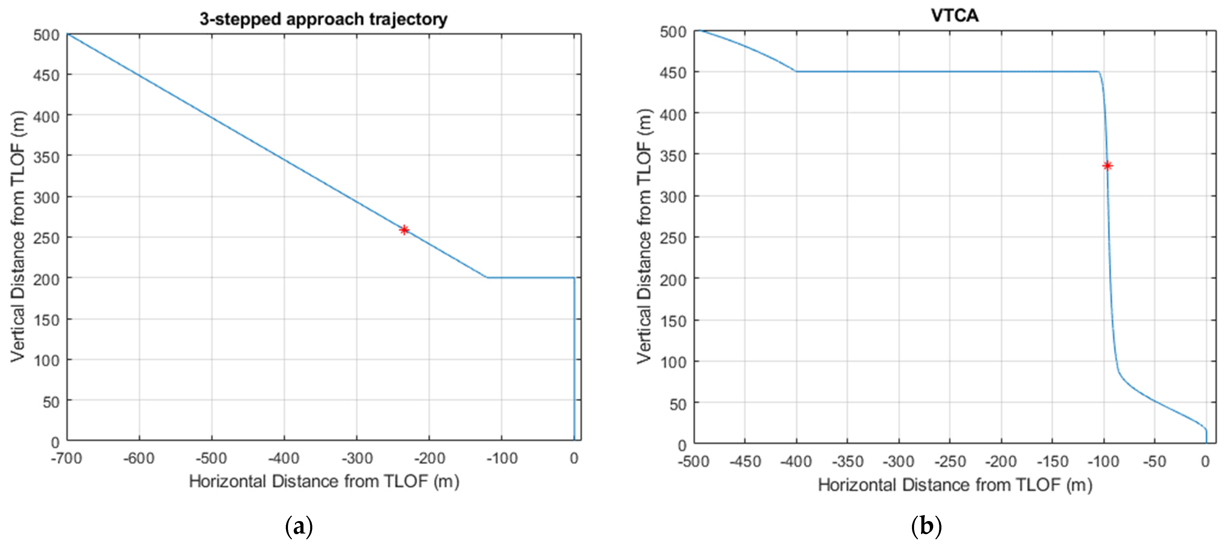
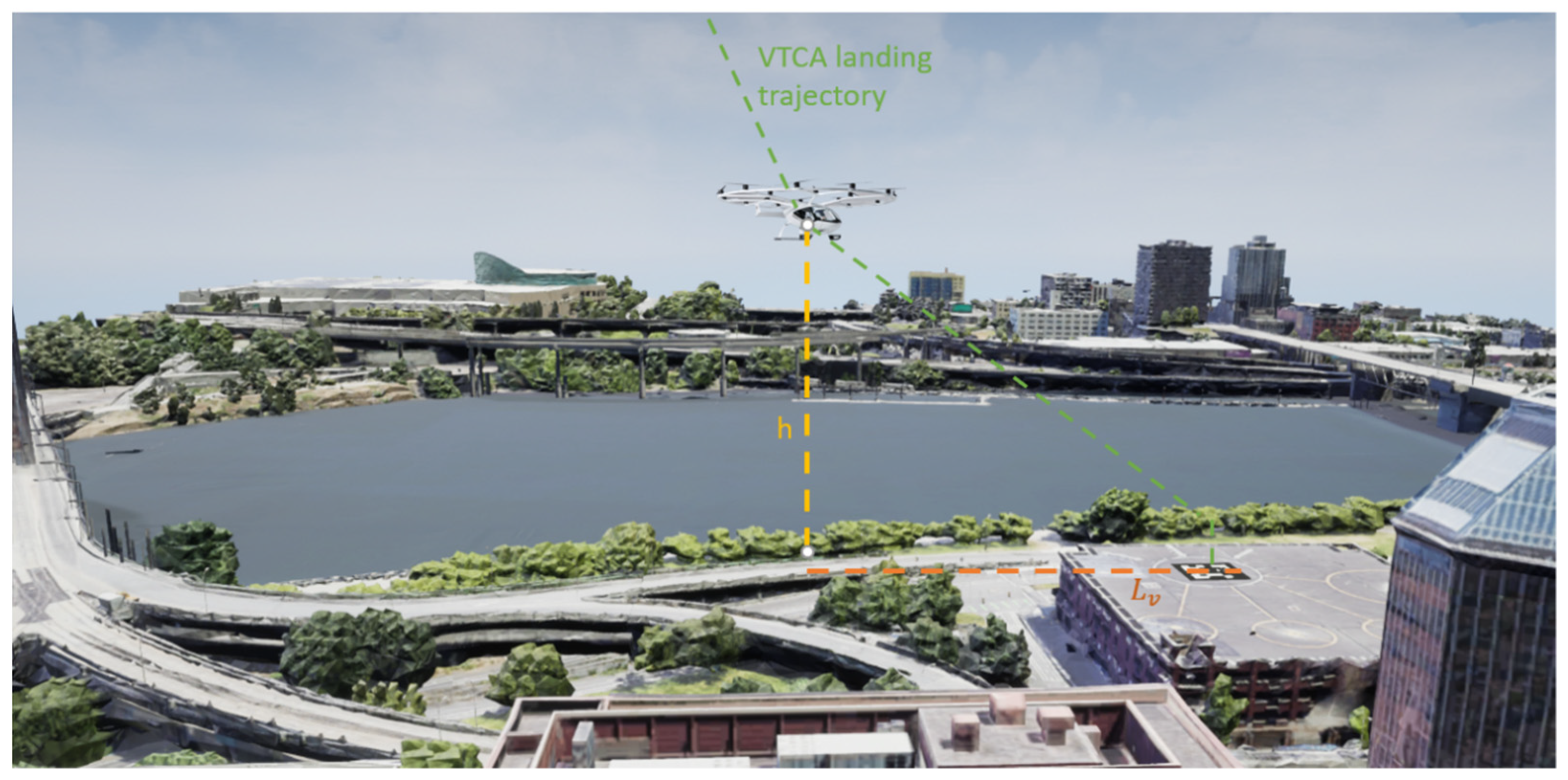
• Camera mounting configuration and FOV. For the considered type of approach trajectory, the camera must be mounted with an off-nadir pointing configuration. Moreover, different constraints can be identified on the field of regard to be monitored in the directions transversal and parallel to the velocity projection on the local horizontal plane, which determine different requirements for the camera horizontal and vertical FOV, respectively. Among the various impacting factors, the dimension of the landing pad and the wind direction and intensity play a crucial role. The minimum camera Horizontal FOV (HFOV) is defined to maintain visual contact with the TLOF area in the case of approaches in crosswind conditions producing a maximum heading deviation of 25°, and to exclude the risk of visual contact loss due to wind gusts causing a maximum heading oscillation of 15° of amplitude (as in [25]). Clearly, this implies that the landing procedure should be aborted if these conditions cause larger deviations from the nominal path. Consequently, using a worst-case approach, the resulting minimum HFOV is 80° (i.e., ±40°). The minimum camera Vertical FOV (VFOV) is estimated to maintain the landing pad in view during the visual flight phase of both the approach trajectories, considering the possibility of pitch oscillations (assuming max. ±5° as in [25]). The landing pad must be visible in the vision sensor imagery when the VTOL is in the final vertical descent above the vertiport and in each other point of the trajectories. Considering both the trajectories, the last holding circle of the VTCA is the point with the lower ratio between relative height and horizontal distance from the landing pad. The minimum VFOV required is defined through the comparison of the VFOV needed in this point to detect the landing pad and the value needed with the same camera mounting configuration during a vertical descent. It can be estimated by applying the pinhole camera model under perspective projection geometry, as in:

  $$\mathrm{VFOV} =2\times ta{n}^{-1} \left(\frac{Lv }{2 \ast h} \right)$$

  (1)

  where Lv is the maximum horizontal distance from the landing pad, while h is the vertical distance from the landing pad (Figure 2). Since h is 90 m while Lv can be computed as in:

  $$Lv=a+\frac{\mathrm{TLOF}}{2}$$

  (2)

  where a, i.e., the horizontal distance from the centre of the landing pad, is equal to 86.1 m while TLOF is 12.2 m, the minimum required VFOV would be 54.2°. Therefore, the required VFOV shall be at least 60° to consider also the assumed potential pitch oscillations. The simulations reported in Section 5 demonstrate that a camera with the above-defined FOV applied mounted with 20° pitch deflection from the nadir can provide a continuous visual contact with the landing pad in both the approach trajectories.
  

  Figure 2. Scheme of the defined parameters used to compute the required VFOV in the last holding circle of the VTCA landing trajectory (not in scale).
• Sensor resolution. Assuming the landing pad detection as the main objective of the selected camera to support the approach phase, the required sensor resolution will be strongly dependent on the ground infrastructure installed on it. Considering the previously reported TLOF dimensions (12.2 m × 12.2 m), a value of 0.05° Instantaneous Field of View (IFOV) leads to cover the area of interest with more than 1400 pixels at the TPVF defined along the approach trajectories. As better highlighted by the numerical simulation results shown in Section 5, this value results in being sufficient to accurately extract a fiducial marker placed in correspondence of the TLOF and visible in the whole approach trajectory, as well as to ensure an acceptable pose estimation accuracy.
• Refresh rate. The image frames shall be refreshed at least at 15 Hz, considering the nominal frame rates adopted in the vision-aided navigation sensor literature (20 Hz is tested in [14,16,17]) and the minimum 15 Hz value requested in nominal helicopter synthetic/enhanced/combined vision operations to runways [27]. Assuming a value of 25 m/s (90 km/h) for the maximum VTOL velocity as reported by the Volocopter VoloCity specification [23], the platform would travel a distance of about 1.56 m between two consecutive frame acquisitions. On the other hand, a higher refresh rate might be required in different applications which are characterized by higher platform speeds, for example the preliminary proof of concept of the eXternal Vision Systems (XVS) designed to support future supersonic operations providing real-time imagery in each flight phase assumes a camera frame rate of 60 Hz [28].
• System latency. A value of 100 m s is the maximum value considered acceptable in case of synthetic images presented to the pilot in rotorcraft landing operations [29]. This latency can be assumed as the threshold in these applications, including in the 100 m s value the latencies of the image processing and any sensor fusion phases. The assumed latency would lead the VTOL platform to fly 2.5 m between the frame acquisition and the end of its processing in the worst case of maximum flight speed assumed as before. Higher latency times might introduce the risk of pilot/autopilot oscillations.

Table 1 summarizes the defined vision sensor requirements.

Table 1. Summary of the estimated requirements to implement vision sensors in UAM approach and landing scenarios.

Vision Sensor Parameter	Required Value
Field of View	80° × 60°
Instantaneous Field of View	0.05°
Refresh rate	15 Hz
Maximum system latency	100 ms

3. Vision-Aided Navigation Architecture

As stated before, the previously defined camera requirements provide a continuous visual contact with the landing pad in the vertical approach trajectory. The acquired frames can be processed through vision-based algorithms to estimate the pose of the VTOL aircraft with respect to the landing pad. These pose measurements can then be fed into a filtering scheme according to a loosely coupled configuration.

The implemented navigation filter is based on a complementary EKF which estimates the state error vector based on the processing structure presented in [30], with the filter correction step relying on position estimates from both the GNSS and the visual algorithms. The navigation state components components are the Euler angles ψ, θ, φ, the velocity $v_N$, $v_E$, $v_D$ and the position components in North East Down coordinates with respect to the landing pad. The inertial navigation equations allow the propagation of the above-defined state vector. The integration of the visual-based pose estimation block in a closed-loop EKF architecture (Figure 3) provides remarkable advantages to the navigation performance during the approach flight phase.

Figure 3. Scheme of the multi-sensor architecture.

The main features of the architecture are reported below:

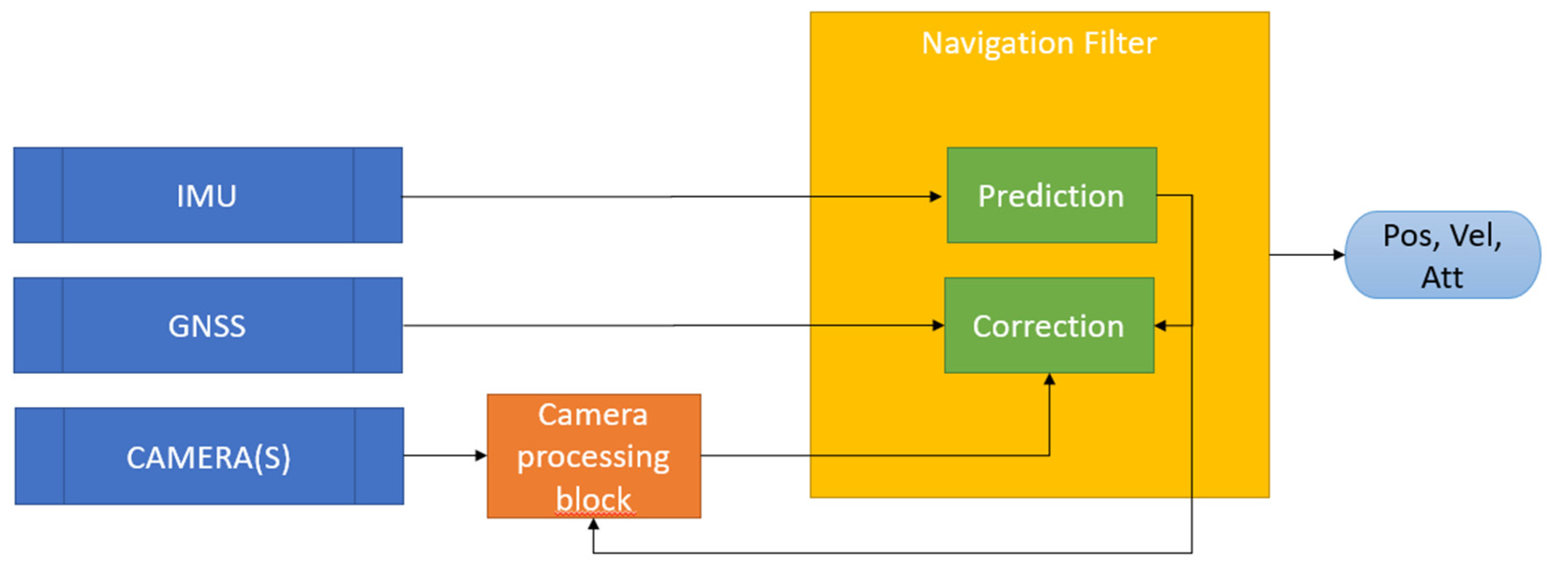
• The prediction step of the filter allows coping with the lower update rate of visual-based and GNSS-based measurements with respect to the inertial sensors data rate, thus ensuring valid initial guesses to the vision-based iterative pose estimation algorithm.
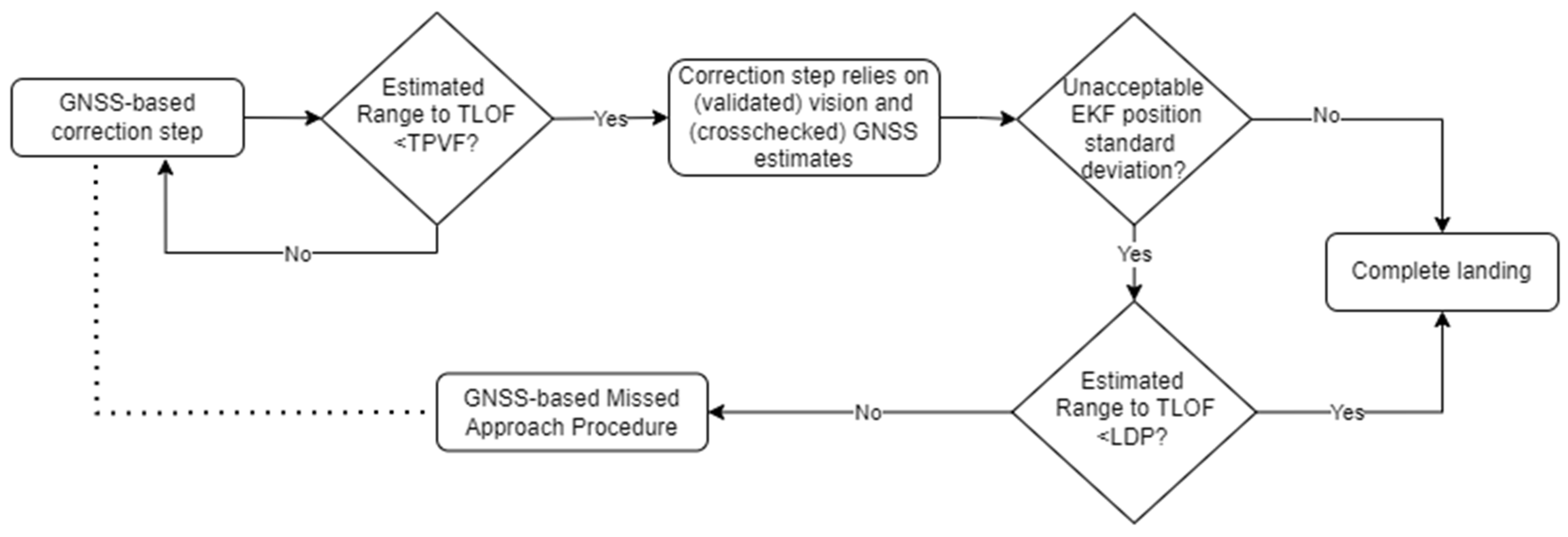
• The correction step of the filter in the approach phase trusts visual estimates and GNSS measurements for position data (Figure 4). Only the estimates provided by the standalone GNSS receiver are used in the first phase of the approach, when the high distances from the landing pad prevent from obtaining accurate markers’ detection, thus leading to coarse visual-based pose measurements. However, in this part of the approach path, the landing pad is already searched and tracked by the visual algorithm, thus being able to initialize the pose estimation process. Once the previously identified distance threshold from the landing pad (i.e., the TPVF) is reached, visual-based pose measurements are fed to the filter correction step. Specifically, in this second part of the approach, a multi-sensor correction step is implemented following the cascaded single-epoch integration model [30], combining both GNSS and visual sensor estimates. This scheme allows us to cross-check the integrity of GNSS measurements, which in urban scenarios might be affected at low altitudes by failures due to signal multipath or non-line-of-sight (NLOS) receiver [31]. The implemented logic accepts only GNSS position measurements that are included in the 3-sigma bounds defined over the corresponding filter position prediction through the uncertainties of the prediction and the measurement.
  

  Figure 4. Flowchart of the EKF correction step algorithm.
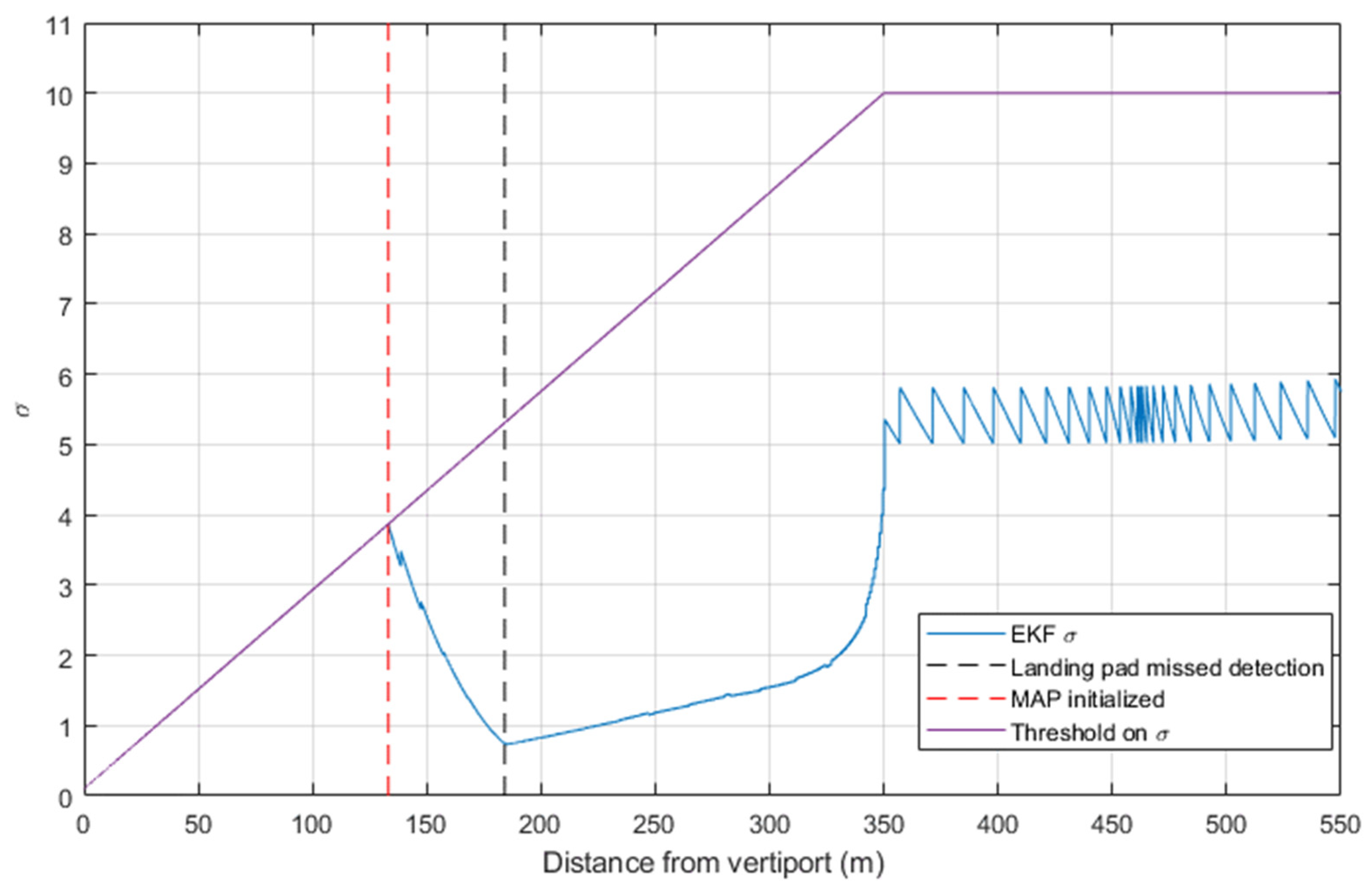
• Navigation performance is monitored at each time step through the control of the estimated position uncertainty of the EKF. To improve integrity, a failure detection logic verifies if the visual-based pose estimates are acceptable comparing the pose estimation residuals with a threshold. Thanks to this process, if the pose estimated from a specific image frame is deemed unreliable, it is not fed to the EKF correction step, thus not contributing to the reduction of EKF position error covariance. In a similar way, a missed detection of the landing pad in the image frame (e.g., due to unfavorable visibility conditions or to obstacles) does not provide visual position estimates. When the estimated navigation uncertainty, as expressed by the covariance matrix of the filter, reaches a threshold which is deemed not compatible with a safe landing procedure, a contingency event is generated with consequent activation of a MAP. As concerns the definition of the error thresholds for MAP activation, different approaches are possible which are all linked to the entries of the covariance matrix. As an example, within an ILS-like perspective, constant lateral and glide-slope deviation thresholds in degrees can be considered, and positioning uncertainties can be converted into angular deviations by taking the distance to the landing pad into account. For the sake of concreteness, in this work the threshold is set on the three-dimensional positioning uncertainty computed as the square root of the sum of the diagonal entries of the covariance matrix relevant to aircraft positioning. The threshold is assumed to have a linear dependence on the distance to the vertiport, which is consistent with the idea of a constant threshold for the angular errors. This choice is also in line with typical performance of visual sensors capable of providing improved position accuracy at reducing range. Since the logic adopted for MAP activation is based on the positioning uncertainty, the system behaviour is strongly affected by the characteristics of the inertial sensors. In fact, enhanced resilience with respect to visual challenges is provided by architectures, integrating higher performance inertial sensors which allow slower divergence of positioning errors. This is modelled by the smaller process noise matrix adopted in the navigation filter. It is worth noting that this is a navigation-induced MAP activation logic. In closed-loop autonomous landing operations, a MAP may also be activated by excessive control errors. These aspects are beyond the scope of this paper as the focus here is placed on perception and estimation aspects. In general, a sufficient battery charge must be available on electric VTOL aircraft to successfully cancel the landing procedure and divert to an alternate vertiport [32]. It is assumed that the possibility to perform a MAP shall be dependent on the VTOL aerodynamic performance and the scenario surrounding the vertiport, influencing the minimum distance from the landing pad at which it will be possible to safely cancel the landing procedure observing the ROC minima. Such distance corresponds to the Landing Decision Point defined by the EASA [3] and is assumed equal to 100 m in this work.

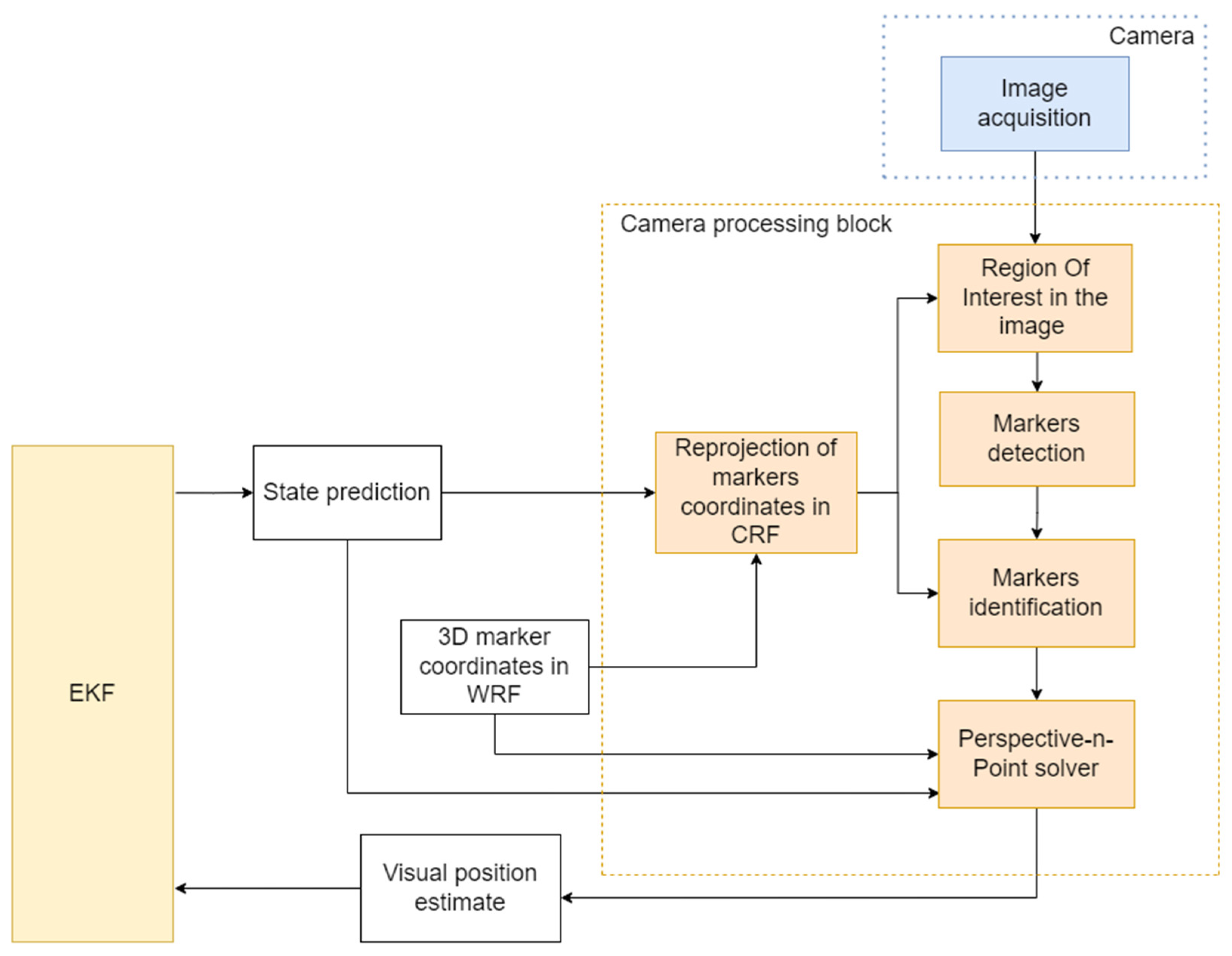
Visual-Based Pose Estimation

The role of the camera processing block within the above-defined architecture (in Figure 3) is to provide accurate estimates of the relative position of the VTOL aircraft with respect to the landing pad (Figure 5).

Figure 5. Flowchart of the camera processing algorithm.

Firstly, the collected image frames are processed to correctly detect and identify the fiducial markers placed in correspondence to the landing pad. To detect the markers, a region of interest is identified in each acquired frame, reprojecting the real coordinates ${\overline{x}}_{WRF}$ of the markers in the Camera Reference Frame (CRF) through the VTOL aircraft position ${\overline{p}}_{WRF}$ and orientation estimated at each prediction step by the filter. The orientation provided by the EKF is adopted to compute the rotation matrix ${\stackrel{=}{m}}_{321}$ from WRF to CRF needed to calculate the markers coordinates ${\overline{x}}_{CRF}$ at the single frame, as in:

$${\overline{x}}_{CRF}={\stackrel{=}{m}}_{321}\times \left({\overline{x}}_{WRF}-{\overline{p}}_{WRF}\right)$$

(3)

In that way, the image area to be processed to extract the markers of interest is reduced to a specific window containing all the estimated reprojections at each frame. The following markers (Figure 6) are selected in our study:

Figure 6. (a) AprilTag markers configuration; (b) Lights pattern.

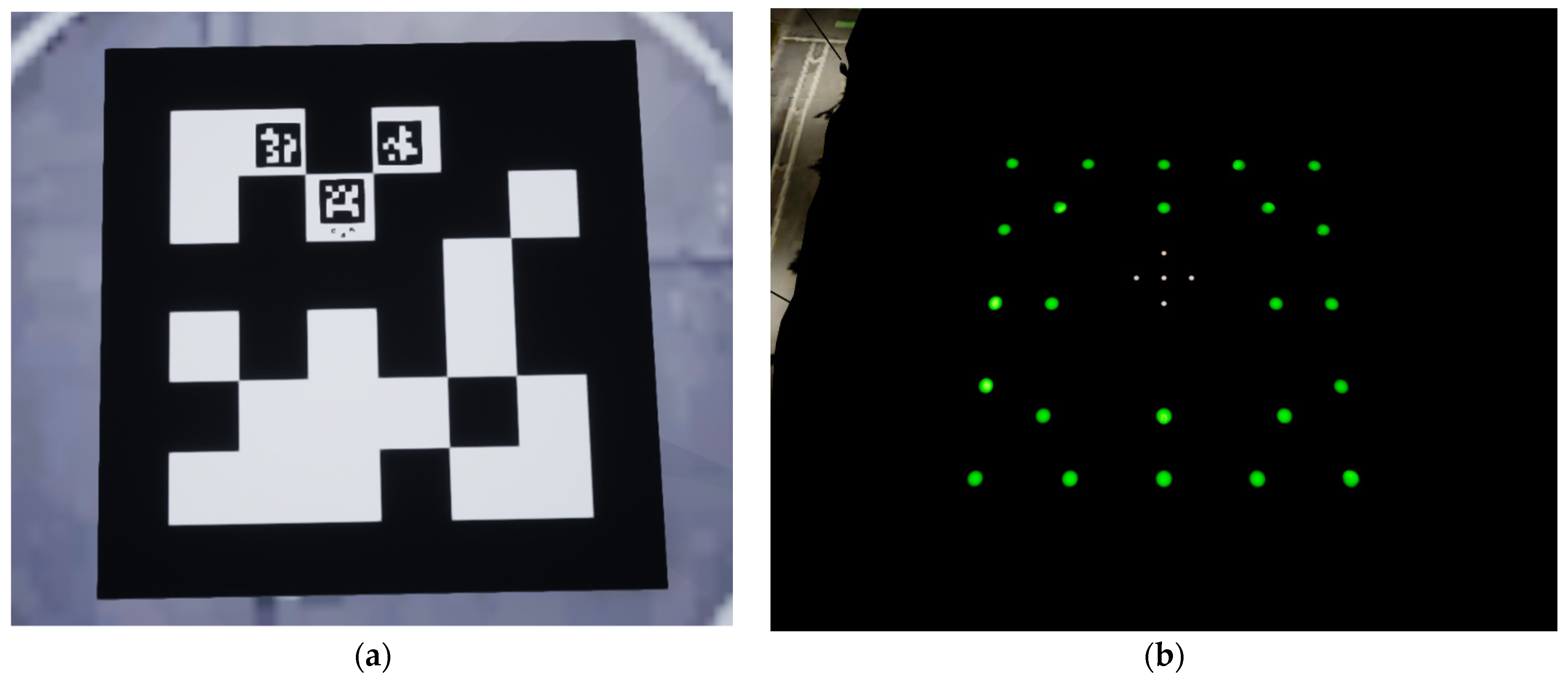
• AprilTag (AT) fiducial markers for daylight operations. A first AT marker occupying the TLOF area is placed on the landing pad to allow the pose estimation process at large distances, while 6 smaller ATs are adopted to maintain enough markers detectable in proximity of the landing pad. The smaller ATs are inserted into the first one thus not affecting the total landing pad dimension. The detection and identification of the AT markers is carried out exploiting the procedure presented in [33], implemented in MATLAB by the readAprilTag function.
• A pattern of lights for night scenarios respecting the FAA normative on heliport lighting [4] and the EASA specifications for vertiport design [3], including only the green flush lights placed in the FATO and TLOF areas to reduce the area occupied. The introduction of five white lights inside the TLOF area allows keeping reliable visual pose estimates in the last meters of the landing trajectory (similarly to the function of the 6 smaller ATs). Each light is identified minimizing the sum of the differences between the 2D coordinates of the green and white lights detected in the region of interest and the reprojection of the pattern’s real coordinates in the image plane. The defined Global Nearest Neighbour identification problem is solved by the Jonker-Volgenant [34] algorithm implemented in MATLAB by the assignkbest function.

Following the image processing and markers identification algorithms, the VTOL aircraft pose is estimated from the computed set of 2D–3D correspondences solving the Perspective-n-Point (PnP) problem. The selected technique for the solution of the PnP problem is a custom implementation of the iterative Levenberg–Marquardt (LM) algorithm, according to the formulation proposed by Gavin [35]. This solver receives a tentative pose guess in input, and iteratively minimizes the corner reprojection errors through least squares. The integration of the LM in the EKF permits to maintain accurate first guesses provided by the propagation of filter prediction through the IMU measurements. In that way, the iterative algorithm results are almost not influenced by sudden pose changes, providing fast and accurate pose estimates given in input to the EKF in the correction step with the related covariance. These covariance estimates are computed as in [36] through the Hessian matrix of the process, calculated from the Jacobian matrix J(x) of the 2D input coordinates $x_i$ transformation and uploaded in each iteration of the LM algorithm. The Hessian matrix $\stackrel{=}{A}$ is estimated as in:

$$\stackrel{=}{A}={\sum }_i(J^T\left(x_i\right)\times J\left(x_i\right))$$

(4)

and covariance matrix $\stackrel{=}{\mathsf{\Sigma }}$ is estimated through:

$$\stackrel{=}{\mathsf{\Sigma }}={\sigma }_n^2\times {\stackrel{=}{A}}^{-1}$$

(5)

where ${\sigma }_n^2$ is the variance of the additive Gaussian noise, related to the pixel-level uncertainty in the detection of to the fiducial markers on the image plane.

4. Simulation Environment

This Section introduces the simulation environment which has been developed to test the performance of the proposed navigation filter. The Portland heliport and its surroundings have been recreated in the gaming simulation environment Unreal Engine (UE) 4 to reproduce a potential scenario that might be selected for future flight test activities (Figure 7). The area covered by the reproduced scenario is 2 km × 2 km, which is considered adequate to analyse each phase of the simulated landing trajectories (Figure 1). The height above the terrain of the heliport selected for the landings is 24 m.

Figure 7. Unreal Engine 4 reproduction of the Portland heliport and its surroundings.

UE 4 permits to customize the scene model, through the introduction of fiducial markers or light patterns in correspondence of the selected landing site (see Figure 6). Moreover, the same simulation environment can be visualized changing the sun position in the sky sphere, emulating day/night/dusk conditions (Figure 8a), and weather conditions, e.g., adding fog (Figure 8b) or rain.

Figure 8. (a) UE4 reproduction of Portland heliport and its surroundings at night; (b) UE4 reproduction of Portland heliport and its surroundings with fog.

The MATLAB/Simulink UAV Toolbox allows the simulation of a rotorcraft flying in this UE scene with the sensors of interest installed on board. The adopted Simulink model (Figure 9) allows the control of the following aspects.

Figure 9. Implemented Simulink model, from the UAV Simple Flight Model of the Simulink UAV Toolbox.

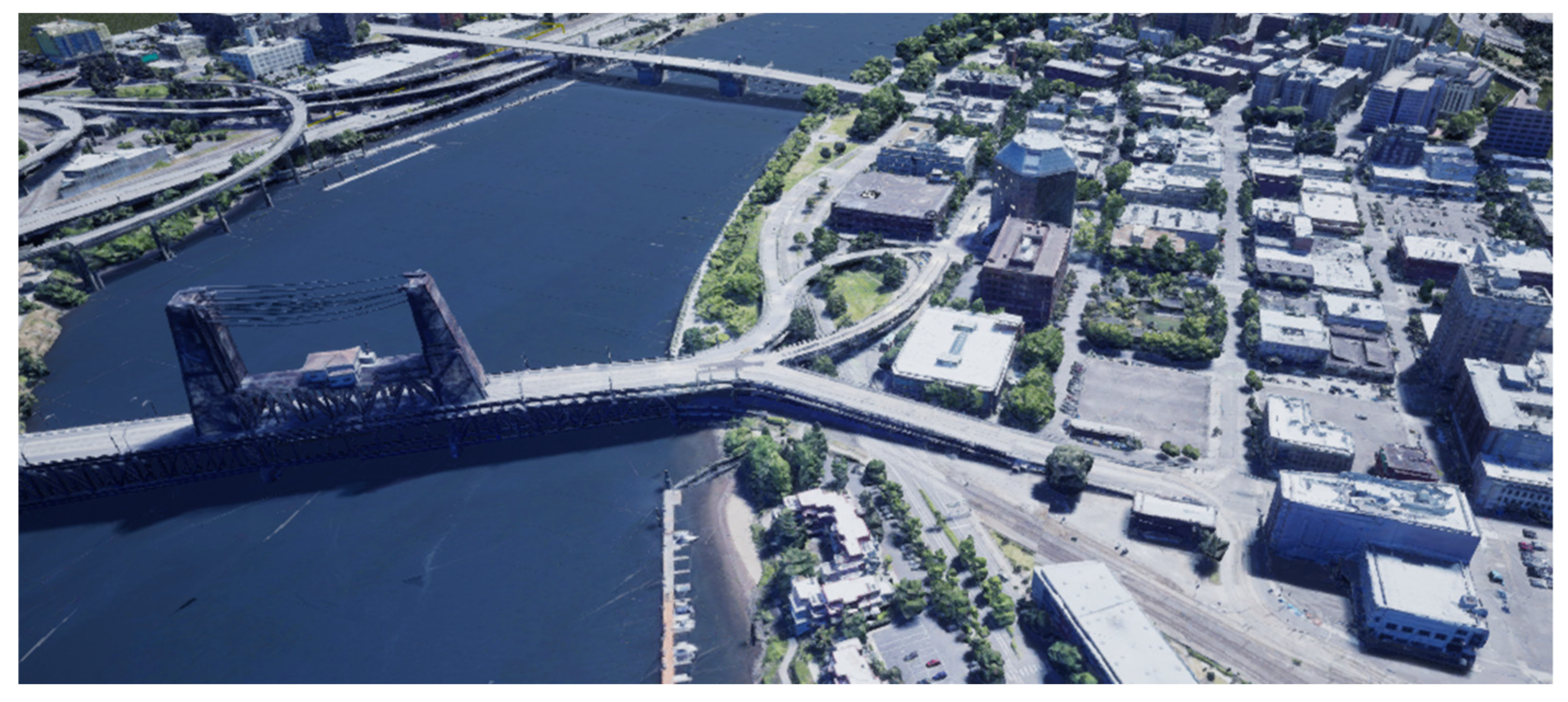
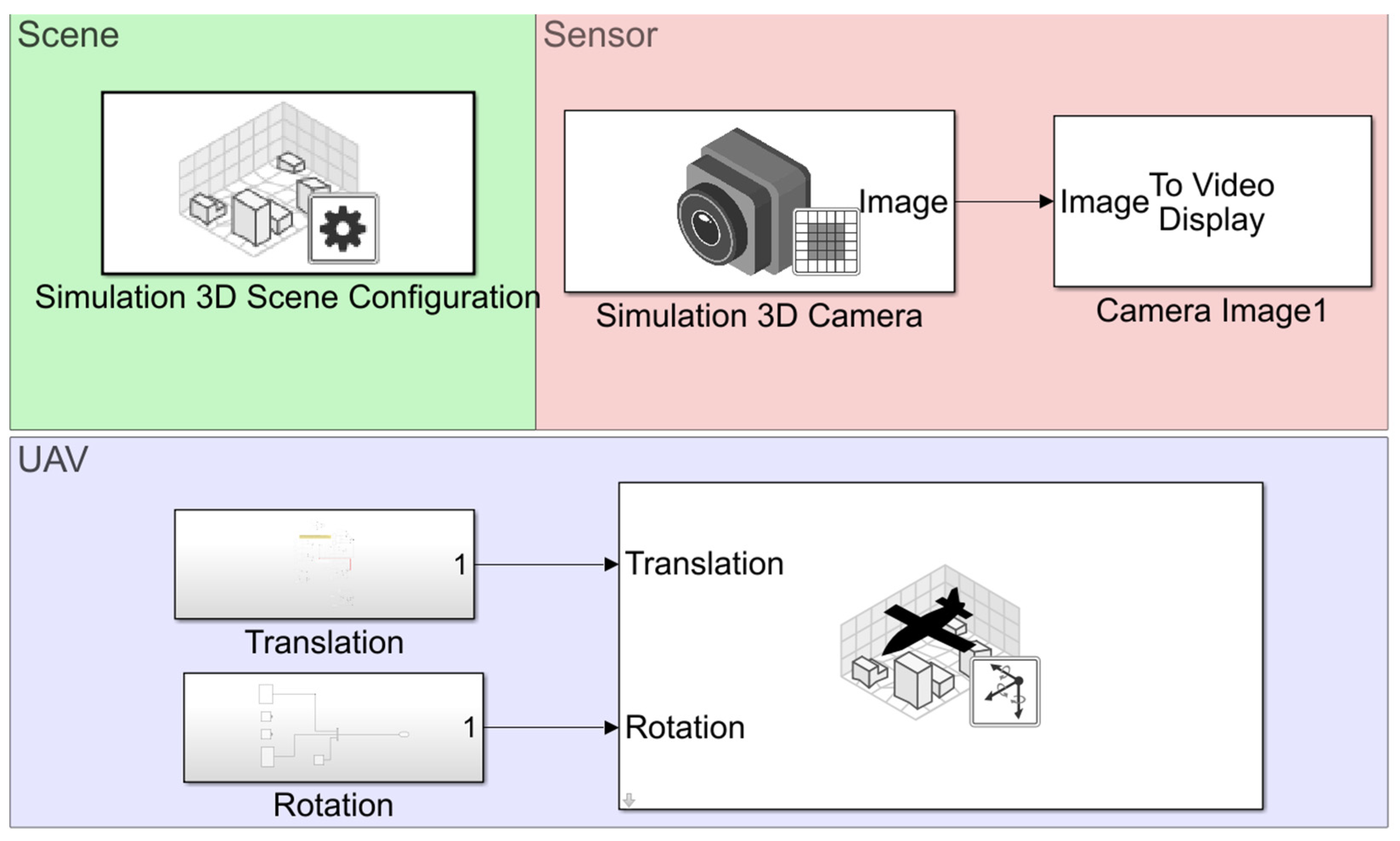
• The 3D scenario where the UAV flies, with the possibility to customize it through the interaction with UE changing weather and illumination parameters (as the Sun altitude and azimuth, the fog density, the cloud density, and speed). Furthermore, other UAVs flying in the scenario can be introduced, e.g., enabling the simulation of Sense and Avoid functionalities. Another effect on the scenario is given by the shadows of the simulated UAVs.
• The trajectory of the UAVs introduced in the scenario. It is worth noting that the simulated approach paths are the ideal ones reported in Section 5. Hence, the navigation estimates are not used to correct potential deviations from the ideal path through feedback control. At the moment, the effect of residual control errors is emulated through sinusoidal orientation and translation deviations of the ideal trajectory, while the effective introduction of feedback control in the trajectory simulations will be tacked in future applications.
• The parameters of the sensors installed on the rotorcraft, with the possibility to select nominal camera, fisheye camera, and LIDAR.

The specifications of the selected sensors are reported in Table 2. The GNSS receiver and the IMU are simulated through Matlab functions which receive in input the specifications reported in Table 2 and the imposed UAV trajectory. The GNSS’ position estimates and IMU’s accelerations and angular velocities estimates obtained in this way are randomly generated at each simulation respecting the assumed sensor properties. To simulate the acquired image frames, a video of the UAV flying in the selected scenario is recorded and subsequently converted into the single image frames.

Table 2. Specifications of the simulated sensors.

Simulated Sensor	Specifications	Selected Value
Camera	Focal length (pixels)	(1109, 1109)
	Principal point coordinates (pixels)	(808, 640)
	Image size (pixels) Sample frequency Off-nadir angle	(1280, 1616) 15 Hz 20 deg
GNSS receiver	GNSS Position Standard Deviation	2.5 m Horizontal–5 m Vertical
	Sample frequency	1 Hz
IMU	Sample Frequency	200 Hz
	Gyroscopes Angular Random Walk (ARW)	0.05 deg/sqrt(h)
	Gyroscopes Bias Instability (BI)	0.6 deg/h
	Accelerometers Velocity Random Walk (VRW) Accelerometers Bias Instability (ABI)	0.6 m/s/sqrt(h) 0.50 mg

5. Results

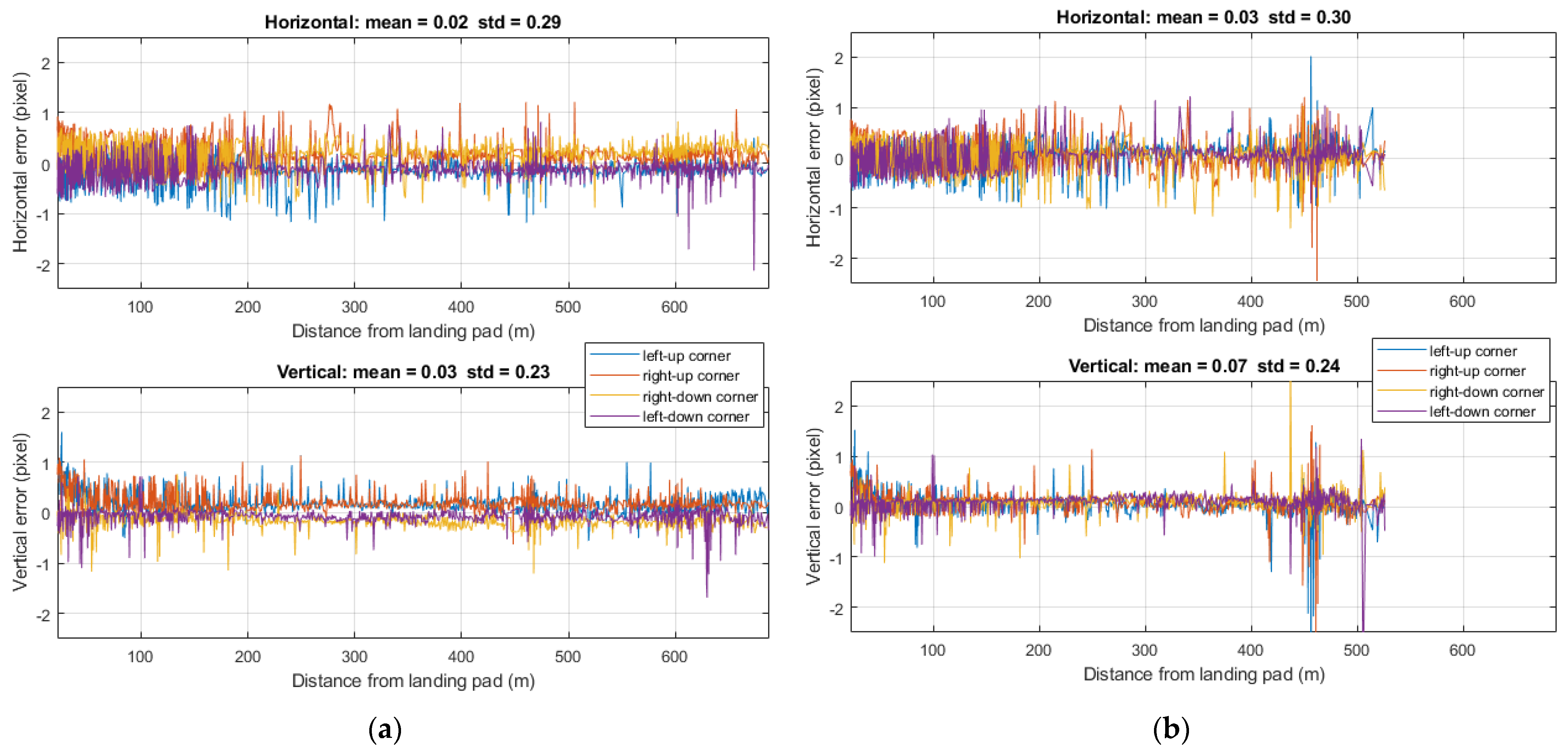
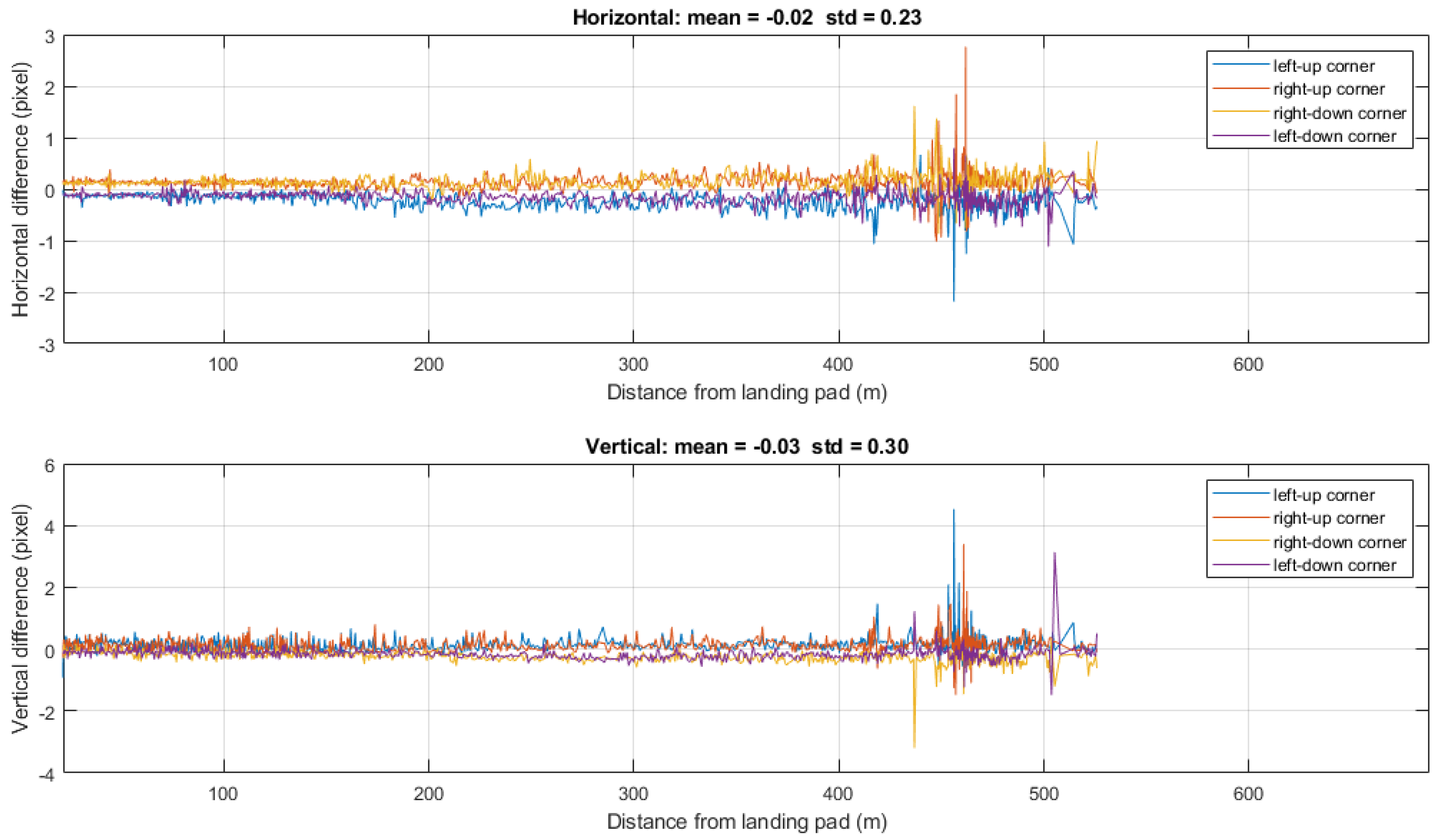
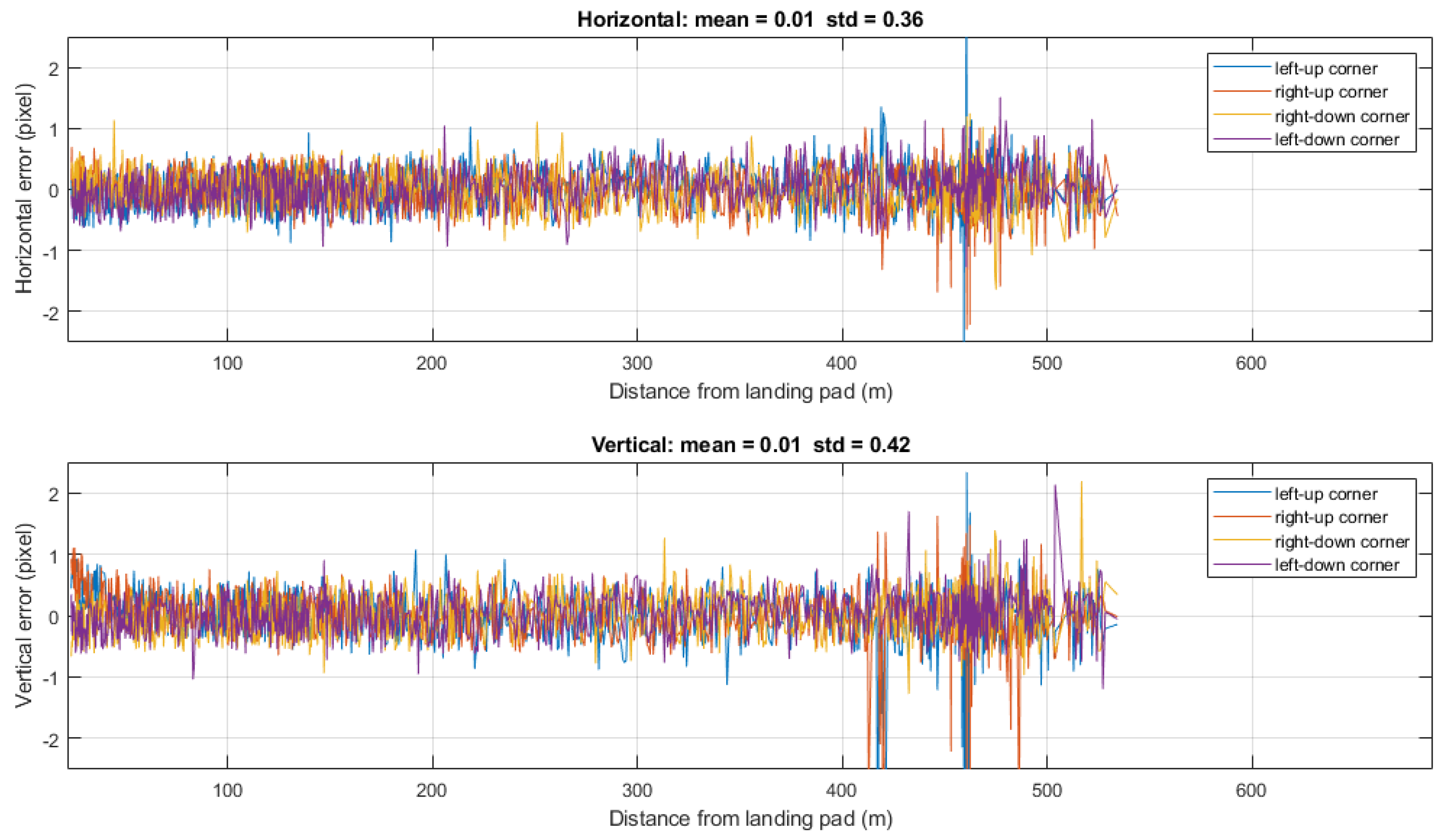
5.1. Visual-Based Pose Estimation Performance

Firstly, the performance of the implemented camera processing block has been tested to determine the accuracy of the position estimates provided by the LM algorithm. Figure 10 reports the positioning errors of the LM algorithm computed over 50 simulations of the same VTCA landing trajectory at daylight in nominal visibility conditions. The variability characterizing the simulations for this test case and the following ones is relative to the generation of IMU and GNSS measurements which are affected by random noise sources. The obtained errors confirm that a distance of 350 m can be assumed for the TPVF defined in Section 2, in which the filter correction step can include position estimates from the visual algorithm.

Figure 10. LM position estimates errors average over 50 simulations and 3−sigma bounds. VTCA landing trajectory in nominal visibility conditions. The plot scale is increased in the last 150 m to better show the errors in the final phase of the approach. The 350 m distance (black vertical line) from the landing pad is the selected threshold for TPVF.

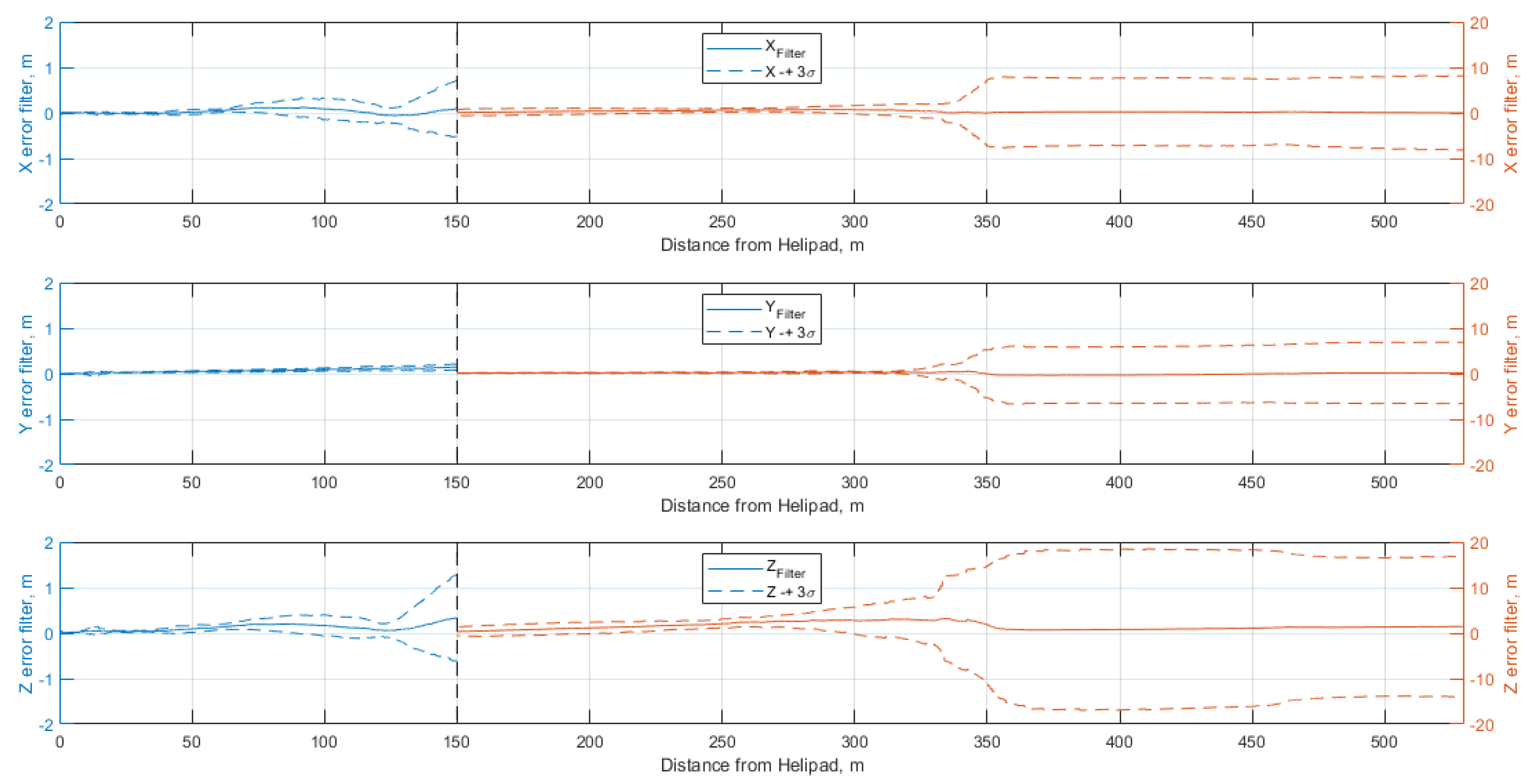
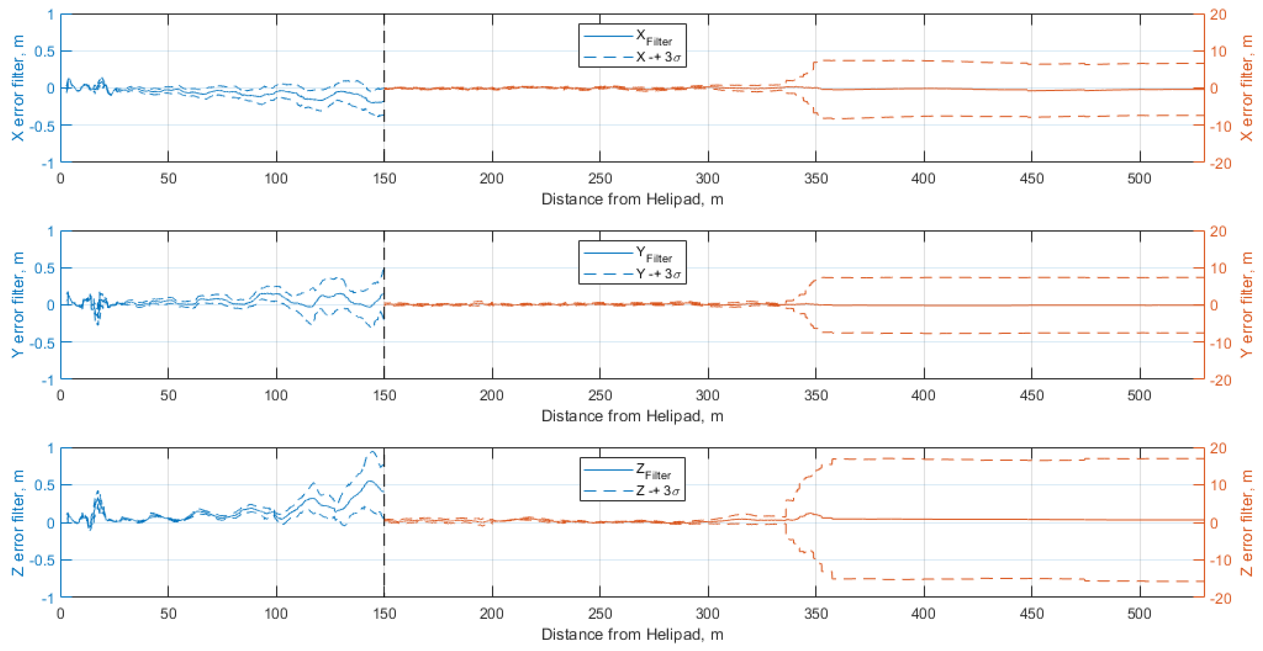
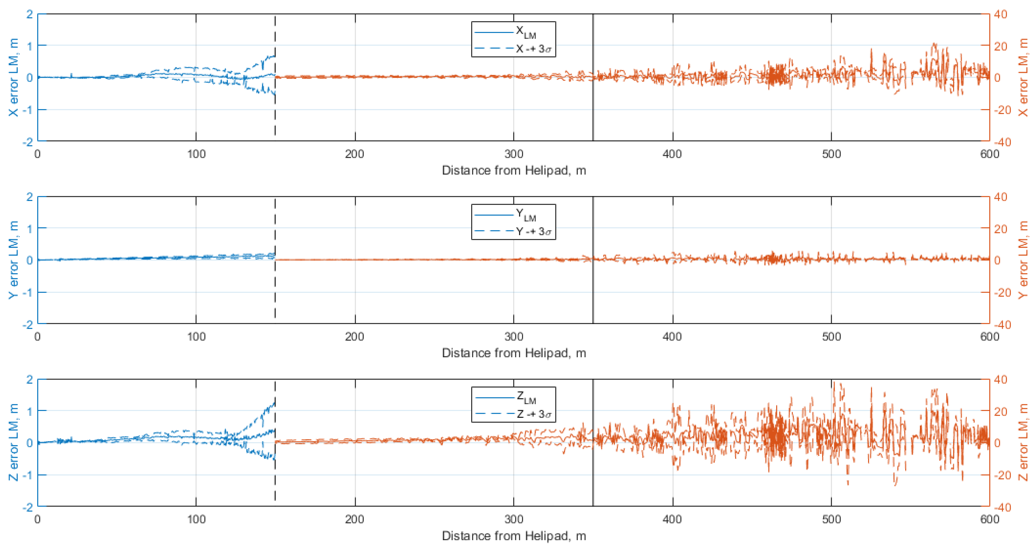
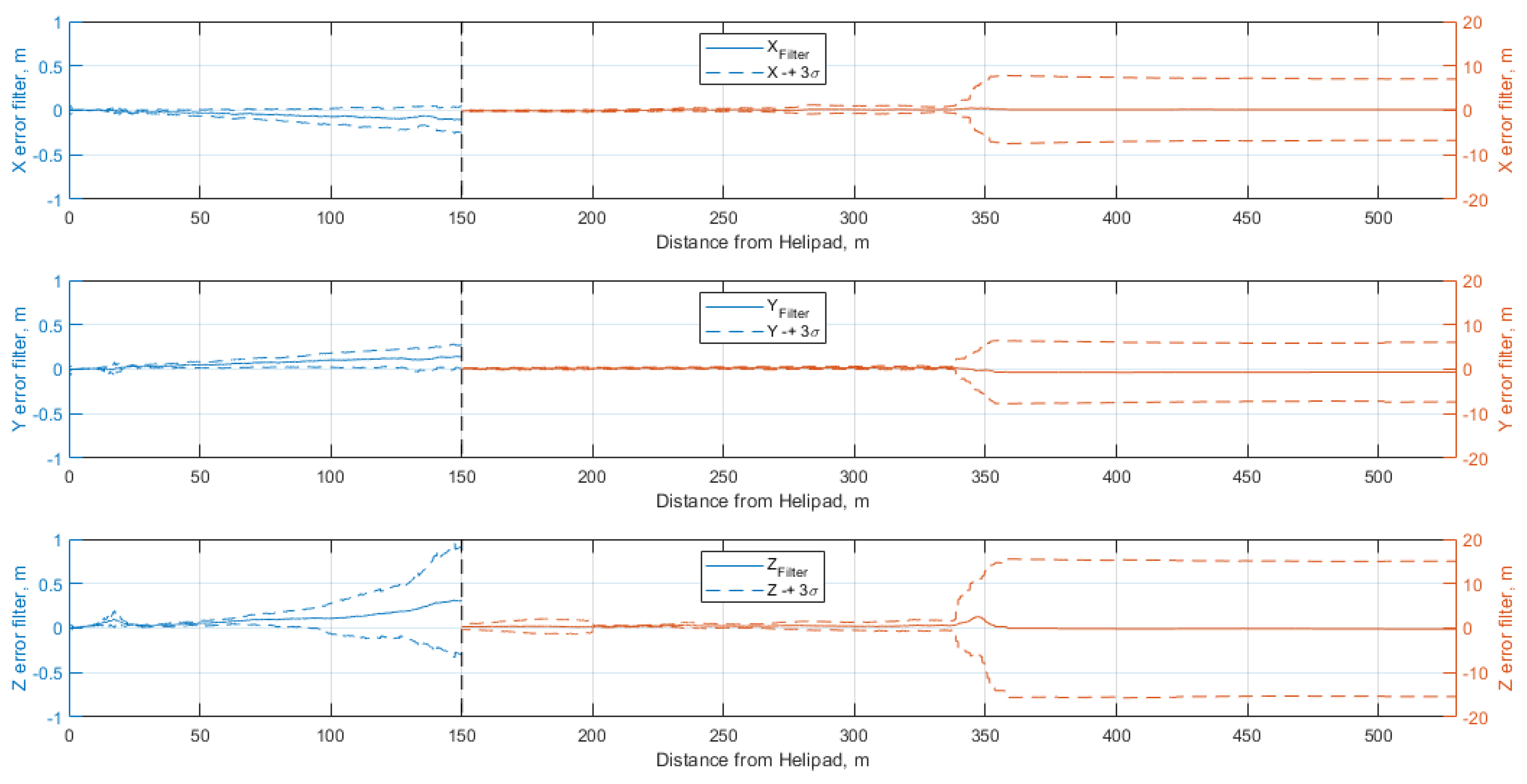
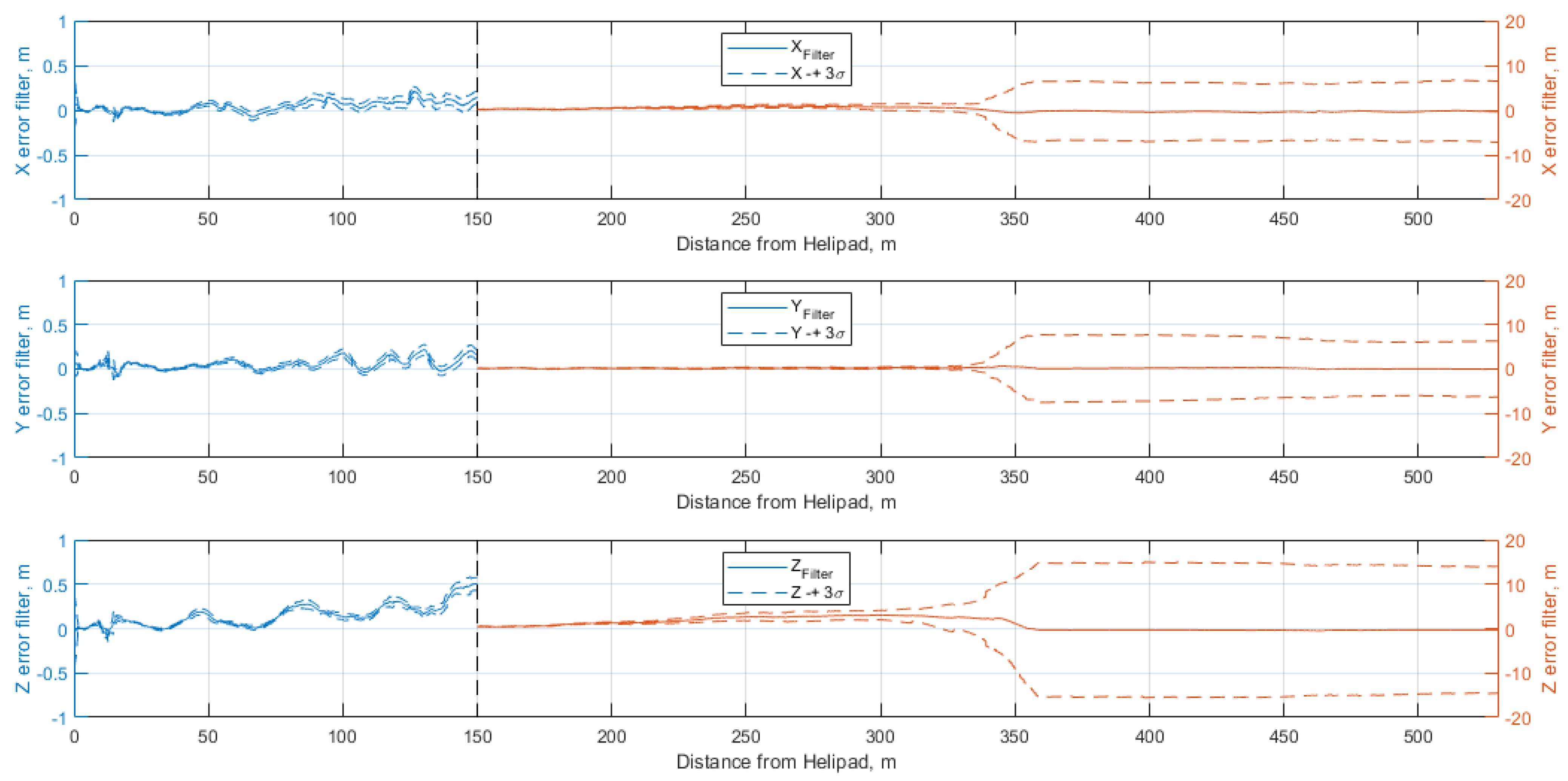
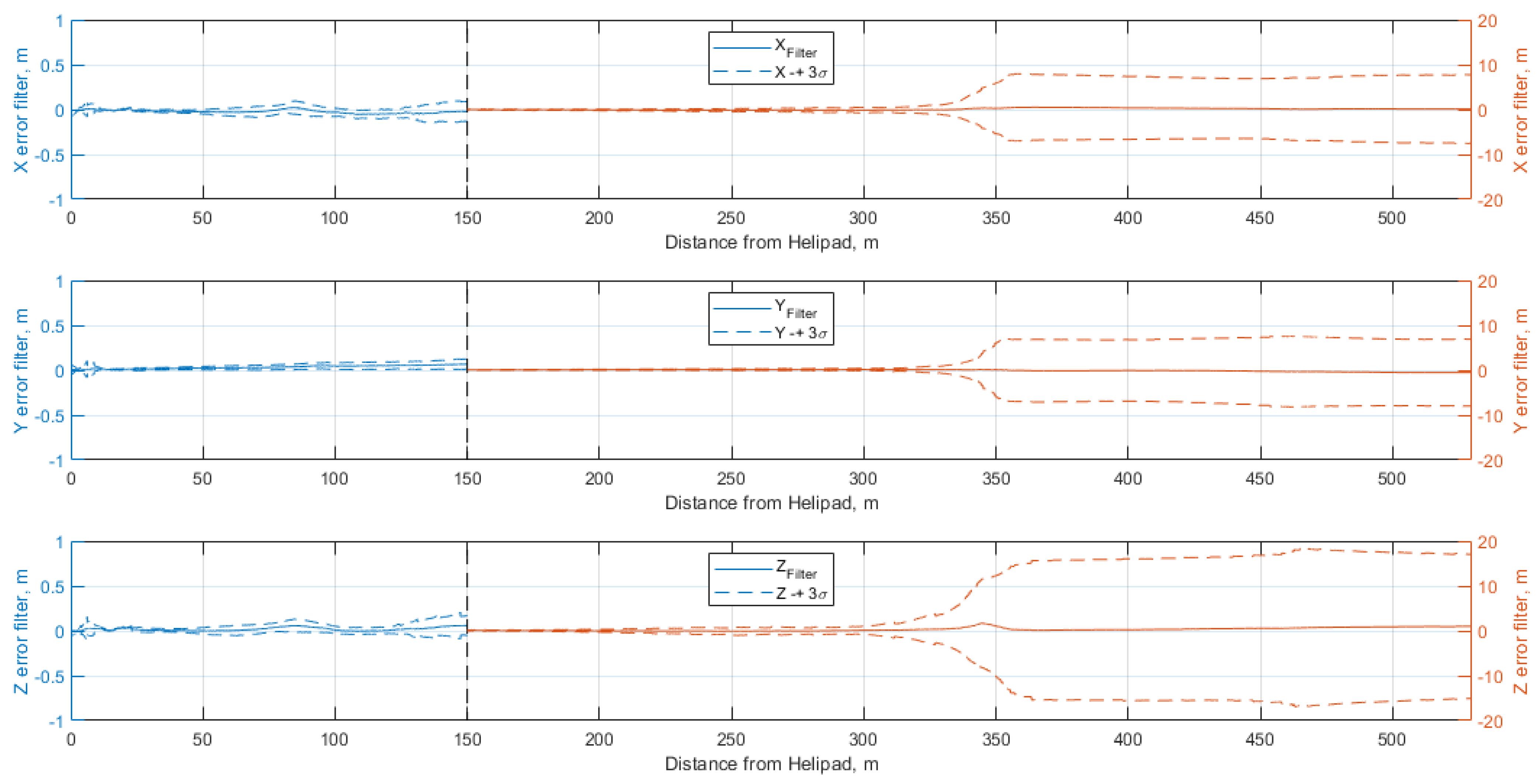
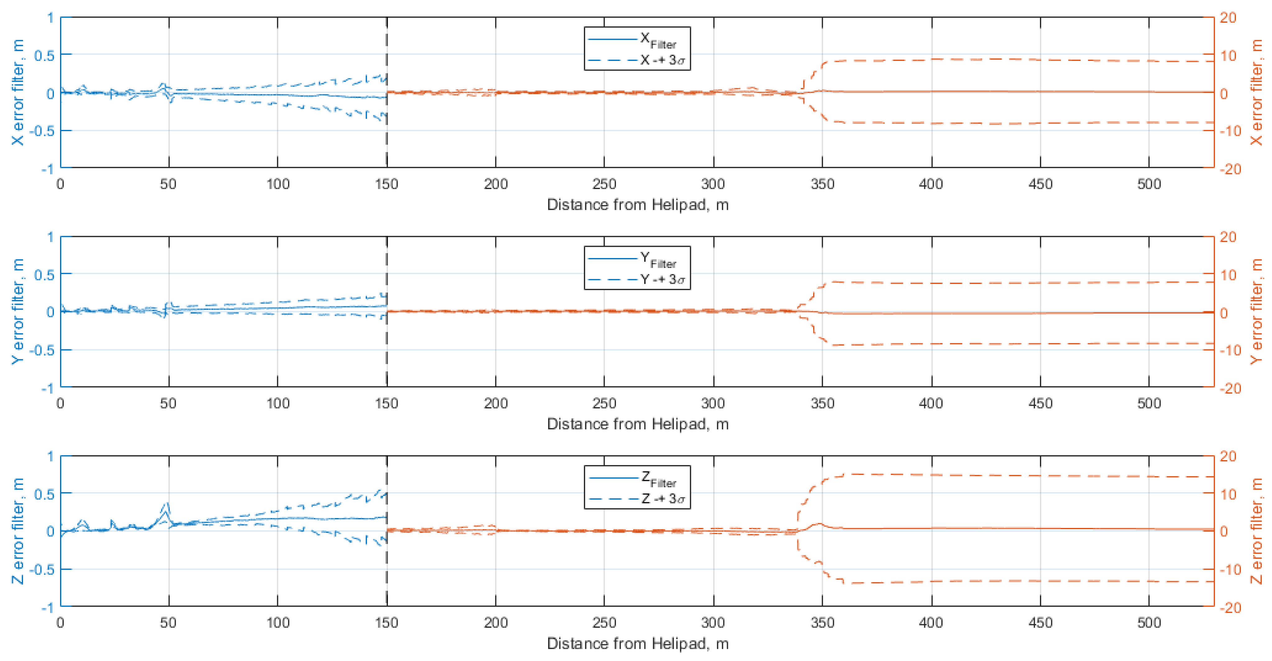
5.2. EKF Performance

The following test cases have been selected to validate the previously introduced filter architecture.

• Daylight: VTCA and 3-stepped trajectories assuming small attitude oscillations of the rotorcraft (maximum 0.1° difference from ideal orientation) to consider its limits in the attitude control capabilities. These scenarios can be used to assess the nominal EKF accuracy.
• Perturbed: VTCA and 3-stepped trajectories assuming larger disturbances applied to the ideal paths (i.e., 0.2 m horizontal displacement and 5° attitude at 1 Hz frequency) to prove the robustness of the vision-aided architecture to significant oscillations caused by atmospheric disturbances.
• Night: VTCA and 3-stepped trajectories in case of night scenario to prove the architecture’s effectiveness in case the pose estimation process relies on the detection of a pattern of lights instead of the AT markers suitable for day-light scenarios.
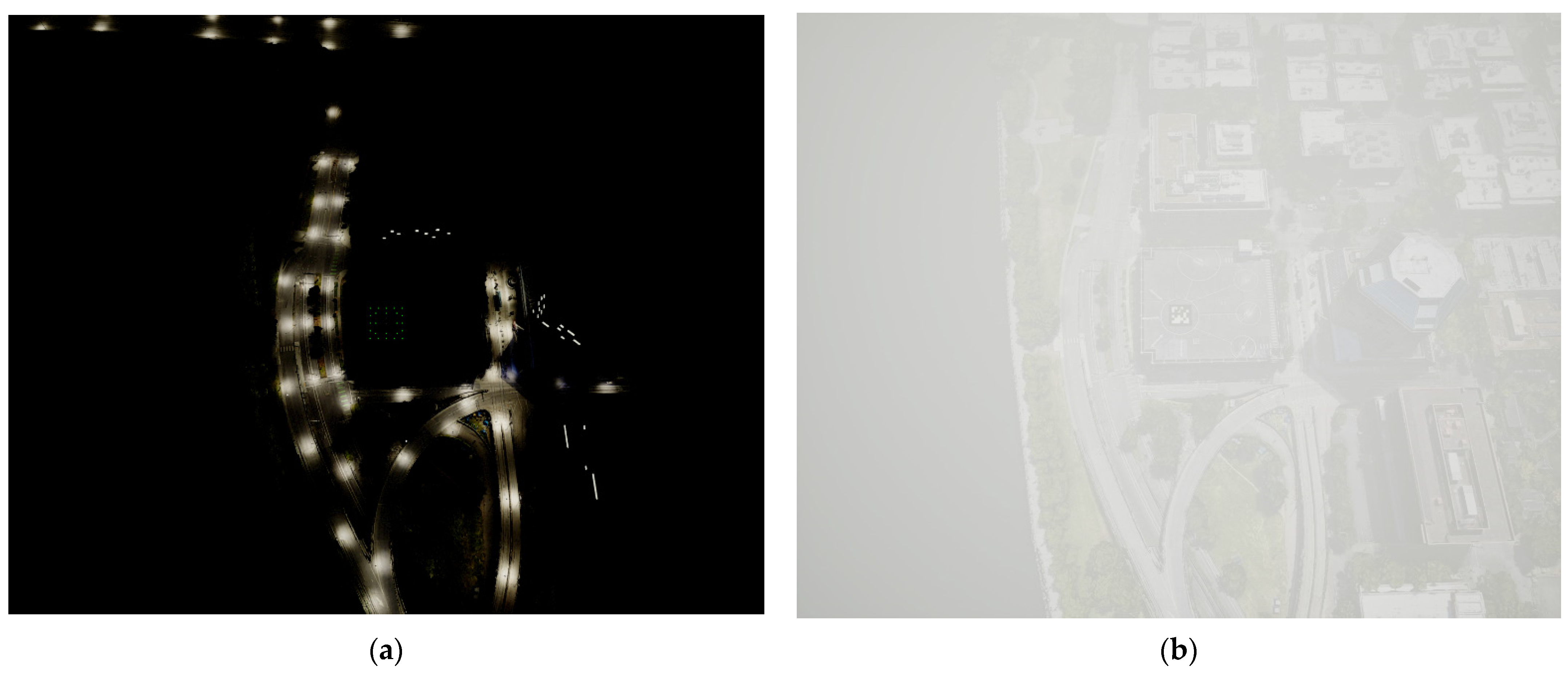
• Low visibility: VTCA trajectory in case of uniform fog to evaluate architecture’s robustness in non-ideal visibility conditions. The AT detections have been reported as a function of the distance from the landing pad, so the same considerations can be applied to the 3-stepped trajectory as well.
• MAP activation: VTCA trajectory in case of local fog banks along the trajectory to test the effective autonomous activation of a MAP.

The trajectory simulated in each test case has a duration of 80 s. In the last three cases, the same disturbance level as in the Daylight case has been considered. Results of each test case are reported through statistical analysis of the filter outputs estimated for multiple repetitions of the selected trajectory to consider the random noise, characterizing IMU and GNSS measurements.

5.2.1. Daylight

Figure 11 and Figure 12 show the EKF positioning error for the VTCA and the 3-stepped landing trajectories, while the positioning error statistics evaluated in different segments of the paths are reported in Table 3 as a function of the reducing distance from the landing pad.

Figure 11. EKF position estimates errors average over 50 simulations and 3−sigma bounds. VTCA landing trajectory in nominal visibility conditions. The plot scale is increased in the last 150 m to better show the errors in the final phase of the approach.

Figure 12. EKF position estimates errors average over 50 simulations and 3−sigma bounds. 3−stepped landing trajectory in nominal visibility conditions. The plot scale is increased in the last 150 m to better show the errors in the final phase of the approach.

Table 3. Mean (μ) and standard deviation (σ) over 50 simulations of the EKF position estimates errors computed along different sections of the trajectories in nominal visibility conditions.

Trajectory	Parameter	550–350 m	350–200 m	200–100 m	100–20 m	20–0 m
VTCA	μx (m)	0.052	0.495	0.096	0.042	0.001
	σx (m)	2.499	0.564	0.214	0.060	0.009
	μy (m)	−0.032	0.257	0.134	0.049	0.007
	σy (m)	2.291	0.376	0.035	0.021	0.011
	μz (m)	1.147	2.291	0.367	0.110	0.026
	σz (m)	5.286	1.551	0.427	0.073	0.022
3-stepped	μx (m)	0.178	0.076	−0.113	−0.037	−0.003
	σx (m)	2.355	0.287	0.069	0.023	0.023
	μy (m)	−0.671	0.239	0.146	0.060	0.009
	σy (m)	2.220	0.218	0.074	0.025	0.030
	μz (m)	−0.095	0.507	0.283	0.069	0.036
	σz (m)	5.030	0.506	0.374	0.036	0.043

The previous plots and the table show that the EKF accuracy in position estimation is dependent on the navigation sensor used in the correction step. The first phase of the approaches, until 350 distance from the landing pad, is influenced by the accuracy of the nominal GNSS receiver selected for the simulations. On the other side, starting from the TPVF, the variance of the filter error gradually decreases until reaching maximum positioning errors of 40 cm in the last 100 m of both the trajectories. The performance is comparable for the two trajectories.

5.2.2. Perturbed

Figure 13 and Figure 14 show the average and 3-sigma bounds computed over 50 simulations of the 2 disturbed trajectories. Table 4 summarizes the statistics of the positioning errors.

Figure 13. EKF position estimates errors average over 50 simulations and 3−sigma bounds. VTCA landing trajectory in nominal visibility conditions with disturbances applied to the path. The plot scale is increased in the last 150 m to better show the errors in the final phase of the approach.

Figure 14. EKF position estimates errors average over 50 simulations and 3−sigma bounds. 3−stepped landing trajectory in nominal visibility conditions with disturbances applied to the path. The plot scale is increased in the last 150 m to better show the errors in the final phase of the approach.

Table 4. Mean (μ) and standard deviation (σ) over 50 simulations of the EKF position estimates errors computed along different sections of the disturbed trajectories in nominal visibility conditions.

Trajectory	Parameter	550–350 m	350–200 m	200–100 m	100–20 m	20–0 m
VTCA	μx (m)	−0.375	0.584	0.160	0.024	0.010
	σx (m)	2.193	0.507	0.101	0.052	0.041
	μy (m)	0.067	0.235	0.116	0.044	0.024
	σy (m)	2.195	0.354	0.081	0.043	0.044
	μz (m)	−0.352	2.371	0.449	0.101	0.025
	σz (m)	4.707	1.022	0.310	0.082	0.059
3-stepped	μx (m)	−0.386	−0.033	−0.137	−0.050	0.001
	σx (m)	2.411	0.300	0.107	0.034	0.064
	μy (m)	−0.110	0.148	0.115	0.046	0.019
	σy (m)	2.452	0.255	0.150	0.044	0.082
	μz (m)	0.816	0.346	0.345	0.081	0.065
	σz (m)	5.246	0.622	0.229	0.050	0.097

The results highlight the robustness of the implemented EKF to trajectory disturbances that might be caused by wind fields in the area around the vertiport. The translation and orientation oscillations of the aircraft are sensed by the IMU, maintaining accurate the results of the EKF prediction step which are used to provide first guesses to the visual pose estimation algorithm. This results in filter positioning errors comparable with the undisturbed trajectories as shown in Table 4. Figure 13 and Figure 14 also confirm that the position estimates are not considerably influenced by the oscillations if compared to the undisturbed case of Figure 11 and Figure 12.

5.2.3. Night

The errors in this scenario are conformal to those achieved in the daylight ones. Figure 15 and Figure 16 show the EKF positioning error for both the VTCA and the 3-stepped landing trajectory, while in Table 5 the positioning error statistics evaluated in different segments of the paths are reported.

Figure 15. EKF position estimates errors average over 50 simulations and 3−sigma bounds. VTCA landing trajectory at night-time. The plot scale is increased in the last 150 m to better show the errors in the final phase of the approach.

Figure 16. EKF position estimates errors average over 50 simulations and 3−sigma bounds. 3−stepped landing trajectory at night-time. The plot scale is increased in the last 150 m to better show the errors in the final phase of the approach.

Table 5. Mean (μ) and standard deviation (σ) over 50 simulations of the EKF position estimates errors computed along different sections of the trajectories at night-time.

Trajectory	Parameter	550–350 m	350–200 m	200–100 m	100–20 m	20–0 m
VTCA	μx (m)	0.235	−0.067	−0.042	−0.015	−0.002
	σx (m)	2.413	0.448	0.034	0.019	0.013
	μy (m)	−0.402	0.126	0.067	0.025	0.009
	σy (m)	2.451	0.358	0.026	0.014	0.012
	μz (m)	0.618	0.160	0.027	0.019	0.015
	σz (m)	5.074	1.073	0.048	0.023	0.019
3-stepped	μx (m)	0.192	−0.083	−0.063	−0.020	−0.005
	σx (m)	2.719	0.261	0.169	0.028	0.018
	μy (m)	−0.436	0.118	0.070	0.029	0.012
	σy (m)	2.658	0.240	0.074	0.022	0.015
	μz (m)	0.668	0.032	0.206	0.109	0.023
	σz (m)	4.599	0.522	0.229	0.052	0.029

The plots and the statistics of the error verify that the different detection technique adopted by the vision algorithm does not affect the accuracy and precision of the EKF position estimates.

5.2.4. Low Visibility

As anticipated before, the EKF architecture has also been tested for low visibility scenarios with the aim to check the robustness of the navigation architecture in challenging visual conditions and prove the autonomous initialization of balked landing procedures in case of failures and anomalies in the landing pad visual tracking algorithm. The first test case introduces a uniform fog in the daylight scenario, reproducing maximum meteorological visibility of 500 m (Figure 17). This parameter represents the distance at which the landing pad is clearly detected by the image processing algorithm (similarly to the Runway Visual Range adopted for the approval of the aircraft’s final approach phase). Consequently, it is not a setting parameter characterizing the creation of the simulation scenario within Unreal Engine, but rather it has been a-posteriori evaluated. Clearly, by modifying the fog parameters (such as density and speed), the maximum meteorological visibility can be indirectly changed.

Figure 17. UE4 reproduction of Portland heliport and its surroundings with uniform fog (reproducing maximum meteorological visibility of 500 m).

In this case, the vision algorithm does not detect the AT marker placed on the landing pad at the initialization of the approach procedure. However, in this case, the postponed marker recognition does not affect the accuracy of the filter position estimates at the transition to the visual flight phase and later in the approach, since the visual algorithm needs few image frames to be correctly initialized and the implemented EKF correction step relies only on GNSS estimates until the selected distance of 350 m. In case of worse meteorological visibility conditions not allowing the markers to be recognized at 350 m distance, the implemented EKF would autonomously impose a MAP when the estimated covariance of the EKF reaches the imposed threshold. The positioning errors in meters are almost identical to the previous cases and are thus not reported. Indeed, it is interesting to analyze the image processing error, i.e., the error in extracting the corners from the images, to verify if and how it is affected by the degraded visibility conditions. This is done in Figure 18, which reports the difference between the positions of the corners recognized by the image processing algorithm and their reprojections estimated through the true markers’ pose in both the daylight (a) and the low-visibility test case (b). The fact that the detection error (i.e., image processing error) has the same order of magnitude in both the cases explains why the resulting positioning errors are similar. Figure 19 reports the difference in the four detected AT corners’ coordinates in the image frames between the nominal visibility case and the introduced low-visibility case.

Figure 18. (a) Daylight: difference between the positions of the corners recognized by the image processing algorithm and their reprojections estimated through the true markers’ pose; (b) Low−visibility: difference between the positions of the corners recognized by the image processing algorithm and their reprojections estimated through the true markers’ pose. Corners’ legend is referred to the biggest marker of Figure 6a.

Figure 19. Difference in pixel coordinates of the 4 detected AT corners between image frames collected in the daylight and in the low−visibility test cases along a VTCA approach trajectory. Corners’ legend is referred to the biggest marker of Figure 6a.

The resulting difference in the AT detections shows that the fog influences the detection accuracy only in the first frames in which the marker is recognized. The low mean and standard deviation of the computed difference confirm that the marker coordinates detected in this case do not considerably affect the following PnP pose estimation process. To confirm that these observations are valid when varying the perturbations applied to the landing trajectory, a VTCA approach with the oscillations introduced in the Perturbed case has been simulated in the same low-visibility scenario (Figure 17). Figure 20 reports the resulting difference of the four detected AT corners’ coordinates in the image frames in the introduced Perturbed case between low-visibility and nominal visibility conditions. Again, the fact that the image processing performance is weakly affected by the degraded visibility conditions justifies that positioning errors also have a similar level in the Perturbed/low visibility test case.

Figure 20. Difference in pixel coordinates of the 4 detected AT corners between image frames collected in the perturbed and in the low−visibility test cases along a VTCA approach trajectory. Corners’ legend is referred to the biggest marker of Figure 6a.

5.2.5. MAP Activation

The MAP activation case tests the effect on the vision-aided filter architecture of the introduction of local fog banks, fully occulting the landing pad, within the previous uniform fog (Figure 21).

Figure 21. UE4 reproduction of Portland heliport and its surroundings with local fog banks.

In this scenario, failures of the visual detection of the AT fiducial markers occur during the approach phase. This induces an increase of the EKF estimated covariance. The approach procedure is effectively interrupted when the positioning uncertainty estimated, as explained in Section 3, reaches the imposed threshold, which linearly decreases from 10 m at the TPVF and 0.2 m in correspondence of the landing pad. Figure 22 shows the defined threshold, the three-dimensional positioning uncertainty as extracted from the EKF covariance matrix, and the effective activation of a MAP after an increase of this value due to the missed detections of the landing pad. When the VTOL reaches a distance of about 184 m, the landing pad in not detected anymore, so that the correction step cannot trust LM-based pose estimate.

Figure 22. Three-dimensional positioning uncertainty as extracted from the EKF covariance matrix in function of the distance from the landing pad in case of VTCA trajectory with a local fog bank which precludes landing pad visibility at 184 m distance from it. The MAP is autonomously initialized at 135 m.

6. Conclusions

In this paper, an analysis of the requirements to adopt vision sensors in UAM vertical landing procedures, and a vision-aided multi-sensor navigation architecture tailored for these scenarios, have been presented. Two vertical landing trajectories defined within the UAM literature have been considered in the study, however the requirements and the vision-aided filter could be adapted to other possible trajectories.

The estimated sensing requirements prove that the currently available vision sensors have a technological level which can support piloted/autonomous vertical landing procedures to vertiports.

As concerns the proposed navigation algorithm, the conducted simulations prove its accuracy and robustness in non-nominal conditions. In fact, remarkable accuracy of position estimates (maximum errors of 40 cm in the last 100 m of the considered trajectories) is provided by the EKF architecture, considering significant disturbances applied to the ideal paths. Furthermore, the same performance has been demonstrated simulating approaches to the same vertiport at night-time, requiring the detection of a pattern of lights instead of the AT fiducial marker adopted for nominal illumination scenes. In non-nominal visibility conditions, the vision algorithm has shown accurate tracking of the AT marker once the landing pad is recognized, maintaining accurate pose estimates in the flight phase relying on visual pose estimates. Otherwise, it has been demonstrated that a MAP procedure can be autonomously initialized if the marker is not detectable in the images and the self-estimated positioning uncertainty exceeds a fixed threshold, e.g., when the UAV flies in a fog bank. Future research will be aimed at enhancing the multi-sensor-based navigation approach, including other sensor technologies, focusing on the ground infrastructure required to better support landing pad detection in complex urban scenarios, and moving towards flight experimentation in controlled scenarios. Furthermore, future activities will tackle the integration of the presented navigation logic with autonomous visual flight guidance and closed-loop control functions.

References

- National Aeronautics and Space Administration. UAM Vision Concept of Operations (ConOps) UAM Maturity Level (UML) 4. 2021. Available online: https://ntrs.nasa.gov/api/citations/20205011091/downloads/UAM%20Vision%20Concept%20of%20Operations%20UML-4%20v1.0.pdf (accessed on 10 January 2022).
- European Union Aviation Safety Agency. Second Publication of Proposed Means of Compliance with the Special Condition VTOL, Doc. No. MOC-2 SC-VTOL. 2021. Available online: https://www.easa.europa.eu/document-library/product-certification-consultations/special-condition-vtol (accessed on 17 January 2022).
- European Union Aviation Safety Agency Vertiports—Prototype Technical Specifications for the Design of VFR Vertiports for Operation with Manned VTOL-Capable Aircraft Certified in the Enhanced Category (PTS-VPT-DSN). 2022. Available online: https://www.easa.europa.eu/downloads/136259/en (accessed on 27 March 2022).
- Federal Aviation Administration AC 150/5390-2C—Heliport Design. 2012. Available online: https://www.faa.gov/documentLibrary/media/Advisory_Circular/150_5390_2c.pdf (accessed on 7 January 2022).
- Federal Aviation Administration. Draft EB 105, Vertiport Design, June XX. 2022. Available online: https://www.faa.gov/airports/engineering/engineering_briefs/drafts/media/eb-105-vertiport-design-industry-draft.pdf (accessed on 15 March 2022).
- Yilmaz, E.; Warren, M.; German, B.J. Energy and Landing Accuracy Considerations for Urban Air Mobility Vertiport Approach Surfaces. In Proceedings of the AIAA Aviation 2019 Forum, Dallas, TX, USA, 17–21 June 2019. [Google Scholar]
- Webber, D.; Zahn, D. FAA and the National Campaign (Powerpoint). Available online: https://nari.arc.nasa.gov/aam-portal/recordings/ (accessed on 20 February 2022).
- Pradeep, P.; Wei, P. Energy-Efficient Arrival with RTA Constraint for Multirotor EVTOL in Urban Air Mobility. J. Aerosp. Inf. Syst. 2019, 16, 263–277. [Google Scholar] [CrossRef]
- Kleinbekman, I.C.; Mitici, M.; Wei, P. Rolling-Horizon Electric Vertical Takeoff and Landing Arrival Scheduling for on-Demand Urban Air Mobility. J. Aerosp. Inf. Syst. 2020, 17, 150–159. [Google Scholar] [CrossRef]
- Shao, Q.; Shao, M.; Lu, Y. Terminal Area Control Rules and EVTOL Adaptive Scheduling Model for Multi-Vertiport System in Urban Air Mobility. Transp. Res. Part C Emerg. Technol. 2021, 132, 103385. [Google Scholar] [CrossRef]
- Song, K.; Yeo, H.; Moon, J.H. Approach Control Concepts and Optimal Vertiport Airspace Design for Urban Air Mobility (UAM) Operation. Int. J. Aeronaut. Space Sci. 2021, 22, 982–994. [Google Scholar] [CrossRef]
- Song, K.; Yeo, H. Development of Optimal Scheduling Strategy and Approach Control Model of Multicopter VTOL Aircraft for Urban Air Mobility (UAM) Operation. Transp. Res. Part C Emerg. Technol. 2021, 128, 103181. [Google Scholar] [CrossRef]
- Patruno, C.; Nitti, M.; Petitti, A.; Stella, E.; D’Orazio, T. A Vision-Based Approach for Unmanned Aerial Vehicle Landing. J. Intell. Robot. Syst. 2019, 95, 645–664. [Google Scholar] [CrossRef]
- Lin, S.; Jin, L.; Chen, Z. Real-Time Monocular Vision System for UAV Autonomous Landing in Outdoor Low-Illumination Environments. Sensors 2021, 21, 6226. [Google Scholar] [CrossRef] [PubMed]
- Wubben, J.; Fabra, F.; Calafate, C.T.; Krzeszowski, T.; Marquez-Barja, J.M.; Cano, J.C.; Manzoni, P. Accurate Landing of Unmanned Aerial Vehicles Using Ground Pattern Recognition. Electronics 2019, 8, 1532. [Google Scholar] [CrossRef] [Green Version]
- Chen, X.; Phang, S.K.; Chen, B.M. System Integration of a Vision-Guided UAV for Autonomous Tracking on Moving Platform in Low Illumination Condition. In Proceedings of the Institute of Navigation Pacific Positioning, Navigation and Timing Meeting, Honolulu, HI, USA, 1–4 May 2017; pp. 1082–1092. [Google Scholar]
- Chen, X.; Lin, F.; Hamid, M.R.A.; Teo, S.H.; Phang, S.K. Real-Time Landing Spot Detection and Pose Estimation on Thermal Images Using Convolutional Neural Networks. In Proceedings of the 2018 IEEE 14th International Conference on Control and Automation (ICCA), Anchorage, AL, USA, 12–15 June 2018; pp. 998–1003. [Google Scholar]
- Baldini, F.; Anandkumar, A.; Murray, R.M. Learning Pose Estimation for UAV Autonomous Navigation and Landing Using Visual-Inertial Sensor Data. In Proceedings of the 2020 American Control Conference (ACC), Denver, CO, USA, 1–3 July 2020; pp. 2961–2966. [Google Scholar]
- Ye, S.; Wan, Z.; Zeng, L.; Li, C.; Zhang, Y. A Vision-Based Navigation Method for EVTOL Final Approach in Urban Air Mobility (UAM). In Proceedings of the 2020 4th CAA International Conference on Vehicular Control and Intelligence (CVCI), Hangzhou, China, 18–20 December 2020; pp. 645–649. [Google Scholar]
- Kawamura, E.; Kannan, K.; Lombaerts, T.; Ippolito, C.A. Vision-Based Precision Approach and Landing for Advanced Air Mobility. In Proceedings of the AIAA SCITECH 2022 Forum, Reston, VA, USA, 3 January 2022. [Google Scholar]
- EUROCONTROL. Helicopter Point in Space Operations in Controlled and Uncontrolled Airspace Generic Safety Case. Edition Number 1.4. 2019. Available online: https://www.eurocontrol.int/publication/helicopter-point-space-operations-controlled-and-uncontrolled-airspace (accessed on 15 February 2022).
- Vascik, P.D.; Hansman, R.J. Development of Vertiport Capacity Envelopes and Analysis of Their Sensitivity to Topological and Operational Factors. In Proceedings of the AIAA Scitech 2019 Forum, AIAA, San Diego, CA, USA, 7–11 January 2019. [Google Scholar]
- EVTOL Aircraft Directory. Available online: https://evtol.news/aircraft (accessed on 31 March 2022).
- Bauranov, A.; Rakas, J. Designing Airspace for Urban Air Mobility: A Review of Concepts and Approaches. Prog. Aerosp. Sci. 2021, 125, 100726. [Google Scholar] [CrossRef]
- Galway, D.; Etele, J.; Fusina, G. Modeling of Urban Wind Field Effects on Unmanned Rotorcraft Flight. J. Aircr. 2011, 48, 1613–1620. [Google Scholar] [CrossRef]
- Zelinski, S. Operational Analysis of Vertiport Surface Topology. In Proceedings of the AIAA/IEEE Digital Avionics Systems Conference, San Antonio, TX, USA, 11–15 October 2020; pp. 1–10. [Google Scholar]
- Federal Aviation Administration AC 20-167A. Airworthiness Approval of Enhanced Vision System, Synthetic Vision System, Combined Vision System, and Enhanced Flight Vision System Equipment. 2016. Available online: https://www.faa.gov/documentLibrary/media/Advisory_Circular/AC_20-167A.pdf (accessed on 7 January 2022).
- Shelton, K.J.; Williams, S.P.; Kramer, L.J.; Arthur, J.J.; Prinzel, L., II; Bailey, R.E. External Vision Systems (XVS) Proof-of-Concept Flight Test Evaluation. In Proceedings of the SPIE Defense and Security Symposium, Baltimore, MD, USA, 19 June 2014; Volume 9087. [Google Scholar]
- Link, N.K.; Kruk, R.; McKay, D.; Jennings, S.A.; Craig, G. Hybrid Enhanced and Synthetic Vision System Architecture for Rotorcraft Operations. In Proceedings of the SPIE AeroSense, Orlando, FL, USA, 16 July 2002; Volume 4713. [Google Scholar]
- Groves, P. Principles of GNSS, Inertial, and Multisensor Integrated Navigation Systems, 2nd ed.; Artech: Morristown, NJ, USA, 2013. [Google Scholar]
- Bijjahalli, S.; Sabatini, R.; Gardi, A. GNSS Performance Modelling and Augmentation for Urban Air Mobility. Sensors 2019, 19, 4209. [Google Scholar] [CrossRef] [PubMed] [Green Version]
- Maia, F.D.; Lourenço da Saúde, J.M. The State of the Art and Operational Scenarios for Urban Air Mobility with Unmanned Aircraft. Aeronaut. J. 2021, 125, 1034–1063. [Google Scholar] [CrossRef]
- Olson, E. AprilTag: A Robust and Flexible Visual Fiducial System. In Proceedings of the 2011 IEEE International Conference on Robotics and Automation, Shanghai, China, 9–13 May 2011; pp. 3400–3407. [Google Scholar]
- Blackman, S.S.; Popoli, R. Design and Analysis of Modern Tracking Systems; Artech House: London, UK, 1999. [Google Scholar]
- Gavin, H.P. The Levenberg-Marquardt Algorithm for Nonlinear Least Squares Curve-Fitting Problems; Duke University: Durham, NC, USA, 2020. [Google Scholar]
- Szeliski, R. Computer Vision—Algorithms and Applications; Springer: London, UK, 2011. [Google Scholar]